Abstract
Exploring the mechanisms that drive land use and cover change (LUCC) is essential for informing the formulation and implementation of effective policies aimed at optimizing land use patterns. In this study, we examined the spatial and temporal patterns of LUCC within the Lancang–Mekong River Basin (LMRB) using Globeland30 data for the years 2000, 2010, and 2020. Firstly, we analyzed the quantitative characteristics of LUCC within the LMRB in terms of the value of change and rate of change. Additionally, we investigated the converting characteristics of LUCC within the LMRB by employing land use transition matrices and land use transition probability matrices. Furthermore, we depicted the spatial distribution of LUCC within the LMRB through land use mapping and statistical analysis. The results indicate a substantial decline in forests, coupled with a notable expansion in cultivated land. Given the vital role of forests as carbon sinks, reforestation can enhance ecological services and address challenges related to climate change. Converting cultivated land to forests is an effective human intervention promoting forest transition. This study applies binary logistic models to explore the mechanisms that influence the conversion from cultivated land to forests. The results reveal that slopes ranging from 5° to 15° have the lowest probability of conversion, whereas distances between the cultivated land and the nearest tourist attraction ranging from 9 km to 18 km have the highest probability. Moreover, the conversion process is positively associated with traffic conditions and significantly influenced by human interventions. Within the study area, China, Laos, and Myanmar show a tendency to convert cultivated land into natural LULC types, while Cambodia, Thailand, and Vietnam tend to encroach on cultivated land and expand artificial surfaces. Promoting ecological restoration in the LMRB requires cooperation among these countries.
1. Introduction
Land use and cover change (LUCC) was launched in 1994 as a Core Project of the International Geosphere-Biosphere Programme (IGBP). With the global population continuously growing, urbanization accelerating, and economic development advancing, formulating land use policies that promote the rational use of land resources and mitigate the negative ecological impacts of LUCC, such as soil erosion [1], water resource scarcity [2], biodiversity loss, and other ecological damage, while addressing the negative effects of urban expansion and urban–rural disparity to realize a balance between economic development, ecological protection, and social equity, has become a crucial focus for academics in interdisciplinary fields [3]. Land change science (LCS) is a disciplinary field that focuses on studying LUCC. Analyzing LUCC can guide the preparation of territorial planning, protect the ecological environment, and optimize the patterns of LUCC, which can promote sustainable development in LUCC. Research in this area encompasses diverse topics, including ecosystem services [4], remote sensing monitoring [5], optimization of land use and land cover (LULC) [6], policy impacts [7], climate change [8], efficiency of land use, and biodiversity conservation. In recent years, the analysis of LUCC has made significant progress in data acquisition and processing, method innovation and integration, and exploration of factors influencing LUCC. Notably, technological advancements have greatly enhanced the ability to acquire and process data related to LULC [9]. For example, tools like the Google Earth Engine [10] and cloud computing platforms have revolutionized spatial information acquisition for LUCC analysis. Remote sensing technology enables large-scale and high-resolution data collection, while GIS facilitates LULC classification, intensity calculation, and spatial pattern analysis. The application of machine learning algorithms [11], incorporation of landscape ecology indicators for LULC pattern evaluation [12], and integration of remote sensing, GIS, and model simulation techniques [13] represent notable innovations in LCS. Additionally, various models have been employed to explore the driving factors behind LUCC, including system dynamics model [14], multi-factor driving model [1,15], and predictive models, such as the cellular automata model [16] and Bayesian hierarchical spatiotemporal models [17], among others.
Relevant studies have pointed out that Southeast Asia has been experiencing large-scale forest loss in recent years [13,18,19]. The Food and Agriculture Organization (FAO) [20] points out the vital role of forests. The loss of the protective function provided by forests, such as shading the soil surface and stabilizing soil and rocks, can lead to problems like landslides, soil erosion, and declining water quality. These environmental degradations can have serious consequences for both the ecosystem and human communities in the affected areas [21]. To increase forest cover, two approaches can be considered: firstly, establishing a protected area for forests more likely converted into other LULC types; secondly, converting other LULC types into forests can actively contribute to increasing forest cover. The conversion of other LULC types to forests can significantly enhance the ecological services of land, amplify carbon sequestration and storage capacities, and contribute to a reduction in greenhouse gas emissions. The driving force of LUCC varies greatly with space, time, and land use type [18]. The Lancang–Mekong River Basin (LMRB), encompassing the largest watershed in Southeast Asia, contains a diverse range of LULC types, as well as significant variations in topography and geomorphology. Yun et al. [22] predicted an increasing probability of simultaneous wetting in both upstream and downstream areas within the LMRB, accompanied by a decreasing likelihood of wet/dry differences between these regions. Consequently, the potential for upstream and downstream competition for water resources is expected to rise among the countries within the LMRB.
The objective of this paper is to investigate the extent of deforestation within the LMRB during the period of 2000–2020 by analyzing the spatio-temporal patterns of LUCC. Additionally, we aim to find out how to increase forest cover within the LMRB. To achieve this, we examined the spatial and temporal patterns of LUCC within the Lancang–Mekong River Basin (LMRB) using the Globeland30 data for the years 2000, 2010, and 2020. The findings of our study reveal that the extent and rate of forests degraded in the second decade (2010–2020) were larger than those in the first decade (2000–2010). The most important destination for deforestation within the LMRB is cultivated land, which holds the largest share of non-forest land cover within the basin. Previous research suggests a U-shaped curve relationship between changes in forested land area and regional economic and social development [14]. This trend is closely associated with changes in cultivated land. Instead of resorting to forest logging, it is advisable for the government to promote measures aimed at improving the quality of cultivated land from a soil science perspective. Enhancing the quality of cultivated land can increase agricultural productivity to meet the food demands of the region. A theoretical framework was established to explore the factors influencing land conversion [23]. In this study, we explore the mechanisms driving the conversion from cultivated land to forests using logistic regression. And we assume that the conversion of cultivated land to forests is influenced by three aspects. Firstly, natural factors include elevation and slope. Secondly, locational factors include distance to the nearest main road, distance to the nearest tourist attraction, and distance to the nearest town center. Lastly, socio-economic factors include changes in population density and changes in nighttime light. Population density is highly correlated with agricultural activities, and nighttime light is highly correlated with industrial production. The overlap of these factors can reflect the socio-economic level of the area to some extent, including formal and informal economic activities [24]. In summary, by studying the spatio-temporal patterns of LUCC and understanding the mechanisms that drive the conversion of cultivated land into forests can develop strategies to increase forest cover and improve land management practices in critical regions such as the LMRB.
2. Materials and Methods
2.1. Study Area
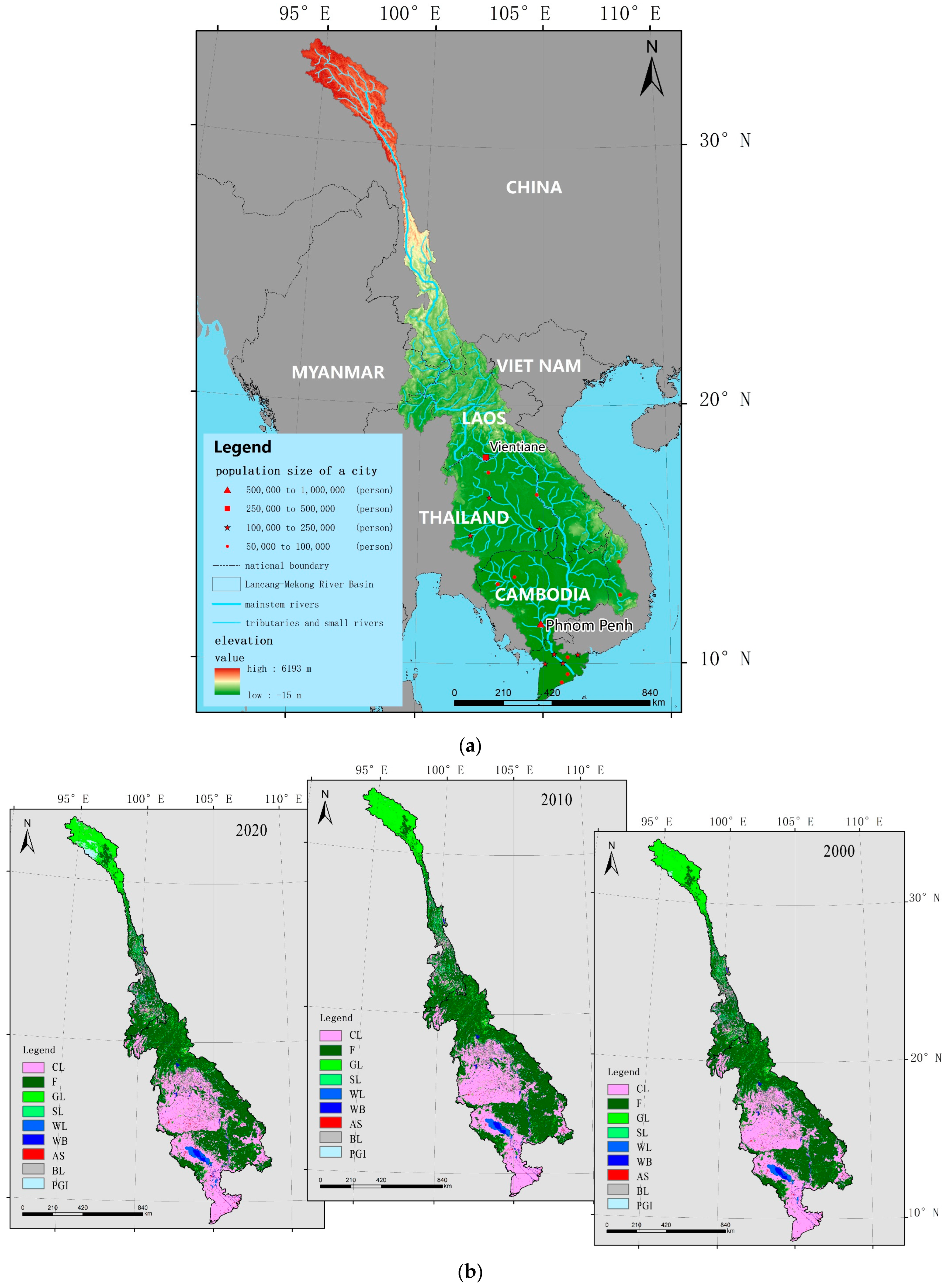
The Lancang–Mekong River is a significant transboundary river in Asia, spanning a total length of 4880 km and flowing through six countries: China, Laos, Myanmar, Thailand, Cambodia, and Vietnam (Figure 1). It ultimately discharges into the South China Sea south of Ho Chi Minh City in Vietnam. The river system contains mainstem rivers, tributaries, and small rivers. The delineation of the water system within the study area is based on research conducted by Wang and their team [25]. According to a study by Munia et al. [26], the upstream area of the LMRB is identified as the watershed located in China and Myanmar. On the other hand, the downstream area encompasses watersheds situated in Thailand, Laos, Vietnam, and Cambodia. The LMRB covers a vast area within a range from 8.4° N to 33.9° N and 93.7° E to 109.5° E, with a total basin area of approximately 81,810,571.14 hectares. When it comes to land distribution, Laos accounts for about 25.65% of the basin area, followed by Thailand (23.36%), China (20.90%), Cambodia (19.23%), Vietnam (8.10%), and Myanmar (2.76%). The terrain within the basin is characterized by highlands in the northwest and lowlands in the southeast, with elevations ranging from −15 m to 6193 m. LULC types in the upstream area are predominantly composed of permanent glaciers and ices, grasslands, and forests. In contrast, the downstream area is dominated by forests, cultivated land, water bodies, wetlands, and a relatively larger extent of artificial surfaces. Within the study area, there is one city with a population exceeding 500,000, namely Phnom Penh, and one city with a population ranging from 250,000 to 500,000, namely Vientiane. Additionally, there are seven cities with populations ranging from 100,000 to 250,000, including Khon Kaen, Nakhon Ratchasima, Ubon Ratchathani, Can Tho, My Tho, Rach Gia, and Long Xuyen. Moreover, there are at least 47 other cities within the LMRB with populations less than 100,000 people.

Figure 1.
(a) Map of the study area; (b) land use map across the study area. CL means cultivated land, F means forest, GL means grassland, SL means shrubland, WL means wetland, WB means water body, AS means artificial surface, BL means bare land, PSI means permanent snow and ice.
2.2. Data Source and Introduction
Various LULC datasets exist. In comparison to the ESA Land Cover CCI dataset and the land use data provided by Copernicus European Earth monitoring program (Global Land Service (GIO-GL)), which were co-recommended by Mora et al. [27] for monitoring progress towards Sustainable Development Goals, the Globeland30 data developed by National Geomatics Center of China (NGCC) include ten LULC types at a spatial resolution of up to 30 m [28,29]. This LULC product was derived from a pixel-object-knowledge (POK)-based operational mapping approach, utilizing over 20,000 Landsat and Chinese HJ-1 satellite images. The overall classification accuracy achieved was over 80% after careful processing and analysis [30]. To acquire the explanatory variables, data from various platforms were utilized. First, we got digital elevation model (DEM) data with 30 m spatial resolution were obtained from the United States Geological Survey. As for the slope data, we produced them from DEM data. Then, we obtained town centers, main roads, and tourist sites from OpenStreetMap. Finally, the population density data were from the Oak Ridge National Laboratory. Additionally, Professor Yu’s team overcame the difficulty of the non-comparison between DMSP-OLS data and NPP-VIIRS data [31] and provided nighttime light data for the years 2000, 2010, and 2020.
2.3. Method of Analysis and Data Processing
2.3.1. Land Use Transition Matrix and Land Use Transition Probability Matrix
The land use transition matrix is a cross-tabulation matrix used to compare two maps from different points in time, allowing for the assessment of total change in land categories. It consists of four components: net change, swap, gross gains, and gross losses [32]. Net change provides valuable information about definite changes in the landscape, but it is crucial to recognize that the absence of net change does not necessarily indicate a lack of change. The swap component of change, where categories change location while maintaining the same quantity, should also be considered when analyzing landscape changes. However, the diverse range of LULC types present in the study area makes it comparatively complex for the land use transition matrix to reflect the characteristics of LUCC. To improve the readability of the matrix, two steps are followed to convert the land use transition matrix (T) into a land use transition probability matrix (P). represents the number of transitions from land use category i to category j. First, for each row in the transition matrix, the sum of all values in that row is calculated to obtain the total transition quantity for each land use category. Second, each element in the transition matrix is divided by its corresponding total transition quantity obtained in the previous step. This transformation yields the land use transition probabilities, which represent the likelihood of transitioning from one land use category to another.
2.3.2. Logistic Regression
Logistic regression is a commonly used statistical method for analyzing factors that influence dichotomous or multi-categorical problems. In a study by Sun et al. [33], they employed single-factor logistic regression analysis, multi-factor logistic regression analysis, and stratified logistic regression analysis to analyze the driving factors. Binary logistic regression is a statistical method used to predict the outcome of a dichotomous dependent variable based on previous observations. In the study, a binary logistic regression model was applied to explore the effect of explanatory variables on response variable, as expressed in Formula (1). In the formula, P indicates the probability of an event occurring, while 1 − P indicates the probability of the event not occurring. X means the set of explanatory variables in the study, including , and means the set of regression coefficients to be determined, including .
In single-factor logistic regression analysis, variables with an asymptotic significance level greater than 0.05 are excluded from the range of driving factors explored in the next step [34]. In multi-factor logistic regression analysis, researchers often evaluate the performance of the logistic regression model by examining the area under the receiver operating characteristic curve (AUC). Fawcett [35] introduced receiver operating characteristic (ROC) analysis in 2006, highlighting that ROC graphs can provide a more comprehensive measure of classification performance compared to scalar measures, such as overall accuracy (OA), error rate, or error cost. To optimize the model for higher AUC or OA, some researchers exclude variables with poor independence. To investigate the impact of each factor on the conversion from cultivated land to forests, factors in the model were discretized, and reference categories were selected.
2.3.3. Data Processing
This section contains two parts. First, we analyze the spatio-temporal patterns of LUCC in the LMRB during 2000–2020 through constructing land use transition matrices and land use transition probability matrices. This analysis is conducted using the raster calculator function in GIS software (ArcMap 10.7) and the pivot table function in Excel. The LMRB-wide land use transition matrices and land use transition probability matrices are calculated based on the Globeland30 data for the years 2000, 2010, and 2020.
Second, in terms of acquiring the response variable and the explanatory variables for analyzing the impact mechanism of the conversion from cultivated land to forests, the data processing involved several steps. To acquire response variable, with the help of GIS software (ArcMap 10.7 and ArcGIS pro 10.3), following steps were carried out: (1) the Spatial Analyst Tool named Raster Calculator was applied to define the attribute value of the spatial unit that changed within the study area as 1 and the attribute value of the spatial unit that did not change as 0; (2) within the spatial range of the spatial unit with an attribute value of 1, the Spatial Analyst Tool named Extract by Attributes was applied to obtain the raster data of cultivated land change to other LULC types; (3) the Conversion Tool named From Raster to Polygon was applied to convert the raster data into vector data; (4) random point data were created within the spatial extent constrained by the vector data; (5) the Spatial Analyst Tool named Extract Multi-values to Points was applied to assign land use type attributes to the random point data in the initial and final years, where the attribute for conversion of land use type from cultivated land to forests is defined as 1 and the attribute for conversion of land use type from cultivated land to other LULC types is defined as 0. To acquire explanatory variables (see more in Table 1), with the help of the GIS software (ArcMap 10.7 and ArcGIS pro 10.3), following steps were carried out: (1) the Spatial Analysis Tool called Slope Analysis Tool was used to generate slope data at 30 m resolution based on the DEM data; (2) the Spatial Analyst Tool called Euclidean Distance was used to generate data, including the distance to the nearest main road, the distance to the nearest tourist attraction, and the distance to the nearest town center; (3) another Spatial Analyst Tool named Raster Calculator was used to generate data, including the change in population density and nighttime light; (4) the values of the explanatory variables were assigned to the attribute table of the random point data with the help of the Spatial Analyst Tool named Extract Multi-values to Points.

Table 1.
Explanatory variables involved in exploring mechanisms impacting LUCC.
It is worth mentioning that certain measures were taken to address spatial autocorrelation and potential bias in the analysis. To mitigate the effect of spatial autocorrelation, the minimum distance between points was set to be no less than 50 m. Additionally, to reduce bias, efforts were made to maintain a balanced ratio of sample points between the two classes (0 and 1), aiming for a close to 1:1 ratio. This ensured that the samples were representative. In summary, the attribute tables of the random point data containing the Y (response variable) and X (explanatory variables) values were exported and saved as Excel files. The entire workflow of the study is depicted in Figure 2.
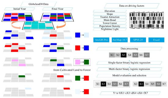
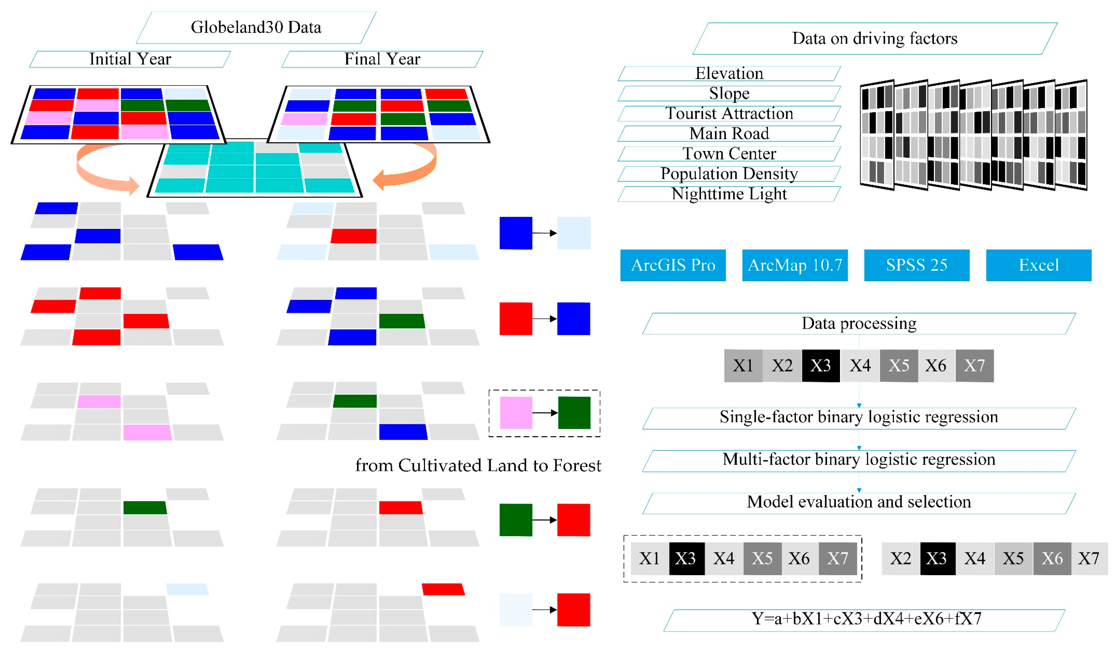
Figure 2.
Flowchart of this study.
3. Results
3.1. Characteristics of the LULC in the LMRB
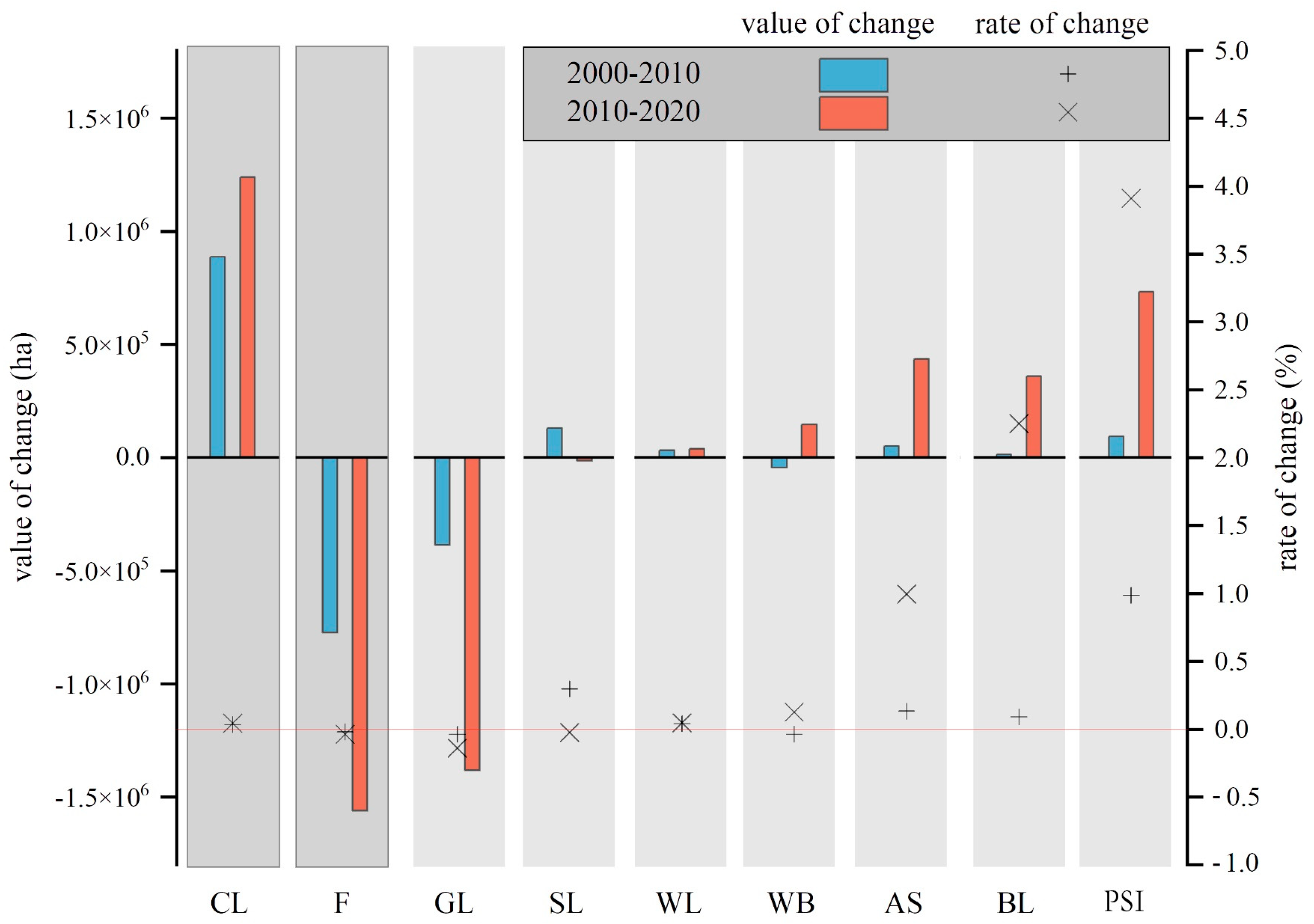
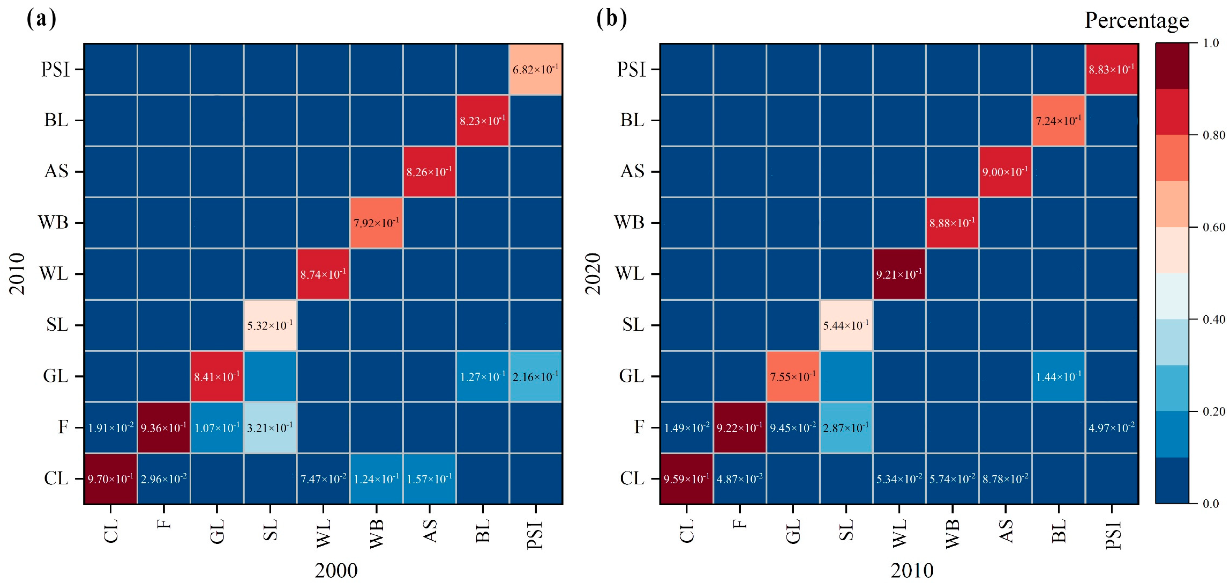
This section analyses the quantitative characteristics of a single LULC type and the converting characteristics between each two LULC types within the LMRB based on the Globeland30 data. On the one hand, when it comes to the quantitative characteristics of a single LULC type, this study portrayed it in terms of the quantitative structure, value of change, and rate of change. Firstly, forests and cultivated land were the two types with the highest proportions of all LULC types in these three years within the LMRB (Table 2). Secondly, forests and cultivated land were the two main LULC types that changed in the two decades within the LMRB (Figure 3). Finally, compared to the period from 2000 to 2010, the LULC types except for shrublands underwent relatively greater changes from 2010 to 2020 within the LMRB (Figure 3). On the other hand, when it comes to the converting characteristics between each two LULC types within the LMRB, this study portrayed it with the help of the land use transition matrices and land use transition probability matrices (Table 3 and Table 4, and Figure 4). Firstly, over the past two decades, more than 50% of the area of all LULC types have remained unchanged. Among all LULC types, cultivated land and forests are the two most stable LULC types, while shrublands is the least stable. Secondly, conversions from forests to cultivated land and grasslands and conversions from cultivated land and grasslands to forests are the four main conversions ranked as the top five in terms of area. Additionally, in the second decade, the conversion from grasslands to permanent snows and ices replaced the conversion from grasslands to cultivated land as one of the main conversions ranked as the top five in terms of area. Finally, cultivated land has been converted more to artificial surfaces than to grasslands, except for conversion from cultivated land to forests. Grasslands have been converted more to permanent snows and ices than to cultivated land, except for conversion from grasslands to forests. Bare lands have been converted more to permanent snows and ices than to forests, except for conversion from bare lands to grasslands.
Table 2.
Proportion of the area of each LULC type in the LMRB by year.

Figure 3.
Value of change and rate of change in area for each LULC type in each decade from 2000 to 2020 within the LMRB. CL means cultivated land, F means forest, GL means grassland, SL means shrubland, WL means wetland, WB means water body, AS means artificial surface, BL means bare land, PSI means permanent snow and ice.
Table 3.
Land use transition matrix within the LMRB during 2000–2010.
Table 4.
Land use transition matrix within the LMRB during 2010–2020.
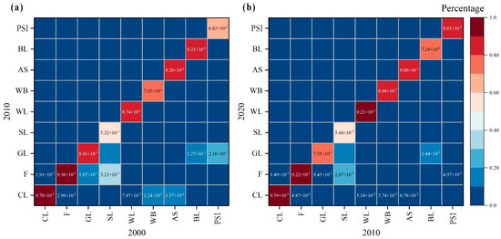
Figure 4.
Land use transition probability matrix within the LMRB during: (a) 2000–2010; (b) 2010–2020. CL means cultivated land, F means forest, GL means grassland, SL means shrubland, WL means wetland, WB means water body, AS means artificial surface, BL means bare land, PSI means permanent snow and ice.
3.2. Regional Differentiation Pattern in the LMRB
This section focuses on analyzing the divergence pattern in the quantity and transfer of each LULC type in each country within the LMRB using the Globeland30 data for the years 2000, 2010, and 2020. The study area was divided into six spatial units by the national administrative boundary. To analyze the differentiation pattern in LULC, net change and gain/loss change for each LULC type were examined. The net change provides an overall perspective on LUCC, while the gain/loss change focuses on specific aspects to identify areas of increases and decreases.
On a practical level, Cambodia emerged as the main contributor to the net change in cultivated land within the LMRB over the two decades analyzed. Cambodia surpassed Laos as the primary contributor to the increase in cultivated land, while Thailand replaced China as the main contributor to the decrease in cultivated land from 2010 to 2020 compared to the period from 2000 to 2010. Regarding forests, Cambodia replaced Laos as the primary contributing country to the net change in the LMRB from 2010 to 2020 compared to the period from 2000 to 2010. China played a significant role in forest increase, whereas Cambodia replaced Laos as the primary contributor to forest decrease. For more detailed information, refer to Figure 5. To visualize the spatial changes in land use and land cover within the study area from 2000 to 2020, we created a visualization depicting the gains and losses of each LULC type. For more details, refer to Figure 6.
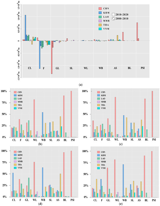
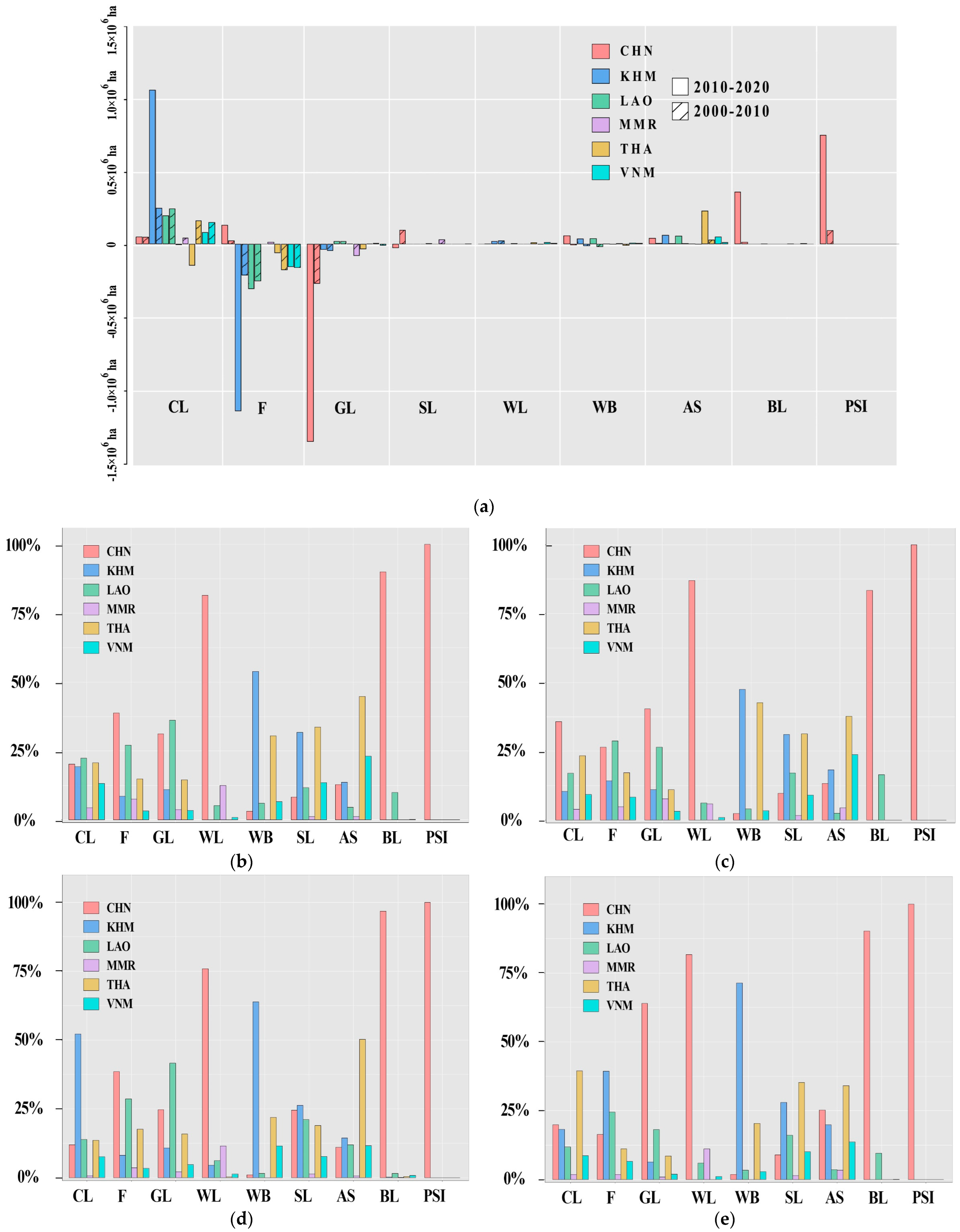
Figure 5.
Patterns of national differentiation in terms of: (a) net change for each LULC type during 2000–2020; (b) gain for each LULC type from 2000 to 2010; (c) loss for each LULC type from 2000 to 2010; (d) gain for each LULC type from 2010 to 2020; (e) loss for each LULC type from 2010 to 2020. CL means cultivated land, F means forest, GL means grassland, SL means shrubland, WL means wetland, WB means water body, AS means artificial surface, BL means bare land, PSI means permanent snow and ice. CHN: China; KHM: Cambodia; LAO: Laos; MMR: Myanmar; THA: Thailand; VNM: Vietnam.

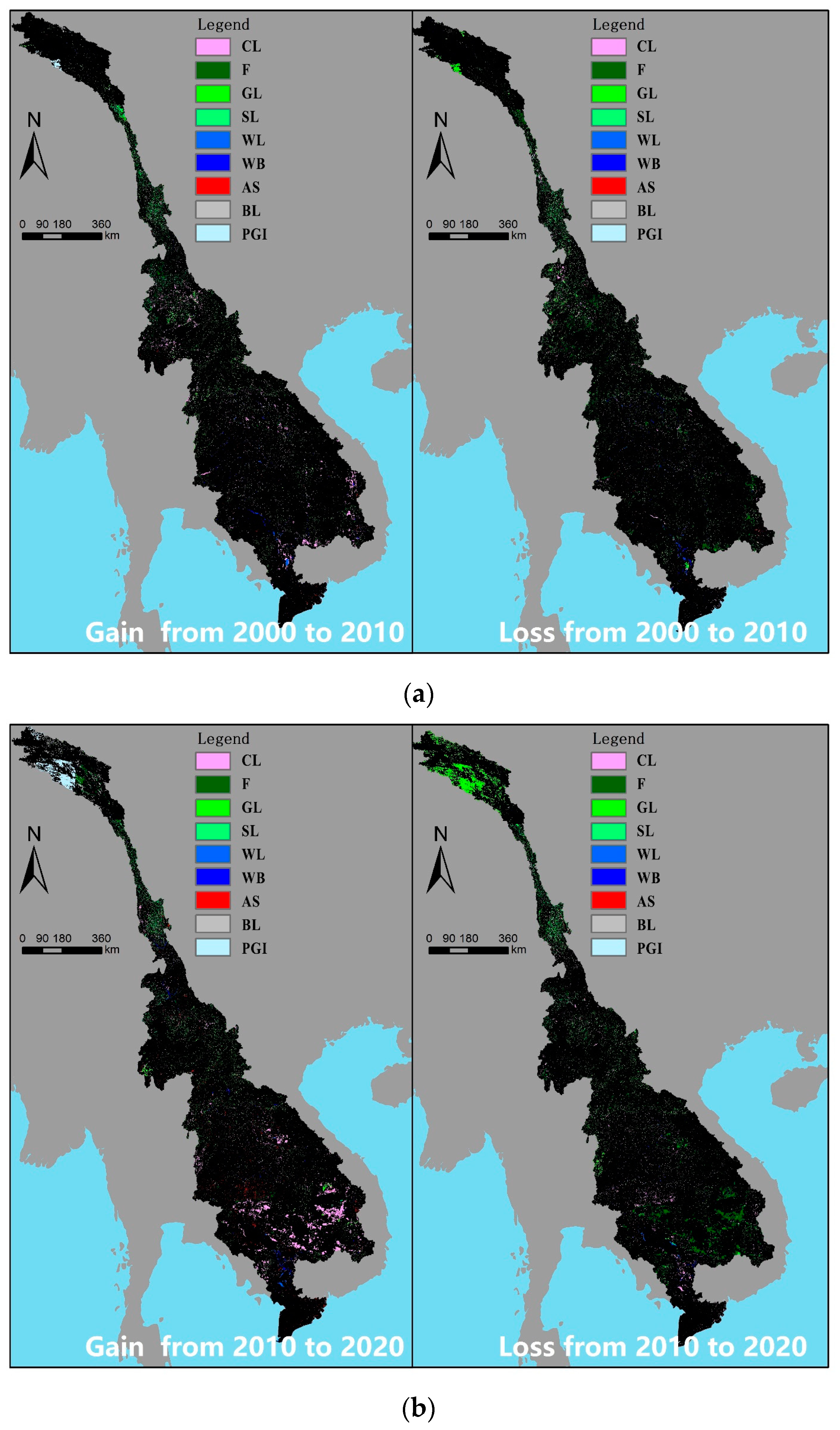
Figure 6.
LUCC across the LMRB: (a) gain and loss from 2000 to 2010; (b) gain and loss from 2010 to 2020. CL means cultivated land, F means forest, GL means grassland, SL means shrubland, WL means wetland, WB means water body, AS means artificial surface, BL means bare land, PSI means permanent snow and ice.
3.3. Conversion between Forests and Cultivated Land in the LMRB
In this study, the land use transition probability matrices reveal that the main direction of conversion within the LMRB over the two-decade period from 2000 to 2020 was the mutual conversion between cultivated land and forests. Figure 7 illustrates how forests and cultivated land were converted into other LULC types across different spatial units from 2000 to 2020, highlighting the dynamic changes in the LMRB’s landscape.
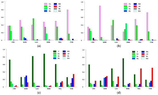
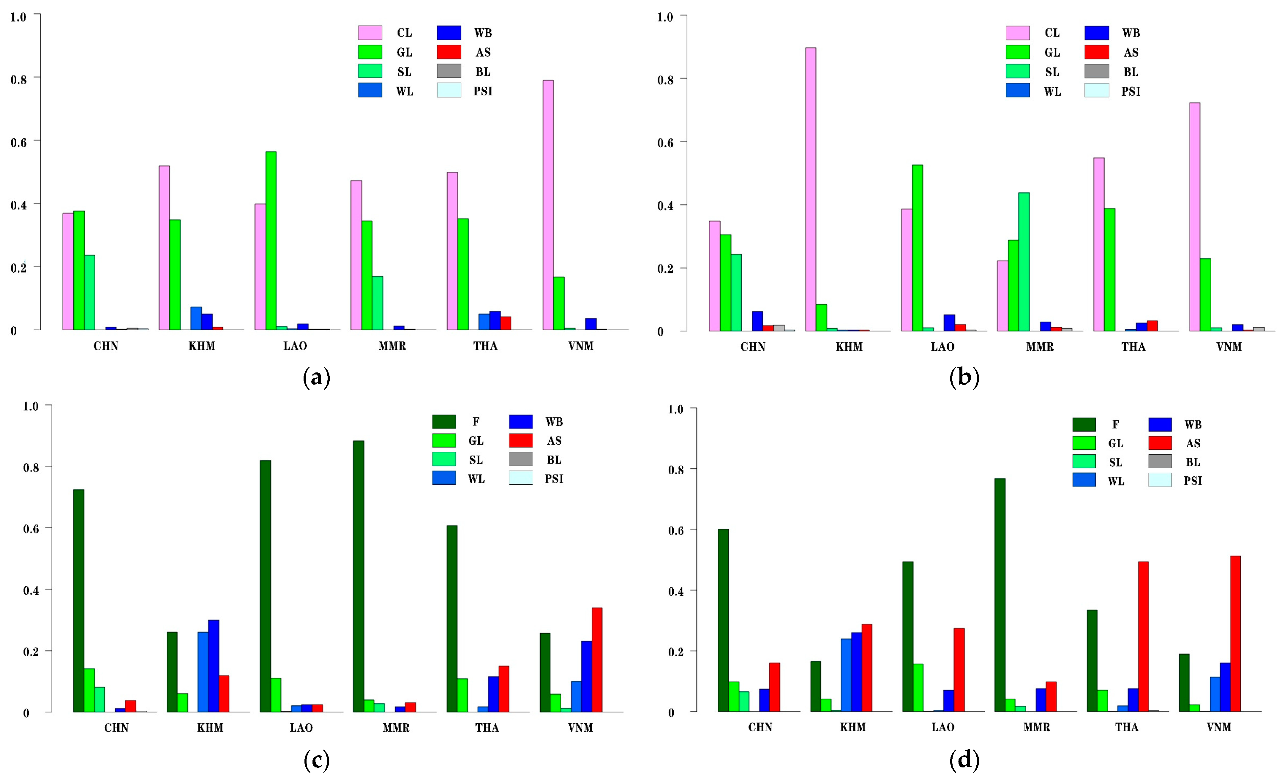
Figure 7.
The probability of conversion from forests to other LULC types during: (a) 2000–2010; (b) 2010–2020. The probability of conversion from cultivated land to other LULC types during: (c) 2000–2010; (d) 2010–2020. CL means cultivated land, F means forest, GL means grassland, SL means shrubland, WL means wetland, WB means water body, AS means artificial surface, BL means bare land, PSI means permanent snow and ice. CHN: China; KHM: Cambodia; LAO: Laos; MMR: Myanmar; THA: Thailand; VNM: Vietnam.
3.4. Mechanisms Impacting the Conversion from Cultivated Land to Forests
Before constructing a mathematical model to investigate the driving factors of the conversion from cultivated land to forests, several steps were taken to ensure the quality of the dataset and reduce bias. These steps included controlling sample balance and selecting significant explanatory variables through single-factor analysis. Firstly, the response variable in this study is a dichotomous variable, indicating the presence or absence of conversion from cultivated land to forests. In the first decade, 2112 samples were collected, consisting of 1050 positive cases and 1062 negative cases. In the second period, 1200 samples were collected, with 600 positive cases and 600 negative cases. The balance of positive and negative cases within the two sample sets ensures a reduced sample bias. Secondly, through the results of the single-factor binary logistic regression analysis (Table 5), it can be assumed that all the explanatory variables from X1 to X7 contribute to predicting the conversion from cultivated land to forests over the two decades analyzed, within the 95% confidence interval. Therefore, all the explanatory variables are included in the multi-factor logistic regression model.
Table 5.
The single-factor binary logistic regression analysis in two decades.
To investigate the factors influencing the conversion from cultivated land to forests, a mathematical model was constructed. Variables with strong correlations were excluded based on the results of the multi-factor analysis, and the best model was selected by comparing the overall accuracy of the models. Considering that each factor alone effectively predicted the response variable (as shown in Table 5), it was observed that the significance of the elevation factor’s influence on the response variable was less than 0.95 in the multi-factor logistic regression analyses from 2000 to 2010. Similarly, the significance of the elevation and slope factors’ influence on the response variable was less than 0.95 in the multi-factor logistic regression analyses from 2010 to 2020 (as shown in Table 6). Bivariate correlation analysis showed that the Spearman correlation coefficients between the variables in the two phases were lower than 0.7 (as shown in Table 7), with slope and elevation exhibiting the highest correlations of 0.696 and 0.695. It was observed that the correlation between slope and elevation influenced the results of the multi-factor logistic regression analyses. Therefore, Model 1 was constructed excluding the elevation factor, and Model 2 was constructed excluding the slope factor. The overall accuracy of Model 1 was higher than that of Model 2 (as shown in Table 8), suggesting that retaining the slope factor is better than retaining the elevation factor in predicting the conversion of cultivated land to forests.
Table 6.
The multi-factor binary logistic regression analysis in two decades.
Table 7.
Matrices of Spearman’s correlation coefficients between explanatory variables in two decades.
Table 8.
Two models concluded different explanatory variables over the two decades.
In Model 1, several factors were found to impact the conversion from cultivated land to forests. Firstly, the formulation of boundaries for the discretization of explanatory variables involved categorizing slopes into flat slope, gentle slope, slope, and steep slope, with dividing boundaries set at 5°, 15°, and 25°. Distances to the nearest main road and nearest tourist attraction were divided into categories of near distance, middle distance, and long distance, with dividing boundaries set at 9 km and 18 km. Changes in population density were categorized as either growth or nongrowth, based on whether they exceeded 0. Similarly, changes in nighttime light were divided into two categories: enhancement and non-enhancement (depending on whether they exceeded 0). Secondly, in the formulation of reference categories, logistic regression models were constructed using flat slope, long distance, non-growth, and non-enhancement as reference categories.
The computed pseudo-R-square values from the logistic regression models (Table 9) indicate that the models have a relatively good ability to explain the observed data. This study explored the specific patterns of each factor’s impact on the conversion from cultivated land to forests across three terms. Firstly, in terms of natural factors, the probability of cultivated land converting to forests on gentle slopes was 0.279-times as that on flat slopes, while the probability of conversion on steep slopes was 1.812-times as that on flat slopes in the first decade. However, no significant pattern could be observed in the second decade. Secondly, in terms of locational factors, the probability of conversion from cultivated land to forests within a middle distance to the nearest main road was 2.223-times as within a long distance. Similarly, the probability of conversion within a middle distance to the nearest tourist attraction was 1.533-times as within a long distance in the first decade. The consistent pattern continued in the second decade, with the probability of conversion within a middle distance to the nearest main road being 1.693-times as within a long distance, and the probability of conversion within the range of middle distance to the nearest tourist attraction being 2.379-times as within the range of long distance. Finally, in terms of socioeconomic factors, the probability of conversion from cultivated land to forests in growing regions was 1.458-times as in regions without growth. In the first decade, the probability of conversion in enhancing regions was 6.420-times as in regions without enhancement. Similarly, in the second decade, the pattern remained consistent, with the probability of conversion in growing regions being 2.916-times as in regions without growth, and the probability of conversion in enhancing regions being 3.062-times as in regions without enhancement.
Table 9.
Logistic regression models conducted for two decades to explain the impacting mechanisms of the conversion from cultivated land to forests.
4. Discussion
4.1. Classification of Countries within the Study Area
The results indicate that in the period from 2000 to 2020, the LMRB experienced a decrease in forests and an expansion in cultivated land. The mutual conversions between cultivated land and forests were the main transfer directions within the LMRB during this two-decade period. Forests play a crucial role in global ecosystems, carbon capture, ecological processes, and biodiversity conservation. Deforestation has historically been a major driver of LUCC, making it a topic of particular interest for LCS. Promoting ecological restoration in the LMRB requires collaborative efforts among the countries within the region. To determine which country within the LMRB places more emphasis on the conversion of cultivated land to forests, we classified the countries among the LMRB based on two conditions (Table 10). Condition one is if the forests within the spatial unit are converted into cultivated land the most. Condition two is if the cultivated land within the spatial unit is converted into forests the most.
Table 10.
Countries classified by two conditions.
Under condition one, based on trend in the conversions of forests, the six countries within the LMRB can be divided into two categories. The first category consists of countries that converted forests into cultivated land the most, promoting agricultural development and increasing food production to support their population. The second category consists of countries that converted forests into grasslands or shrublands the most, which represents ecological degradation. Under condition two, based on trend in the conversions of cultivated land, the six countries within the LMRB can also be divided into two categories. The first category consists of countries that converted cultivated land into forests the most, promoting sustainable agricultural development and improving regional ecological functions. The second category consists of countries that have converted cultivated land into artificial surfaces the most, reflecting the process of urbanization. In addition, Tonle Sap Lake occupies a large area of the country, and Cambodia’s cultivated land is converted more to water bodes rather than forests or artificial surfaces.
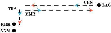
From 2010 to 2020, urban expansion and encroachment on cultivated land became the dominant trend in Thailand and Cambodia, replacing the previous trend of converting cultivated land into forests or water bodies from 2000 to 2010. Vietnam, located downstream from Thailand and Cambodia, experienced encroachment on cultivated land and city expansion as early as the first decade. In contrast, conversion from cultivated land to forests in China, Myanmar, and Laos improved the water quality by reducing the discharge of agricultural wastewater and increasing vegetation cover. This conversion results in cleaner water and enhanced water security for downstream cities along the Lancang–Mekong River, while also mitigating the adverse effects of urbanization on ecosystems in Thailand, Cambodia, and Vietnam. Despite these positive effects brought by upstream regions to the downstream regions, the government’s land administration needs to pay more attention to the protection of natural resources within the LMRB due to the acceleration of urban expansion in Thailand, Cambodia, and Vietnam over two decades from 2000 to 2020.
4.2. Implications of the Findings for Policy Development
Serving as crucial carbon sinks, declines in forests and grasslands during the two decades from 2000 to 2020 can significantly reduce carbon sequestration and storage capacities, as well as weakening the whole ecological services within the LMRB. There are two ways of increasing forest cover. The first is to establish protected areas for forests. However, resources from managers are limited. It is important to decide where to focus budgets for law enforcement. So, identifying areas more vulnerable to forest degradation or deforestation is a key aspect. A previous study explored the driving factors affecting deforestation. Zeng et al. found that [21] annual forest loss is significantly correlated with the global corn price. That means that food production in South-East Asia is not solely focused on the food needs of the region’s population. Agricultural expansion is a key driver of forest loss in Nan Province. Bavaghar proposed that deforestation is a function of slope, distance to roads, and residential areas using the logistic regression model [36]. Linkie et al. found that between 1985 and 1992, forests located at lower elevation and close to roads were the most vulnerable to clearance. These factors were also significant between 1992 and 1999, along with the distance to newly created logging roads [37]. The second way is to convert other LULC types to forests to increase forest cover. As two LULC types strongly linked to human activities, cultivated land accounts for a larger proportion of the total basin area compared to artificial surfaces. As shown above, conversion from cultivated land to forests has the highest probability of all possibilities in the past two decades when converting cultivated land to other LULC types. In summary, exploring the factors contributing to the conversion from cultivated land to forests in the LMRB is worthy of enhancing ecological services in the LMRB. Further, exploring the factors affecting the conversion from cultivated land to forests concretely helps to develop accurate and enforceable policy. We used a logistic regression model to explore the driving factors affecting this process.
The results indicate that several factors impact the conversion from cultivated land to forests, including slope, distance to the nearest main road, distance to the nearest tourist attraction, change in population density, and change in nighttime light. In terms of natural factors, the probability of the conversion from cultivated land follows a U-shaped curve in relation to slope. This means that compared to regions with a gentle slope, there is a larger probability for the region with a flat slope or steep slope to be converted from cultivated land to forests. When the policy of converting cultivated land into forests is implemented, the probability of the conversion from cultivated land to forests happening on the extensive flat slope is greater. Additionally, farmers are more inclined to abandon areas with steep slopes, where soil erosion is more serious and cultivated land management is difficult. Meanwhile, the government prefers to include cultivated land with a slope greater than 25° in the priority areas for the implementation of the policy of returning cultivated land to forests. In terms of locational factors, the relationship between the traffic conditions and the probability of conversion from cultivated land to forests is positive, while there is an optimal distance between cultivated land and the nearest tourist attraction with the highest probability of conversion into forests. The closer the cultivated land is to the nearest main road, the greater the probability of conversion from cultivated land to forests. The middle distance between the cultivated land and the nearest tourist attraction is the optimal distance, and, in this study, the middle distance is defined with a range from 9 km to 18 km. Here, it enjoys the advantage of closer proximity to the natural environment and, at the same time, can obtain the economic opportunities brought by the development of tourism. In terms of socioeconomic factors, the conversion from cultivated land to forests is significantly associated with human interventions. The conversion from cultivated land to forests is more likely to occur in areas where the population grows and the light is enhanced at nighttime. Therefore, relevant government departments can intervene in the direction of cultivated land conversion in an effective way, such as exploring suitable economic incentives and conducting rational land use planning.
4.3. Limitations and Future Work
The ecological governance of transboundary watersheds is procedurally complex, and providing policy advice universally is not feasible. For example, land is an important means of production, and governments should formulate different land use policies based on different ownerships systems. Theoretically, the means of production are publicly owned in socialist countries and privately owned in capitalist countries. In Thailand, the land law was amended in 2008 through the Land Law Amendment Act (No. 12). The current land system in Thailand is based on private ownership, and land throughout the country is divided into three categories: crown-owned, state-owned, and privately owned. The recent changes in Thailand’s land system have led to the establishment of private land ownership, which has significantly contributed to the country’s modernization process. The Land Law in Cambodia was promulgated in 1992 and amended in August 2001. The amended Land Law focuses on provisions related to the protection of immovable property. At the end of 2009, the Cambodian National Assembly approved the law on land expropriation, granting the government the authority to expropriate land in the interest of social and public welfare. The law defines public interest activities as the construction, rehabilitation, protection, or expansion of infrastructure projects, development of defense and civil security buildings, border crossing posts, facilities for research and development of natural resources, as well as oil pipelines and gas networks. According to the Constitution of Vietnam, land is collectively owned by the people, and the State acts as the representative of the owners, managing the land in a unified manner. Vietnamese law does not recognize private ownership of land.
Our research can contribute to the development of national policies for converting cultivated land to forests. This study not only explored the factors influencing the conversion of cultivated land to forests but also delved into the extent and direction of the influence of these factors on the conversion process. Compared to discriminant analysis, logistic regression analyses are less demanding in terms of the distribution of explanatory variables [38]. Logistic regression models are particularly useful when dealing with qualitative or dummy variables. Hosmer et al. authored a book providing guidance on the application of logistic regression [39]. Two of the authors are biostatisticians, while the other is an academic in the Department of Mathematical Sciences. Assessing the performance of the model is a crucial step in the modelling process. The area under the ROC curve is a reliable indicator for assessing the performance of the model, in addition to overall accuracy [40]. However, there are still some shortcomings, such as the large size of the study area and the overall accuracy and AUC value of the model not being particularly satisfactory. Future studies could focus on smaller spatial units within the study area and employ alternative models that achieve higher overall precision by fitting the explanatory and response variables. In addition, climatic factors such as temperature and precipitation were not considered in the analyses. An AUC value above 0.7 or below 0.3 indicates that the model has good categorization performance. Although the overall accuracy and AUC value of the logistic regression model in this study exceeded 0.7, the performance can be improved by adding additional variables. Factors associated with returning cultivated land to forests may change over time, so spatial models should be updated periodically to reflect these changes.
5. Conclusions
This study considers the spatio-temporal patterns of LUCC within the study area from 2000 to 2020. To promote forest restoration, binary logistic regression models were applied to analyze the factors influencing the conversion from cultivated land to forests in the LMRB during 2000–2020. The results indicate that areas with a slope ranging from 5° to 15° exhibit the lowest probability of conversion, while cultivated land located 9 km to 18 km from the nearest tourist attraction has the highest probability. The conversion process demonstrates a positive correlation with traffic conditions and is significantly influenced by human interventions. Meanwhile, the models we built were evaluated using the ROC curve. The models we built possess a high degree of universality, despite the relatively huge size of the study area, resulting in a relatively low AUC value. Future studies could apply similar modeling approaches to different regions within the LMRB. The findings in this research can inform decision-making processes in the LMRB, encouraging the governments of various countries within the LMRB to establish mutual incentives and effectively implement land use policies that promote increased forest cover. This is crucial for mitigating water disasters, soil erosion, and biodiversity loss, ensuring the sustainable development of the region while protecting its natural resources and ecological systems.
Author Contributions
Methodology, F.L., Y.L., S.L. and Z.C.; software, F.L.; validation, F.L.; formal analysis, F.L.; data curation, F.L.; writing—original draft preparation, F.L., Y.L., S.L., G.L., Z.C. and Z.G.; writing—review and editing, F.L., Y.L., S.L., G.L., Z.C. and Z.G.; visualization, F.L.; supervision, Y.L., S.L., G.L. and Z.C.; project administration, Y.L.; funding acquisition, Y.L. All authors have read and agreed to the published version of the manuscript.
Funding
This research was funded by the National Natural Science Foundation of China, grant numbers 42271180 and 41871114.
Institutional Review Board Statement
Not applicable.
Informed Consent Statement
Not applicable.
Data Availability Statement
Data are contained within the article.
Acknowledgments
The authors would like to express their sincere gratitude to the United States Geological Survey (USGS), OpenStreetMap (OSM) and the China National High-Tech Research and Development Programme (NHRDP) for providing the DEM data, data on locational elements and GlobeLand30 data. Meanwhile, the authors extend their heartfelt appreciation to Yu’s team and Oak Ridge National Laboratory for providing the nighttime light data and population density data for the years 2000, 2010, and 2020, which were used in this study.
Conflicts of Interest
The authors declare no conflicts of interest.
References
- Wang, J.; He, T.; Guo, X.; Liu, A. Study on Land Degradation Trend by Applying Logistic Multivariate Regression Model in Northwest Region of Beijing. Prog. Geogr. 2005, 24, 25–34+134. [Google Scholar]
- Ge, R.; Ma, C. Analysis on Land Use Change and Driving Factors of Lake Wetland in Arid Plateau. Res. Soil Water 2022, 29, 376–385. [Google Scholar] [CrossRef]
- Li, Z.-T.; Li, M.; Xia, B.-C. Spatio-Temporal Dynamics of Ecological Security Pattern of the Pearl River Delta Urban Agglomeration Based on LUCC Simulation. Ecol. Indic. 2020, 114, 106319. [Google Scholar] [CrossRef]
- Li, B.; Bi, J.; Tian, Y. Effects of Land Use Change on Ecosystem Service Value in the Heavy Polluted Area in Taihu Lake Basin. Sci. Geogr. Sin. 2012, 32, 471–476. [Google Scholar] [CrossRef]
- Wang, J.; Wu, Z.; Li, S.; Wang, S.; Zhang, X.; Gao, Q. Coastline and Land Use Change Detection and Analysis with Remote Sensing in the Pearl River Estuary Gulf. Sci. Geogr. Sin. 2016, 36, 1903–1911. [Google Scholar] [CrossRef]
- Yu, X.; Li, J.; Liu, Q.; Wu, Y.; Sun, Q.; Gao, Y. Land Use Structure Optimization Research Based on Nitrogenand Phosphorus Output Risky Control in Small Watershed. Sci. Geogr. Sin. 2013, 33, 1111–1116. [Google Scholar] [CrossRef]
- Liu, S.; Li, X.; Chen, D.; Duan, Y.; Ji, H.; Zhang, L.; Chai, Q.; Hu, X. Understanding Land Use/Land Cover Dynamics and Impacts of Human Activities in the Mekong Delta over the Last 40 Years. Glob. Ecol. Conserv. 2020, 22, e00991. [Google Scholar] [CrossRef]
- Zhu, X.; Yang, Q.; Ding, Z.; Li, C.; Tang, L.; Chen, B. Ecosystem landscape pattern change and its response to climate in desert steppe of Inner Mongolia. Chin. J. Ecol. 2023, 42, 748–758. [Google Scholar] [CrossRef]
- Zhang, X.; Kang, T.; Wang, H.; Sun, Y. Analysis on Spatial Structure of Landuse Change Based on Remote Sensing and Geographical Information System. Int. J. Appl. Earth Obs. Geoinf. 2010, 12, S145–S150. [Google Scholar] [CrossRef]
- Hao, B.; Han, X.; Ma, M.; Liu, Y.; Li, S. Research Progress on the Application of Google Earth Engine in Geoscience and Environmental Sciences. Remote Sens. Technol. Appl. 2018, 33, 600–611. [Google Scholar]
- Sang, X.; Guo, Q.; Wu, X.; Fu, Y.; Xie, T.; He, C.; Zang, J. Intensity and Stationarity Analysis of Land Use Change Based on CART Algorithm. Sci. Rep. 2019, 9, 12279. [Google Scholar] [CrossRef] [PubMed]
- Peng, B.; Chen, D.; Li, W.; Wang, Y. Stability of Landscape Pattern of Land Use:A Case Study of Changde. Sci. Geogr. Sin. 2013, 33, 1484–1488. [Google Scholar] [CrossRef]
- Richards, D.R.; Friess, D.A. Rates and Drivers of Mangrove Deforestation in Southeast Asia, 2000–2012. Proc. Natl. Acad. Sci. USA 2016, 113, 344–349. [Google Scholar] [CrossRef] [PubMed]
- Grainger, A. National Land Use Morphology: Patterns and Possibilities. Geography 1995, 80, 235–245. [Google Scholar]
- Liang, Y.; Zeng, J.; Sun, W.; Zhou, K.; Zhou, Z. Expansion of Construction Land along the Motorway in Rapidly Developing Areas in Cambodia. Land Use Policy 2021, 109, 105691. [Google Scholar] [CrossRef]
- He, D.; Jin, F.; Zhou, J. The Changes of Land Use and Landscape Pattern Based on Logistic-CA-Markov Model—A Case Study of Beijing-Tianjin-Hebei Metropolitan Region. Sci. Geogr. Sin. 2011, 31, 903–910. [Google Scholar] [CrossRef]
- Yu, M.; Sun, J.; Yang, W.; Xie, F.; Lyu, J. Evolution of Land Use Degree in Gansu Province Based on Bayesian Hierarchical Spatio-temporal Model. Sci. Geogr. Sin. 2022, 42, 918–925. [Google Scholar] [CrossRef]
- Achard, F.; Beuchle, R.; Mayaux, P.; Stibig, H.; Bodart, C.; Brink, A.; Carboni, S.; Desclée, B.; Donnay, F.; Eva, H.D.; et al. Determination of Tropical Deforestation Rates and Related Carbon Losses from 1990 to 2010. Glob. Change Biol. 2014, 20, 2540–2554. [Google Scholar] [CrossRef]
- Margono, B.A.; Potapov, P.V.; Turubanova, S.; Stolle, F.; Hansen, M.C. Primary Forest Cover Loss in Indonesia over 2000–2012. Nat. Clim. Change 2014, 4, 730–735. [Google Scholar] [CrossRef]
- FAO. The State of the World’s Forests in 2022; FAO: Rome, Italy, 2022; ISBN 978-92-5-136001-9. [Google Scholar]
- Zeng, Z.; Gower, D.B.; Wood, E.F. Accelerating Forest Loss in Southeast Asian Massif in the 21st Century: A Case Study in Nan Province, Thailand. Glob. Change Biol. 2018, 24, 4682–4695. [Google Scholar] [CrossRef]
- Yun, X.; Tang, Q.; Xu, X.; Zhou, Y.; Liu, X.; Wang, J.; Sun, S. Impact of climate change on water resource cooperation between the upstream and downstream of the Lancang-Mekong River basin. Clim. Change Res. 2020, 16, 555–563. [Google Scholar]
- Zhou, Y.; Li, X.; Liu, Y. Land Use Change and Driving Factors in Rural China during the Period 1995–2015. Land Use Policy 2020, 99, 105048. [Google Scholar] [CrossRef]
- Lazar, M. Shedding Light on the Global Distribution of Economic Activity. Open Geogr. J. 2010, 3, 147–160. [Google Scholar] [CrossRef]
- Wang, Z.; Liu, J.; Li, J.; Meng, Y.; Pokhrel, Y.; Zhang, H. Basin-Scale High-Resolution Extraction of Drainage Networks Using 10-m Sentinel-2 Imagery. Remote Sens. Environ. 2021, 255, 112281. [Google Scholar] [CrossRef]
- Munia, H.; Guillaume, J.H.A.; Mirumachi, N.; Porkka, M.; Wada, Y.; Kummu, M. Water Stress in Global Transboundary River Basins: Significance of Upstream Water Use on Downstream Stress. Environ. Res. Lett. 2016, 11, 014002. [Google Scholar] [CrossRef]
- Mora, B.; Romijn, E.; Herold, M. Monitoring Progress towards Sustainable Development Goals. In Proceedings of the 5th GEOSS Science and Technology Stakeholder Workshop—Linking the Sustainable Development Goals to Earth Observations, Models and Capacity Building, Berkeley, CA, USA, 9–10 December 2016. [Google Scholar]
- Chen, J.; Cao, X.; Peng, S.; Ren, H. Analysis and Applications of GlobeLand30: A Review. ISPRS Int. J. Geo-Inf. 2017, 6, 230. [Google Scholar] [CrossRef]
- GlobeLand30 Data Platform. Available online: http://www.globallandcover.com (accessed on 2 February 2024).
- Chen, J.; Chen, J.; Liao, A.; Cao, X.; Chen, L.; Chen, X.; He, C.; Han, G.; Peng, S.; Lu, M.; et al. Global Land Cover Mapping at 30m Resolution: A POK-Based Operational Approach. ISPRS J. Photogramm. Remote Sens. 2015, 103, 7–27. [Google Scholar] [CrossRef]
- Chen, Z.; Yu, B.; Yang, C.; Zhou, Y.; Yao, S.; Qian, X.; Wang, C.; Wu, B.; Wu, J. An Extended Time Series (2000–2018) of Global NPP-VIIRS-like Nighttime Light Data from a Cross-Sensor Calibration. Earth Syst. Sci. Data 2021, 13, 889–906. [Google Scholar] [CrossRef]
- Pontius, R.G.; Shusas, E.; McEachern, M. Detecting Important Categorical Land Changes while Accounting for Persistence. Agric. Ecosyst. Environ. 2004, 101, 251–268. [Google Scholar] [CrossRef]
- Sun, Z.; Scott, I.; Bell, S.; Zhang, X.; Wang, L. Time Distances to Residential Food Amenities and Daily Walking Duration: A Cross-Sectional Study in Two Low Tier Chinese Cities. Int. J. Environ. Res. Public Health 2021, 18, 839. [Google Scholar] [CrossRef]
- Zhou, Z.-R.; Wang, W.-W.; Li, Y.; Jin, K.-R.; Wang, X.-Y.; Wang, Z.-W.; Chen, Y.-S.; Wang, S.-J.; Hu, J.; Zhang, H.-N.; et al. In-Depth Mining of Clinical Data: The Construction of Clinical Prediction Model with R. Ann. Transl. Med. 2019, 7, 796. [Google Scholar] [CrossRef]
- Fawcett, T. An Introduction to ROC Analysis. Pattern Recognit. Lett. 2006, 27, 861–874. [Google Scholar] [CrossRef]
- Pir Bavaghar, M. Deforestation Modelling Using Logistic Regression and GIS. J. For. Sci. 2015, 61, 193–199. [Google Scholar] [CrossRef]
- Linkie, M.; Smith, R.J.; Leader-Williams, N. Mapping and Predicting Deforestation Patterns in the Lowlands of Sumatra. Biodivers. Conserv. 2004, 13, 1809–1818. [Google Scholar] [CrossRef]
- Press, S.J.; Wilson, S. Choosing between Logistic Regression and Discriminant Analysis. J. Am. Stat. Assoc. 1978, 73, 699–705. [Google Scholar] [CrossRef]
- Hosmer, D.W., Jr.; Lemeshow, S.; Sturdivant, R.X. Applied Logistic Regression; John Wiley & Sons: Hoboken, NJ, USA, 2013. [Google Scholar]
- Bradley, A.P. The Use of the Area under the ROC Curve in the Evaluation of Machine Learning Algorithms. Pattern Recognit. 1997, 30, 1145–1159. [Google Scholar] [CrossRef]
Disclaimer/Publisher’s Note: The statements, opinions and data contained in all publications are solely those of the individual author(s) and contributor(s) and not of MDPI and/or the editor(s). MDPI and/or the editor(s) disclaim responsibility for any injury to people or property resulting from any ideas, methods, instructions or products referred to in the content. |
© 2024 by the authors. Licensee MDPI, Basel, Switzerland. This article is an open access article distributed under the terms and conditions of the Creative Commons Attribution (CC BY) license (https://creativecommons.org/licenses/by/4.0/).