Evaluation of Soil Hydraulic Properties in Northern and Central Tunisian Soils for Improvement of Hydrological Modelling

Abstract

The hydrological cycle is strongly affected by climate changes causing extreme weather events with long drought periods and heavy rainfall events. To predict the hydrological functioning of Tunisian catchments, modelling is an essential tool to estimate the consequences on water resources and to test the sustainability of the different land uses. Soil physical properties describing water flow are essential to feed the models and must therefore be determined all over the watershed. A simple but robust ring infiltration method combined with particle size distribution (PSD) analysis (BEST method) was used to evaluate and derive the retention properties and the hydraulic conductivities. Physically based and statistical pedotransfer functions based on PSD were compared to test their potential use for different types of Tunisian soils. The functional sensitivity of these parameters was assessed by employing the Hydrus-1D software (PC Progress, Prague, Czech Republic) for water balance computations. This evaluation process involved testing the responsiveness and accuracy of the parameters in simulating various water balance components within the model. The evaluation of soil hydraulic parameters across the three used models highlighted significant variations, demonstrating distinct characteristics in each model. While notable differences were evident overall, intriguing similarities emerged, particularly regarding saturated hydraulic conductivity between BEST and Rosetta, and the shape parameter (n) between Arya–Paris and Rosetta. These parallels indicate shared hydraulic properties among the models, underscoring areas of agreement amid their diverse results. Significant differences were shown for scale parameter $\alpha$ for the various methods employed. Marginal differences in evaporation and drainage were observed between the BEST and Arya–Paris methods, with Rosetta distinctly highlighting a disparity between physically based models and statistical models.

1. Introduction

Amongst the different soil hydraulic parameters, saturated hydraulic conductivity ($K_s$) is a chief parameter; it has a direct influence on infiltration rate. It is often used to estimate the partitioning of rainfall between infiltration and surface flow [1], thus impacting the runoff regime and soil erosion during high-intensity rainfall events [2,3]. During the initial stage of infiltration in dry soils, water flow is primarily influenced by sorptivity, which represents the capacity of a porous medium to absorb water by capillarity and which plays a crucial role in the overall infiltration process, as highlighted in studies by Lassabatere et al. [4,5]. Therefore, the soil water retention properties relating water pressure head h to volumetric water content $\theta \left(h\right)$ are also of great importance for hydrological modeling. Typically, soil hydraulic properties, particularly saturated hydraulic conductivity ($K_s$), exhibit significant spatial heterogeneity [6,7,8]. It is reported to have the greatest statistical variability among different soil hydrological properties [9,10,11,12,13,14] and can be induced by many factors such as soil texture, structure, organic matter content, hydrophobicity, and compaction [15,16]. These factors interact in complex ways, resulting in spatial variability in saturated hydraulic conductivity across different soil types and landscapes with varying intensities across different scales [17,18,19]. According to Libohova et al. [20], the success of predictions when modelling hydrological processes depends on the accurate representation of the spatial and temporal variability of soil hydrological attributes and the main external factors [9,21] such as soil water dynamics which is mainly influenced by the natural and anthropogenic processes predominantly at the surface layer [10,22,23,24,25,26,27]. One can explore various approaches to determine soil hydraulic conductivity. Broadly, these methods fall into three categories: laboratory-based, field-based, and empirical techniques [28]. Laboratory and field methods typically offer higher accuracy, albeit at the expense of time and cost. Conversely, empirical methods are known for their swiftness and simplicity. To circumvent the laborious and time-intensive process of measuring unsaturated soil properties [29], pedotransfer functions (PTFs) are increasingly employed [30,31]. PTFs are invaluable tools in soil science, offering a means to predict soil hydraulic properties through easily obtainable soil characteristics [32,33]. These properties play a pivotal role in optimizing water management across various scales, from catchment to continental modelling [34]. While significant aspects regarding the importance and use of soil hydraulic parameters through PTFs have been revealed, controversies persist regarding the accuracy of PTFs in predicting soil hydraulic parameters. Discrepancies between measured values and those predicted by PTFs raise questions about the reliability of these methods. Also, ambiguities surround the variability in predictions made by different PTFs, indicating inconsistencies in estimating soil hydraulic properties across diverse soil types and conditions. Addressing these issues is essential to enhance the reliability and applicability of PTFs in determining soil hydraulic parameters effectively.

Two areas are chosen, one in the northern region and the other in the central region of Tunisia. They both hold significant agronomical and hydrological importance within the country’s strategic planning. They also highlight the challenges of managing water resources sustainably in semi-arid regions and play a vital role in intensive irrigated vegetable and fruit production. They offer valuable insights into agronomical practices, water management strategies, and sustainable development initiatives crucial for Tunisia’s overall agricultural and hydrological planning. PTFs provide a cost-effective and straightforward method to estimate soil hydraulic properties, thereby enhancing water management efficiency for agricultural practices.

These functions establish a link between desired soil hydraulic parameters and readily available soil properties using a soil hydraulic model [35,36]. Developed and validated across diverse soil types and conditions, PTFs enable estimation in varied contexts [37]. Recent research has focused on evaluating and improving PTFs for specific soil types and conditions, but there has also been a growing interest in a new category of methods that adopt a hybrid approach, incorporating both empirical models and experimental data [38,39,40]. Additionally, efforts have been made to develop ensemble pedotransfer functions to derive hydraulic properties for different soil types. These advancements in PTFs contribute to developing more accurate and reliable soil hydraulic property estimates, ultimately improving water management strategies and decision-making processes. Pedotransfer functions are mostly based on empirical relationships derived from databases like UNSODA [41] or ROSETTA [42] relating saturated hydraulic conductivity and retention properties to soil texture [28,43,44,45]. Conversely, physically based models that establish connection between particle size distribution and pore size distribution are widely developed [46,47,48]. Comparison of different evaluation methods of soil water parameters with PTFs or other methods often consists in field or laboratory experiments to compare the actual values of these parameters and evaluate them in relation to a reference method [49]. Nevertheless, few of them address the problem of the final use of these parameters [33,50,51]. This study aims to evaluate the functional sensitivity of the method employed to derive soil hydraulic properties in the northern and central regions of Tunisia. In addition to merely evaluating these functions through different methods, we also consider their actual impact on water flow evaluation under specific climate conditions. This assessment involves computing the water balance using HYDRUS-1D [52].

2. Materials and Methods

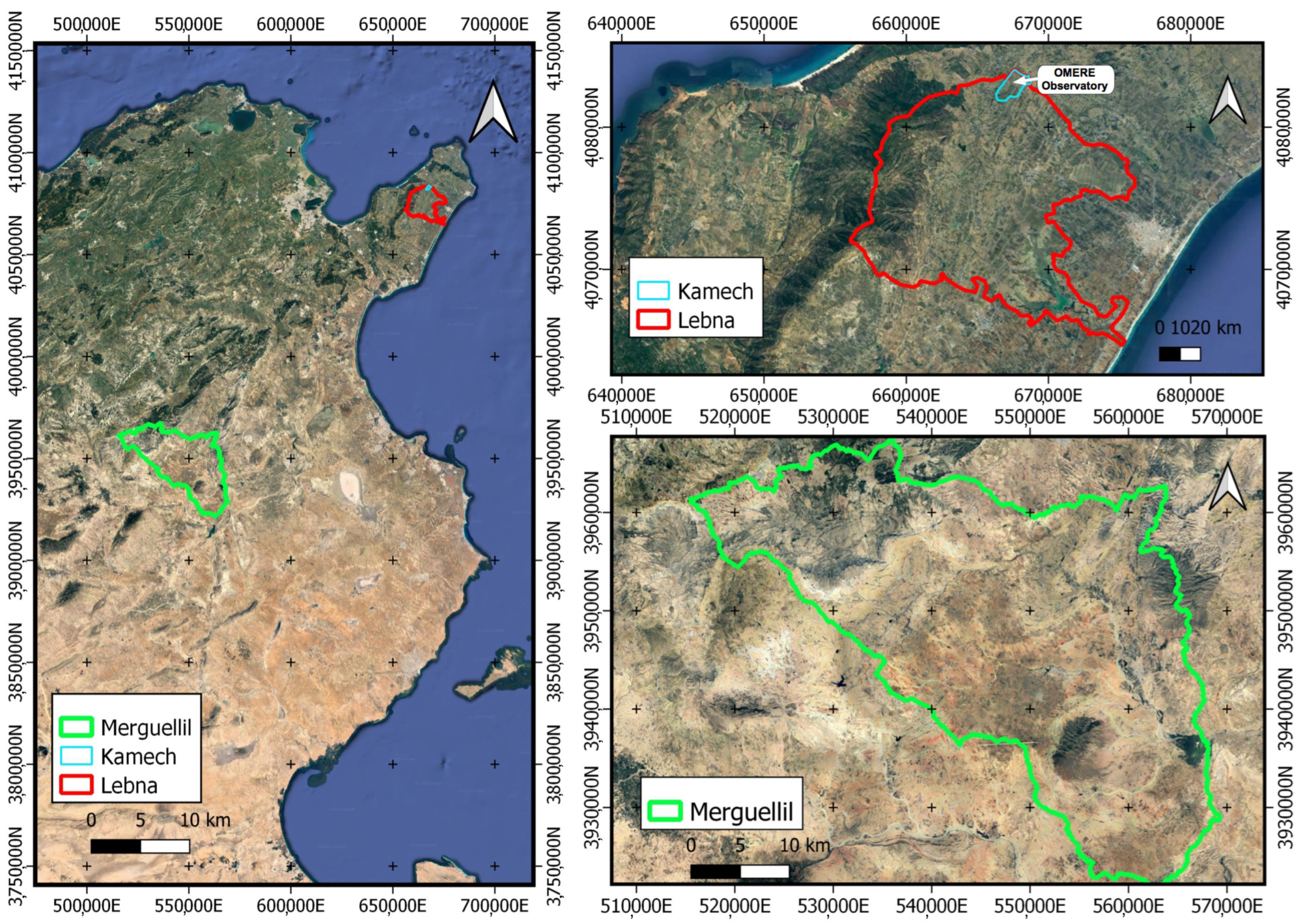
2.1. Study Area

This study is part of a wider regional research program about water management in Mediterranean agricultural hydro-systems (PRIMA, ALTOS). It is located in two distinct Tunisian watersheds in Cap Bon and in Central Tunisia (Figure 1). The study area is classified under the Köppen climate classification system as a region with a Mediterranean semi-arid climate, typically denoted by the code “Csa”. This classification indicates that the area experiences hot, dry summers accompanied by mild, humid winters, reflecting the characteristic seasonal patterns of temperature and precipitation found in Mediterranean climates [53]. The Lebna watershed is located in the northern part of the Cap Bon (36°53′00.0″ N 10°58′00.0″ E) and covers an area of 210 ${\mathrm{km}}^2$. The area presents Alfisols, Entisols, and Vertisols. The area’s climate is characterized by a rainfall below 500 mm per year and an evaporative demand of around 1200 mm. The watershed experiences a wet regime at higher altitudes with rainfall exceeding 700 mm per year, transitioning to a semi-arid climate downstream where precipitation levels drop below 500 mm annually. The vegetation cover in the Lebna watershed consists of scrubland and forest in the central part, hilly reliefs with a mix of crops and rangelands, and flat areas with annual crops and orchards downstream. The vegetation types in this watershed contribute to soil conservation and ecosystem services. The watershed extends from the Jebel Abderrahmane to the Korba Laguna which is represented by a mountainous and hilly landscape upslope and a flat plain near the mouth. The Kamech watershed is a 2.63 ${\mathrm{km}}^2$ sub-catchment of the Lebna watershed (36°52′48.0″ N 10°52′48.0″ E) and has been monitored since 2004 as part of the OMERE Mediterranean Observatory for Land and Water [54].

The upstream part of the Merguellil watershed is located in central Tunisia (35°34′02.3″ N 9°44′06.4″ E) and is characterized by high space and temporal rainfall variability and high evaporation rates. Annual means vary between 300 mm in the plain and 500 mm in the highest parts. The annual mean temperature is 19.6 °C, with a maximum of 48 °C in August and a minimum of −2 °C in January. The mean annual potential evapotranspiration is 1430 mm/year with a maximum of 1600 mm/year. The upstream basin has a surface area of 1200 ${\mathrm{km}}^2$. Half of it is cultivated with annual crops (wheat) and trees (olive and almond). Grazing lands cover 30 per cent, forests 19 per cent, and urban areas 1 per cent. The altitude of the upstream Merguellil watershed varies between 200 and 1200 m, with an average of about 500 m. The watershed is delimited by a succession of djebels (mountainous ridges), and the El Haouareb dam is anchored in two lateral djebels (Aïn El Rhorab and El Haouareb). The area is affected by various environmental issues. It experiences a continuous decline in the water table due to over-exploitation and faces an accentuation of the water deficit because of climate change and the presence of numerous illegal boreholes and poor soil management [55].

2.2. Experimental Design

This study was conducted in both watersheds covering several soil types belonging to different soil textural classes as depicted in Figure 2.

The soil hydraulic properties were estimated in 31 locations (3 replications) with three different methods. Arya–Paris and Rosetta are mainly based on the analysis of particle size distribution (PSD) and bulk density [28]. For the BEST method [38,39,40], the PSD analysis is complemented by an in situ single-ring infiltration experiment (Beerkan) to more accurately derive hydraulic conductivity. The soil hydraulic parameters issued from the different methods were later submitted to statistical analysis to determine whether there was any significant difference between them. These obtained parameters served as inputs for HYDRUS-1D which takes into consideration the main weather condition boundaries: experimental rainfall and reference evapotranspiration ($E{T}_0$) data collected in Kamech station used to simulate the water flows. At this step, the statistical analysis serves to show whether the determined soil hydraulic parameters with different methods have any impact on the final results issued from the simulation. For each measure, a soil sample was taken for particle size distribution analysis and another sample was taken for bulk density determination. Water initial content was also measured for each measurement location. The principal inputs and outputs, as well as the methods used, are represented in Figure 3.

2.3. Estimation of Soil Hydraulic Properties

Water flow in the vadose zone is well described by Richards’ equation [56] which, for 1D vertical flow, is

$$\frac{\partial \theta }{\partial t}=\frac{\partial }{\partial t}\left[K\left(\theta \right)\left(\frac{\partial h}{\partial z}+1\right)\right]-S$$

(1)

where $K\left(\theta \right)$ is the unsaturated hydraulic conductivity, $\theta$ is the volumetric water content, h is the water pressure head, S is the sink term representing the root water uptake. In order to solve this equation, the basic unsaturated soil properties need to be determined, namely the retention curve and the hydraulic conductivity described, respectively, by van Genuchten functions [57],

$$S_e={\left(1+{\left(\alpha h\right)}^n\right)}^{-m}=\frac{\theta -{\theta }_r}{{\theta }_s-{\theta }_r}$$

(2)

and

$$K\left(\theta \right)=K_s·{S_e}^l{\left[1-{\left(1-{S_e}^{1/m}\right)}^m\right]}^2$$

(3)

where $S_e$ [–] is the effective saturation, $\theta$ [${\mathrm{L}}^3·{\mathrm{L}}^{-3}$] is the volumetric water content, ${\theta }_r$ and ${\theta }_s$ are the residual at saturated water content, n [–] and m [–] are shape parameters, $\alpha$ [${\mathrm{L}}^{-1}$] is the scale parameter, $K_s$ [$\mathrm{L}·{\mathrm{T}}^{-1}$] is the saturated hydraulic conductivity and l [–] is an empirical parameter usually set to 1/2. Parameter m is a function of parameter n:

$$m=1-k/n$$

where k is an integer usually chosen to be 1 for Mualem conditions [58] or sometimes 2 for Burdine conditions [59]. However, hydraulic conductivity is also often described by the Brooks and Corey [60] expression:

$$K\left(\theta \right)=K_s·{S_e}^{\eta }$$

(4)

where $\eta$ is an empirical shape parameter.

2.4. The Empirical Method: ROSETTA

One of the most common methods to derive soil hydraulic properties is to use pedotransfer functions (PTFs). They represent empirical models based on large soil databases to estimate soil hydraulic properties for common and easily available soil information such as soil texture and bulk density. We opted for the Rosetta model [61], a widely recognized and commonly employed tool for estimating soil hydraulic parameters. This model is seamlessly integrated into the HYDRUS software (PC Progress, Prague, Czech Republic) [52]. The code relies on artificial neural network analysis combined with a bootstrap re-sampling method. This combination enables the estimation of van Genuchten water retention parameters [57], saturated hydraulic conductivity ($K_s$), and their associated uncertainties. For every soil sample, we incorporated (i) textural information encompassing sand, silt, and clay content as well as (ii) bulk density data (${\rho }_b$).

2.5. The Arya and Paris (AP) Model

The original Arya and Paris (AP) model [46], partly physically based, computes soil water retention curves using soil particle size distribution (PSD) data by leveraging the similarities between these two functions according to the following relationships:

$$r_i=R_i{\left(\frac{2·e·n_i^{1-{\alpha }_i}}{3}\right)}^{1/2}$$

(5)

where each average pore radius $r_i$ [L] can be derived from the corresponding mean particle radius $R_i$ [L] taking into account void ratio e of the undisturbed soil [-] (A1) in Appendix A, $n_i$ is the equivalent number [-] of spherical particles in the ith particle size fraction, and ${\alpha }_i$ is a scale factor [-] (A2). Note that ${\alpha }_i$ and $n_i$ are different from $\alpha$ and n of Equation (2). For each pore radius $r_i$, the corresponding pressure head $h_i$ [L] is derived from the Young–Laplace equation (for hydrophilic conditions):

$$h_i=\frac{2·\sigma }{r_i·{\rho }_w·g}$$

(6)

where $\sigma$ is water surface tension [$\mathrm{M}·{\mathrm{T}}^{-2}$], ${\rho }_w$ is the density of water [$\mathrm{M}·{\mathrm{L}}^{-3}$], and g is the acceleration of gravity [$\mathrm{L}·{\mathrm{T}}^{-2}$].

The corresponding volumetric water content ${\theta }_i$ [${\mathrm{L}}^3·{\mathrm{L}}^{-3}$] can be calculated from PSD, porosity $\Phi$ [${\mathrm{L}}^3·{\mathrm{L}}^{-3}$], and the ratio of measured saturated water content to total porosity $S_w$ [-] by summation of the water-filled pore volume:

$${\theta }_i=\Phi ·S_w\sum _{j=1}^{j=i}{w}_j;i=1,2,\dots ,n$$

(7)

where $w_j$ is the mass fraction of particles [M] in the jth particle size fraction.

It was improved by adding the computation of hydraulic conductivity $K_s$ [$\mathrm{L}·{\mathrm{T}}^{-1}$] assuming that soil pores can be represented by equivalent capillary tubes and that the water flow rate is a function of pore size according to the following equation [47]:

$$K\left({\theta }_i\right)=\frac{1}{A_b}\sum _{j=1}^{j=i}c·r_j^x{N}_{p_j}$$

(8)

where $A_b$ is the cross-sectional area of the sample given by $A_b={(1/{\rho }_b)}^{2/3}$, and c and x are two empirical parameters determined experimentally with average values of 3.034 and 3.602, respectively [47]. $N_{p_i}$ is the number of pores in the ith pore fraction, exposed in the cross-sectional area, given by $N_{p_i}=[A_b·S_w(1-{\rho }_b/{\rho }_s)·w_i]/\pi r_i^2$.

The summation in Equation (8) for $i=n$ yields the value of saturated hydraulic conductivity, $K_s$. The computations for obtaining retention data and saturated hydraulic conductivity were carried out in a straightforward spreadsheet, where the significant van Genuchten parameters ($\alpha$, n, $K_s$) were determined.

2.6. The BEST Method

The BEST model hinges on a two-fold experimental approach, encompassing an in situ single-ring infiltration experiment, soil bulk density, initial water content, and particle size distribution (PSD) analysis. The infiltration experiment is conducted using a single cylinder with a 10 cm radius, which is inserted into the soil surface at a depth of 1 cm to prevent lateral loss. The 3D axisymmetric infiltration was executed under zero pressure head conditions, achieved through incremental additions of small amounts (200 ${\mathrm{cm}}^3$) of water. This approach ensured that the ponding pressure head never surpassed 1 cm. Time was recorded upon the full infiltration of each added water volume, after which a new volume was introduced. It has been demonstrated that minor fluctuations in ponding pressure had no significant impact on the infiltration rate [62]. In the current scenario, the surface pressure head can be regarded as negligible. The infiltration experiment was carried out until reaching a constant infiltration rate. To ensure the attainment of these conditions, fifteen to twenty volumes of water were introduced into the infiltration ring. Soil water content was measured before (${\theta }_0$) and after (${\theta }_s$) the infiltration experiment with a HydroSense II Handheld Soil Moisture Sensor (Campbell Scientific). Additionally, a cylindrical soil sample was collected to determine the bulk density (${\rho }_b$). Multiple infiltration experiments, ranging in number from two to three, were conducted at each location. Particle size distribution (PSD) was determined using the classical sieving and sedimentation method [55]. The data underwent analysis using the BEST-Slope algorithm [40] to determine parameters characterizing both the retention curves and hydraulic conductivity functions. The van Genuchten formulation (Equation (2)) was employed for retention curves, while the Brooks and Corey relationship (Equation (4)) was used for hydraulic conductivity. The method, as outlined Lassabatere et al. [40], relies on the application of Burdine conditions ($m=1-2/n$). As described hereafter, an additional fitting procedure was therefore necessary to obtain parameters suitable for Mualem conditions, enabling their use with HYDRUS-1D. A theoretical retention curve for discrete $\theta \left(h\right)$ values was generated using Equation (2) under Burdine conditions, utilizing the parameters derived from BEST. Subsequently, new parameters were estimated by fitting the same equation while considering Mualem conditions to the previously generated $\theta \left(h\right)$ values. This was achieved through a non-linear least squares function implemented in R.

2.7. Water Flow Modelling

Water flow simulation into the unsaturated soil was accomplished by solving Richards’ equation (Equation (1)) using HYDRUS-1D [52]. This model employs a numerical solving scheme based on the finite element method. The domain we chose covered a 1 m deep homogeneous soil profile, divided into 300 sections. The initial pressure head conditions across the soil profile were uniformly set to field capacity, and the lower boundary conditions were selected to align with free drainage. The upper boundary conditions were determined based on actual weather measurements, incorporating daily rainfall and reference evapotranspiration (${\mathrm{ET}}_0$) data collected at the OMERE observatory’s experimental station in Kamech. A three-year time series, spanning from January 2004 to December 2006 and featuring representative rainfall events, was chosen for numerical simulation (Figure 4). In addition to calculating the evolution of pressure head and water content in the soil profile, various components of the water balance were also calculated, including surface infiltration rate, evaporation rate, drainage rate, and runoff. The cumulative values for these components at the end of the simulation were then compared for each method.

2.8. Data Analysis

The soil hydraulic parameters and the various components of the water balance obtained through the three methods (BEST, Arya–Paris, and Rosetta) were compared using non-parametric statistical tests conducted with R-commander version 2.9-2, a platform-independent basic statistics graphical user interface for R [63]. The Friedman rank sum test was selected to assess the parameters and water balance components and ascertain the significance of differences between the methods. It provides a robust method for detecting differences between groups without making assumptions about the underlying distribution of the data. After calculating the test statistic (${\chi }^2$), which measures the variability in ranks between groups and determines the degrees of freedom, the p-value is computed using the chi-squared distribution. For p-values less than 0.05, the null hypothesis is rejected, meaning the groups are significantly different.

For the water flow components, the statistical analysis was performed at four different periods during the numerical simulation: at the first quarter (Q1), at half time (Q2), at three- quarters of the period (Q3), and at the end of the simulation period (Q4).

3. Results

3.1. The Soil Hydraulic Parameters

The main hydraulic van Genuchten parameters were determined for all three models and depicted in Figure 5. Notably distinct values for each parameter were obtained from each method. For both A-P and R methods, shape parameter $\alpha$ values were almost systematically lower than those for the B method, with a very low dispersion for the R method. On the other hand, parameter n was overestimated with A-P and R methods. With the A-P model, saturated hydraulic conductivity $K_s$ is significantly lower than with the BEST and Rosetta models. The comparison of the median value and the distribution in the dataset for each parameter was conducted among the three methods, as depicted in Figure 5. Notably, for parameter $\alpha$, a distinct value was observed for each method (Figure 5). The BEST method exhibited the highest value ($M{e}_{{\alpha }_{\left(B\right)}}$ = 0.257 ${\mathrm{cm}}^{-1}$) along with the widest dispersion, while the Rosetta method displayed the lowest value ($M{e}_{{\alpha }_{\left(R\right)}}$ = 0.022 ${\mathrm{cm}}^{-1}$) with a notably moderate dispersion and the Arya–Paris model showed an intermediate value ($M{e}_{{\alpha }_{(A-P)}}$ = 0.109 ${\mathrm{cm}}^{-1}$) and dispersion. The value for shape parameter n determined with the BEST method was significantly different ($M{e}_{n_{\left(B\right)}}$ = 1.18) from the one determined with Arya–Paris and Rosetta ($M{e}_{n_{(A-P)}}$ = 1.152 and $M{e}_{n_{\left(R\right)}}$ = 1.48, respectively). Hydraulic conductivity $M{e}_{K_s}$ value was quite similar for BEST and Rosetta methods ($M{e}_{K_{s_{\left(B\right)}}}$ = 135 and $M{e}_{K_{s_{\left(R\right)}}}$ = 190 $\mathrm{cm}·{\mathrm{d}}^{-1}$, respectively), whereas it was significantly lower for the A-P model ($M{e}_{K_{s_{(A-P)}}}$ = 60 $\mathrm{cm}·{\mathrm{d}}^{-1})$.

Statistical analysis included the computation of ${\chi }^2$ and p-values for pairwise Friedman rank sum tests (

Table 1. Statistical results for Friedman rank sum test: ${\chi }^2$ and p-value.

Parameter	Methods	${\mathit{\chi }}^2$	p-Value
$\alpha$	AP–B	9.32	2.26 $\times {10}^{-3}$
$\alpha$	B–R	31	2.58 $\times {10}^{-8}$
$\alpha$	AP–R	20.16	7.12 $\times {10}^{-6}$
$K_s$	AP–B	20.16	7.12 $\times {10}^{-6}$
$K_s$	B–R	2.61	0.11
$K_s$	AP–R	27.13	1.90 $\times {10}^{-7}$
n	AP–B	31	2.58 $\times {10}^{-8}$
n	B–R	23.52	1.24 $\times {10}^{-6}$
n	AP–R	2.61	0.11

). The results unequivocally indicated significant differences in shape parameter $\alpha$ for each method under consideration.

Regarding saturated hydraulic conductivity, the BEST method and Rosetta exhibited no significant differences. In contrast, the A–P method differed significantly from both the BEST and Rosetta methods. These findings are summarized in Table 1.

It is also worth noting that despite utilizing the same particle size distribution data, the three models produced distinct scale parameters $\alpha$ and exhibited markedly different retention curves (Figure 6). This underscores the significance of the distinct treatments incorporated in each method. Notably, the BEST method diverged from the other two.

Modelling Results

The soil water parameters for each soil sample, computed using three distinct methods, were utilized as input in the HYDRUS-1D model. This model was employed to calculate water flow using the same weather conditions (Figure 4). An example of the development of the cumulative water flow components calculated during the simulated period is shown in Figure 7. While diverse trends were recorded for certain components like evaporation and drainage, the computed infiltration and runoff exhibited a consistent similarity across each model. Additionally, the runoff was extremely low to nil. The pattern of infiltration flow remained consistent regardless of the model used to determine the soil hydraulic parameters.

In evaluating the entire set of soil samples, only the final values at the end of the simulation period were considered to assess differences between the models. As drainage is treated as a negative value, the absolute drainage values calculated for both Rosetta and A-P models generally appear lower (less negative) than those computed for BEST (Figure 8). Notably, the Rosetta model produced the lowest absolute drainage values. However, Rosetta was unique in generating non-zero runoff values (Figure 8b). The infiltration pattern remained consistent across all models (see Figure 8c). Conversely, evaporation values were highest for Rosetta and, along with the A-P model, generally exceeded those computed with BEST.

The distribution of values for various water flow components, as illustrated in the box plot of Figure 8, clearly demonstrates the coherence between the results obtained with the BEST method and the A-P method, particularly for drainage and evaporation flows. In contrast, the Rosetta method exhibits a distinct behavior characterized by higher evaporation values and lower drainage. However, other water flow components, namely infiltration and runoff, appear unaffected by the method used for determining soil hydraulic parameters.

Statistical parameters ${\chi }^2$ and p-values presented in

Table 2. Statistical results for the Friedman rank sum test of the water flow components, indicating ${\chi }^2$ and p-values at various simulation periods: Q1 at the first quarter, Q2 at half time, Q3 at three-quarters of the period, and Q4 at the end of the simulation period.

	Q1		Q2		Q3		Q4
	${\mathit{\chi }}^2$	$\mathit{p}$	${\mathit{\chi }}^2$	$\mathit{p}$	${\mathit{\chi }}^2$	$\mathit{p}$	${\mathit{\chi }}^2$	$\mathit{p}$
Drainage
B–R	20.16	7.1 $\times {10}^{-6}$	7.26	0.01	7.26	0.01	20.16	7.1 $\times {10}^{-6}$
B–AP	0.29	0.59	0.29	0.59	0.032	0.86	0.29	0.59
R–AP	27.13	2 $\times {10}^{-7}$	27.13	1.9 $\times {10}^{-7}$	23.52	1.9 $\times {10}^{-7}$	27.13	1.9 $\times {10}^{-7}$
Infiltration
B–R	0.2	0.66	6.4	0.01	5.44	0.02	0.2	0.66
B–AP	4.5	0.03	0.07	0.8	0.33	0.56	3.57	0.06
R–AP	4.5	0.03	11	9.1 $\times {10}^{-4}$	7	0.01	7	8.15 $\times {10}^{-3}$
Runoff
B–R	0.33	0.56	0.5	0.48	0.5	0.48	0.143	0.705
B–AP	0	1	1	0.32	1	0.32	2	0.16
R–AP	0.33	0.56	0	1	0	1	0	1
Evaporation
B–R	20.16	7.1 $\times {10}^{-6}$	20.16	7.1 $\times {10}^{-6}$	20.16	7.1 $\times {10}^{-6}$	20.16	7.1 $\times {10}^{-6}$
B–AP	0.29	0.59	0.29	0.59	0.29	0.59	0.29	0.59
R–AP	27.13	1.9 $\times {10}^{-7}$	27.13	1.9 $\times {10}^{-7}$	27.13	1.9 $\times {10}^{-7}$	27.13	1.9 $\times {10}^{-7}$

confirm that the results for drainage and evaporation with the Rosetta method significantly differ from those obtained with the BEST and A-P methods. These parameters were computed for various periods during the simulation: Q1 at the first quarter, Q2 at half time, Q3 at three-quarters of the time, and Q4 at the end of the simulation. They consistently affirmed that the observed trend persists throughout the entire investigation period.

4. Discussion

The soil hydraulic parameters assessed for each model exhibited discernible variations, with notable distinctions observed across the board. However, certain similarities emerged, particularly in the case of the saturated hydraulic conductivity ($K_s$) between BEST and Rosetta and the shape parameter (n) between A-P and Rosetta. It is noteworthy that the scale parameter ($\alpha$), which governs the retention curve, typically reflects the pore size distribution and is closely tied to pore air entry pressure [64]. Considering the variability of soil texture, the extremely low dispersion of scale parameter $\alpha$ obtained using the Rosetta method raises significant concerns regarding its accuracy. This unexpected result suggests that the Rosetta method may not adequately capture the inherent heterogeneity of soil pore structures, which could impact the overall reliability of the model’s predictions. The fact that the same set of PSD generates different SWRC underscores the significance of the distinct treatments incorporated in each method. Specifically, the BEST method diverged from the other two, as it incorporated experimental infiltration data that contributed to the determination of scale parameter $\alpha$. Shape parameter n was determined strictly with particle size distribution for the three models and still showed a different value for the BEST method. In this method, the shape of the particle size distribution curve was assumed to be directly related to the shape parameter of pore size (i.e., the pressure head) distribution [40]. The Rosetta method yielded shape parameter n exhibiting significantly lower dispersion compared to the other two methods, suggesting a pronounced similarity among the retention curves obtained using this approach. Saturated hydraulic conductivity (i) is based on an experimental infiltration experiment in the BEST method, (ii) relies on statistical relationships based on data extracted from an important database and (iii) is partly physically based, involving empirical functions and stringent hypothesis about the pore shape and water flow [47].

It is important to note that, given the absence of reference values for soil hydraulic properties to serve as a benchmark for comparison, at this stage, no specific model can definitively be considered superior to the others. It is also important to notice that the assessment of saturated hydraulic conductivity, even when derived from infiltration experiments (BEST), consistently surpassed the intensity of daily rainfall. The measurement of the rainfall at a daily time scale is therefore questionable, especially in Mediterranean areas where high-intensity rain events of 20 to 30 mm/h can happen during a short period.

The determination of soil hydraulic parameters is not the ultimate objective when studying the water balance at a watershed scale. When predicting soil hydraulic properties at a small scale, the focus is on understanding soil behaviour within small aggregates with intra-aggregate pore systems. This level of analysis allows for detailed insights into the soil’s hydraulic properties at a micro-level. However, challenges arise when extrapolating these findings to larger scales. Soil water retention curve (SWRC) data are often available at small scales, limiting their direct applicability to larger-scale hydrological assessments. Their prediction of the saturated hydraulic conductivity can be influenced by the measurement scale. As the scale increases, the accuracy of prediction from parameters like textural data and bulk density may decrease (Figure 6), highlighting the importance of considering scale effects in soil hydraulic parameter estimations. Various pedotransfer functions have been tested to estimate soil hydraulic parameters. Evaluations have focused on analyzing errors between measured values and PTF-predicted properties, emphasizing the importance of assessing the performance and reliability of PTFs in predicting soil hydraulic parameters accurately. Therefore, it was crucial to assess the functional sensitivity of these methods in influencing the computed water balance through the application of a popular and free one-dimensional water flow model. Following a similar approach to that of previous studies [33,50,51], where authors explored the functional sensitivity of various pedotransfer functions (PTFs), water fluxes for different scenarios were computed using HYDRUS-1D. Given the absence of field measurements in this study, comparison was exclusively conducted among the computed water balance components. The ability to predict soil hydraulic properties is crucial for comprehensive soil characterization and effective water management strategies in diverse environmental settings.

The primary findings indicate a lack of distinction in the principal water balance components, specifically infiltration and runoff. The complete daily rainfall was consistently absorbed into the soil using all three methods, resulting in the absence of runoff. This underscores a significant disparity between simulation outcomes and field observations. Importantly, this variance cannot be solely ascribed to model inefficiencies; instead, it predominantly stems from the nature of the daily rainfall data. High-intensity rainfall events that typically induce runoff are distributed over 24 h, contributing to the observed divergence. To enhance accuracy, it is crucial to make a focused effort in data collection, prioritizing the documentation of individual rain events over-relying solely on average daily values. Additionally, when dealing with high-intensity rainfall events, one must be mindful of potential numerical instability issues that may arise when modeling water flow with HYDRUS-1D, necessitating special attention in such scenarios.

The remaining water flow components, namely evaporation and drainage, are primarily influenced by capillary rise and field capacity, both intricately tied to soil retention properties. Despite notable distinctions in parameters $\alpha$ and n derived from the BEST and Arya–Paris methods, the corresponding flow components exhibit similarities between these two approaches. Conversely, the drainage values obtained from parameters derived using Rosetta are lower, while the evaporation values are higher compared to those obtained from other methods. This result is attributed to smaller scale parameter $\alpha$ values obtained with Rosetta ($M{e}_{{\alpha }_{\left(R\right)}}$ = 0.022), signifying superior retention properties in comparison to the other methods.

The sensitivity of soil hydraulic parameters for the three tested methods did not show the expected pronounced impact. In instances where various parameter evaluation methods were examined, the differences in the computed water balance with HYDRUS-1D did not consistently manifest substantial variations [33,50]. Conversely, other authors reported noteworthy differences and variability based on the choice of the PTF in the final water balance [51]. In an extensive study on the European soil database HYPRES [65], it was noted that simulating water balance components solely relying on pedotransfer functions (PTFs) did not yield satisfactory results, particularly at a very large scale [33]. In the context of this study, which relies on a dataset of smaller scale compared to the aforementioned studies, the sensitivity of the parameters was found to be less pronounced. In contrast to many of these studies that predominantly relied on purely pedotransfer functions (PTFs), the BEST method employed in this work incorporates experimental infiltration measurements. Consequently, it likely encompasses a broader spectrum of influential factors that govern water flow in soil, such as soil structure derived from agricultural practices, usually not considered by PTFs.

5. Conclusions

In this research, we tested three methods to evaluate soil hydraulic parameters with different kinds of PTFs: statistical (Rosetta), physically based (Arya–Paris), and physically based approach relying on an actual water infiltration experiment (BEST). They all are based on the analysis of the PSD and complementary basic parameters.

The computed soil hydraulic parameters showed significant differences for the various methods employed, particularly for scale parameter $\alpha$. There was no apparent correlation among the results from different methods, illustrating their independence. But no specific method could be deemed superior to another. Unfortunately, the modeling procedure was also generally ineffective and lacked discriminatory power in evaluating the efficiency of the different methods for key water balance components, specifically infiltration and runoff. Therefore, the primary challenge to address lies in the utilization of daily rainfall data, which are averaged over 24 h. This approach tends to obscure actual rain events, including those with high intensity. A water flow model like HYDRUS-1D, which relies on deterministic water flow computations, encounters, therefore, difficulties in accurately simulating the observed runoff in the field. Consequently, it was unable to evaluate the reliability of the various methods employed for assessing soil hydraulic parameters.

The secondary components, such as evaporation and drainage, displayed marginal differences between the BEST and Arya–Paris methods, while Rosetta distinctly outlined a disparity between physically based models and statistical models. Although it is not possible to establish a hierarchical classification, the modelling results demonstrate different behaviors depending on whether the parameters were derived from physically based methods or purely statistical approaches.

In future research, it is advisable to prioritize the collection of high-frequency rainfall data or to conduct numerical simulations utilizing theoretical rainfall values that incorporate exceptional events. By doing so, the infiltration capacity of the soil, as determined by various models, can be thoroughly tested and evaluated. To accurately assess the effectiveness of the different methods, it is essential to compare water flow calculations with field measurements, ensuring the reliability and applicability of the modelling approaches for real-world scenarios.

References

1. Maier, F.; Van Meerveld, I.; Greinwald, K.; Gebauer, T.; Lustenberger, F.; Hartmann, A.; Musso, A. Effects of Soil and Vegetation Development on Surface Hydrological Properties of Moraines in the Swiss Alps. Catena 2020, 187, 104353. [Google Scholar] [CrossRef]
2. Archer, N.A.L.; Bonell, M.; Coles, N.; MacDonald, A.M.; Auton, C.A.; Stevenson, R. Soil Characteristics and Landcover Relationships on Soil Hydraulic Conductivity at a Hillslope Scale: A View towards Local Flood Management. J. Hydrol. 2013, 497, 208–222. [Google Scholar] [CrossRef]
3. Zimmermann, A.; Schinn, D.S.; Francke, T.; Elsenbeer, H.; Zimmermann, B. Uncovering Patterns of Near-Surface Saturated Hydraulic Conductivity in an Overland Flow-Controlled Landscape. Geoderma 2013, 195–196, 1–11. [Google Scholar] [CrossRef]
4. Lassabatere, L.; Peyneau, P.-E.; Yilmaz, D.; Pollacco, J.; Fernández-Gálvez, J.; Latorre, B.; Moret-Fernández, D.; Di Prima, S.; Rahmati, M.; Stewart, R.D.; et al. Scaling procedure for straightforward computation of sorptivity. Hydrol. Earth Syst. Sci. Discuss. 2021, 25, 5083–5102. [Google Scholar] [CrossRef]
5. Lassabatere, L.; Peyneau, P.-E.; Yilmaz, D.; Pollacco, J.; Fernández-Gálvez, J.; Latorre, B.; Moret-Fernández, D.; Di Prima, S.; Rahmati, M.; Stewart, R.D.; et al. Mixed formulation for an easy and robust numerical computation of sorptivity. Hydrol. Earth Syst. Sci. 2023, 27, 895–915. [Google Scholar] [CrossRef]
6. Simonson, R.W. Outline of a generalized theory of soil genesis1. Soil Sci. Soc. Am. J. 1959, 23, 152–156. [Google Scholar] [CrossRef]
7. Lin, H. Temporal stability of soil moisture spatial pattern and subsurface preferential flow pathways in the Shale Hills catchment. Vadose Zone J. 2006, 5, 317–340. [Google Scholar] [CrossRef]
8. Wang, Z.; Shi, W. Robust variogram estimation combined with isometric log-ratio transformation for improved accuracy of soil particle-size fraction mapping. Geoderma 2018, 324, 56–66. [Google Scholar] [CrossRef]
9. She, D.; Qian, C.; Timm, L.C.; Beskow, S.; Wei, H.; Caldeira, T.L.; Oliveira, L.M. Multi-scale correlations between soil hydraulic properties and associated factors along a Brazilian watershed transect. Geoderma 2017, 286, 15–24. [Google Scholar]
10. Wang, Y.; Shao, M.; Liu, Z.; Horton, R. Regional-scale variation and distribution patterns of soil saturated hydraulic conductivities in surface and subsurface layers in the loessial soils of China. J. Hydrol. 2013, 487, 13–23. [Google Scholar] [CrossRef]
11. Deb, S.K.; Shukla, M.K. Variability of hydraulic conductivity due to multiple factors. Am. J. Environ. Sci. 2012, 8, 489–502. [Google Scholar] [CrossRef]
12. Papanicolaou, A.N.; Elhakeem, M.; Wilson, C.G.; Burras, C.L.; West, L.T.; Lin, H.; Clark, B.; Oneal, B.E. Spatial variability of saturated hydraulic conductivity at the hillslope scale: Understanding the role of land management and erosional effect. Geoderma 2015, 243–244, 58–68. [Google Scholar] [CrossRef]
13. Kanso, T.; Tedoldi, D.; Gromaire, M.C.; Ramier, D.; Saad, M.; Chebbo, G. Horizontal and Vertical Variability of Soil Hydraulic Properties in Roadside Sustainable Drainage Systems (SuDS)—Nature and Implications for Hydrological Performance Evaluation. Water 2018, 10, 987. [Google Scholar] [CrossRef]
14. Das Gupta, S.; Mohanty, B.P.; Köhne, J.M. Soil Hydraulic Conductivities and their Spatial and Temporal Variations in a Vertisol. Soil Sci. Soc. Am. J. 2006, 70, 1872–1881. [Google Scholar] [CrossRef]
15. Rienzner, M.; Gandolfi, C. Investigation of spatial and temporal variability of saturated soil hydraulic conductivity at the field-scale. Soil Tillage Res. 2014, 135, 28–40. [Google Scholar] [CrossRef]
16. Yang, G.; Xu, Y.; Huo, L.; Wang, H. Analysis of Temperature Effect on Saturated Hydraulic Conductivity of the Chinese Loess. Water 2022, 14, 1327. [Google Scholar] [CrossRef]
17. Sobieraj, J.A.; Elsenbeer, H.; Coelho, R.M.; Newton, B. Spatial Variability of Soil Hydraulic Conductivity along a Tropical Rainforest Catena. Geoderma 2002, 108, 79–90. [Google Scholar] [CrossRef]
18. Santra, P.; Chopra, U.; Chakraborty, D. Spatial variability of soil properties and its application in predicting surface map of hydraulic parameters in an agricultural farm. Curr. Sci. 2008, 95, 937–945. [Google Scholar]
19. Usowicz, B.; Lipiec, J. Spatial variability of saturated hydraulic conductivity and its links with other soil properties at the regional scale. Sci. Rep. 2021, 11, 8293. [Google Scholar] [CrossRef]
20. Libohova, Z.; Schoeneberger, P.; Bowling, L.C.; Owens, P.R.; Wysocki, D.; Wills, S.; Williams, C.O.; Seybold, C. Soil systems for upscaling saturated hydraulic conductivity for hydrological modeling in the critical zone. Vadose Zone J. 2018, 17, 170051. [Google Scholar] [CrossRef]
21. Qiao, J.; Zhu, Y.; Jia, X.; Huang, L.; Shao, M. Estimating the Spatial Relationships between Soil Hydraulic Properties and Soil Physical Properties in the Critical Zone (0–100 m) on the Loess Plateau, China: A State-Space Modeling Approach. Catena 2018, 160, 385–393. [Google Scholar] [CrossRef]
22. Becker, R.; Gebremichael, M.; Märker, M. Impact of soil surface and subsurface properties on soil saturated hydraulic conductivity in the semi-arid Walnut Gulch Experimental Watershed, Arizona, USA. Geoderma 2018, 322, 112–120. [Google Scholar] [CrossRef]
23. Baiamonte, G.; Bagarello, V.; D’Asaro, F.; Palmeri, V. Factors influencing point measurement of near-surface saturated soil hydraulic conductivity in a small Sicilian basin. Land Degrad. Dev. 2017, 28, 970–982. [Google Scholar] [CrossRef]
24. Price, K.; Jackson, C.R.; Parker, A.J. Variation of surficial soil hydraulic properties across land uses in the southern Blue Ridge Mountains, North Carolina, USA. J. Hydrol. 2010, 383, 256–268. [Google Scholar] [CrossRef]
25. Salemi, L.F.; Groppo, J.D.; Trevisan, R.; Moraes, J.M.; Ferraz, S.F.B.; Villani, J.P.; Duarte-Neto, P.J.; Martinelli, L.A. Land-use change in the Atlantic rainforest region: Consequences for the hydrology of small catchments. J. Hydrol. 2013, 499, 100–109. [Google Scholar] [CrossRef]
26. Pinto, L.C.; Mello, C.R.; Norton, L.D.; Curi, N. Land-use influence on the soil hydrology: An approach in upper Grande River basin, Southeast Brazil. Ciênc. Agrotec. 2019, 43, e015619. [Google Scholar] [CrossRef]
27. Picciafuoco, T.; Morbidelli, R.; Flammini, A.; Saltalippi, C.; Corradini, C.; Strauss, P.; Blöschl, G. A pedotransfer function for field-scale saturated hydraulic conductivity of a small watershed. Vadose Zone J. 2019, 12, 1–15. [Google Scholar] [CrossRef]
28. Jabro, J. Estimation of saturated conductivity of solis from particle size distribution and bulk density date. Trans. Am. Soc. Agric. Eng. 1992, 35, 557–560. [Google Scholar] [CrossRef]
29. Reichardt, K.; Timm, L.C. Soil, Plant and Atmosphere: Concepts, Processes and Applications; Springer: Basel, Switzerland, 2020. [Google Scholar]
30. Tietje, O.; Hennings, V. Accuracy of the saturated hydraulic conductivity prediction by pedo-transfer functions compared to the variability within FAO textural classes. Geoderma 1996, 69, 71–84. [Google Scholar] [CrossRef]
31. Zhang, Y.; Schaap, M.G. Estimation of saturated hydraulic conductivity with pedotransfer functions: A review. J. Hydrol. 2019, 575, 1011–1030. [Google Scholar] [CrossRef]
32. Szabó, B.; Weynants, M.; Weber, T.K.D. Updated European Hydraulic Pedotransfer Functions with Communicated Uncertainties in the Predicted Variables (Euptfv2). Geosci. Model Dev. 2021, 14, 151–175. [Google Scholar] [CrossRef]
33. Nasta, P.; Szabó, B.; Romano, N. Evaluation of Pedotransfer Functions for Predicting Soil Hydraulic Properties: A Voyage from Regional to Field Scales across Europe. J. Hydrol. Reg. Stud. 2021, 37, 100903. [Google Scholar] [CrossRef]
34. Beniaich, A.; Otten, W.; Shin, H.-C.; Cooper, H.V.; Rickson, J.; Soulaimani, A.; El Gharous, M. Evaluation of Pedotransfer Functions to Estimate Some of Soil Hydraulic Characteristics in North Africa: A Case Study from Morocco. Front. Environ. Sci. 2023, 11, 1090688. [Google Scholar] [CrossRef]
35. Patil, N.G.; Singh, S.K. Pedotransfer functions for estimating soil hydraulic properties: A review. Pedosphere 2016, 26, 417–430. [Google Scholar] [CrossRef]
36. Van Looy, K.; Bouma, J.; Herbst, M.; Koestel, J.; Minasny, B.; Mishra, U.; Montzka, C.; Nemes, A.; Pachepsky, Y.A.; Padarian, J.; et al. Pedotransfer functions in Earth system science: Challenges and perspectives. Rev. Geophys. 2017, 55, 1199–1256. [Google Scholar] [CrossRef]
37. Abdelbaki, A.M. Selecting the most suitable pedotransfer functions for estimating saturated hydraulic conductivity according to the available soil inputs. Ain Eng. J. 2021, 12, 2603–2615. [Google Scholar] [CrossRef]
38. Haverkamp, R.; Ross, P.J.; Smettem, K.R.J.; Parlange, J.Y. Three-dimensional analysis of infiltration from the disc infiltrometer: 2. Physically based infiltration equation. Water Resour. Res. 1994, 30, 2931–2935. [Google Scholar] [CrossRef]
39. Braud, I.; De Condappa, D.; Soria, J.M.; Haverkamp, R.; Angulo-Jaramillo, R.; Galle, S.; Vauclin, M. Use of scaled forms of the infiltration equation for the estimation of unsaturated soil hydraulic properties (the Beerkan method). Eur. J. Soil Sci. 2005, 56, 361–374. [Google Scholar] [CrossRef]
40. Lassabatere, L.; Angulo-Jaramillo, R.; Soria Ugalde, J.M.; Cuenca, R.; Braud, I.; Haverkamp, R. Beerkan Estimation of Soil Transfer Parameters through Infiltration Experiments–BEST. Soil. Sci. Soc. Am. J. 2006, 70, 521–532. [Google Scholar] [CrossRef]
41. Nemes, A.; Schaap, M.; Leij, F.; Wösten, J. Description of the unsaturated soil hydraulic database UNSODA version 2.0. J. Hydrol. 2001, 251, 151–162. [Google Scholar] [CrossRef]
42. Zhang, Y.; Schaap, M.G. Weighted recalibration of the rosetta pedotransfer model with improved estimates of hydraulic parameter distributions and summary statistics (Rosetta3). J. Hydrol. 2017, 547, 39–53. [Google Scholar] [CrossRef]
43. Odong, J. Evaluation of empirical formulae for determination of hydraulic conductivity based on grain-size analysis. J. Am. Sci. 2007, 3, 54–60. [Google Scholar]
44. Salarashayeri, A.F.; Siosemarde, M. Prediction of Soil Hydraulic Conductivity from Particle Size Distribution Analysis. World Acad. Sci. Eng. Technol. 2012, 6, 16–20. [Google Scholar]
45. Bilardi, S.; Ielo, D.; Moraci, N. Predicting the Saturated Hydraulic Conductivity of Clayey Soil sand Clayey or Silty Sands. Geosciences 2020, 10, 393. [Google Scholar] [CrossRef]
46. Arya, L.M.; Paris, J.F. A physicoempirical model to predict the soil moisture characteristics from particle-size distribution and bulk density data. Soil Sci. Soc. Am. J. 1981, 45, 1023–1030. [Google Scholar] [CrossRef]
47. Arya, L.M.; Leij, F.J.; Shouse, P.J.; van Genuchten, M.T. Relationship between the Hydraulic Conductivity Function and the Particle-Size Distribution. Soil Sci. Soc. Am. J. 1999, 63, 1063–1070. [Google Scholar] [CrossRef]
48. You, T.; Li, S.; Guo, Y.; Wang, C.; Liu, X.; Zhao, J.; Wang, D. A superior soil–water characteristic curve for correcting the Arya–Paris model based on particle size distribution. J. Hydrol. 2022, 613, 128393. [Google Scholar] [CrossRef]
49. Araya, S.N.; Ghezzehei, T.A. Using Machine Learning for Prediction of Saturated Hydraulic Conductivity and Its Sensitivity to Soil Structural Perturbations. Water Resour. Res. 2019, 55, 5715–5737. [Google Scholar] [CrossRef]
50. Siltecho, S.; Hammecker, C.; Sriboonlue, V.; Clermont Dauphin, C.; Trelo-Ges, V.; Antonino, A.C.D.; Angulo-Jaramillo, R. Use of field and laboratory methods for estimating unsaturated hydraulic properties under different land uses. Hydrol. Earth Syst. Sci. 2015, 19, 1193–1207. [Google Scholar] [CrossRef]
51. Weihermüller, L.; Lehmann, P.; Herbst, M.; Rahmati, M.; Verhoef, A.; Or, D.; Jacques, D.; Vereecken, H. Choice of Pedotransfer Functions Matters when Simulating Soil Water Balance Fluxes. J. Adv. Model. Earth Syst. 2021, 13, 1–30. [Google Scholar] [CrossRef]
52. Šimůnek, J.; van Genuchten, M.T.; Šejna, M. Recent developments and applications of the HYDRUS computer software packages. Vadose Zone J. 2016, 15, 25. [Google Scholar] [CrossRef]
53. Beck, H.; Zimmermann, N.; McVicar, T.; Vergopolan, N.; Berg, A.; Wood, E.F. Present and future Köppen-Geiger climate classification maps at 1-km resolution. Sci. Data 2018, 5, 180214. [Google Scholar] [CrossRef]
54. Molénat, J.; Raclot, D.; Zitouna, R.; Andrieux, P.; Coulouma, G.; Feurer, D.; Grunberger, O.; Lamachère, J.; Bailly, J.; Belotti, J.; et al. OMERE: A Long-Term Observatory of Soil and Water Resources, in Interaction with Agricultural and Land Management in Mediterranean Hilly Catchments. Vadose Zone J. 2018, 17, 180086. [Google Scholar] [CrossRef]
55. Hmaied, A. The Spatial Distribution of the Saturated Hydraulic Conductivity in the Upstream Part of the Merguellil Watershed for the Improvement of the Hydrological Modeling. Master’s Thesis, National Agronomic Institute of Tunisia (INAT), Tunis, Tunisia, 2022. [Google Scholar]
56. Richards, L.A. Capillary conduction of liquids through porous media. J. Appl. Phys. 1931, 1, 318–333. [Google Scholar]
57. van Genuchten, M. A closed-form equation for predicting the hydraulic conductivity of unsaturated soils. Soil Sci. Soc. Am. J. 1980, 44, 892–898. [Google Scholar] [CrossRef]
58. Mualem, Y. A new model for predicting the hydraulic conductivity of unsaturated porous media. Water Resour. Res. 1976, 12, 513–522. [Google Scholar] [CrossRef]
59. Burdine, N.T. Relative permeability calculation from pore size distribution data. Pet. Trans. Am Inst. Min. Metall. Eng. 1953, 198, 71–77. [Google Scholar] [CrossRef]
60. Brooks, R.H.; Corey, C.T. Hydraulic properties of porous media. Hydrol. Paper 1964, 3, 1–27. [Google Scholar]
61. Schaap, M.G.; Leij, F.J.; van Genuchten, M.T. Rosetta: A computer program for estimating soil hydraulic parameters with hierarchical pedotransfer functions. J. Hydrol. 2001, 251, 163–176. [Google Scholar] [CrossRef]
62. Haverkamp, R.; Bouraoui, C.; Zammit, R.; Angulo-Jaramillo, R.; Delleur, J.W. Soil properties and moisture movement in the unsaturated zone. In The Handbook of Groundwater Engineering; Delleur, J.W., Ed.; CRC Press: Boca Raton, FL, USA, 1998; pp. 2931–2935. [Google Scholar]
63. Fox, J.; Marquez, M.M.; Bouchet-Valat, M. Rcmdr: R Commander, R package version 2.9-1; 2023. Available online: https://socialsciences.mcmaster.ca/jfox/Misc/Rcmdr/ (accessed on 5 February 2024).
64. Fang, S.; Shen, P.; Qi, X.; Zhao, F.; Gu, Y.; Huang, J.; Li, Y. The distribution of Van Genuchten model parameters on soil-water characteristic curves in Chinese Loess Plateau and new predicting method on unsaturated permeability coefficient of loess. PLoS ONE 2023, 18, e0278307. [Google Scholar] [CrossRef]
65. Tóth, B.; Weynants, M.; Nemes, A.; Makó, A.; Bilas, G.; Tóth, G. New generation of hydraulic pedotransfer functions for Europe. Eur. J. Soil Sci. 2014, 66, 226–238. [Google Scholar] [CrossRef] [PubMed]
Figure 1. Location of the study area.
Land 13 00385 g001
Figure 2. Soil samples in the soil texture triangle.
Land 13 00385 g002
Figure 3. Experimental design plan. PSD is particle size distribution and E T 0 is reference evapotranspiration.
Land 13 00385 g003
Figure 4. Daily rainfall and reference evapotranspiration ET 0 measured in Kamech weather station, used for modelling in HYDRUS-1D.
Land 13 00385 g004
Figure 5. The van Genuchten parameters determined for different methods. (a) Scale parameter α , (b) shape parameter n, (c) saturated hydraulic conductivity K s for the different soil samples.
Land 13 00385 g005
Figure 6. Examples of retention curves obtained with the different methods, for silty clay soil (full lines) and sandy soil (dotted lines).
Land 13 00385 g006
Figure 7. Example of water flow modelling result obtained with HYDRUS−1D for 3 years.
Land 13 00385 g007
Figure 8. Results for cumulative (a) evaporation, (b) runoff, (c) infiltration and (d) drainage for the different soil samples.
Land 13 00385 g008