


Multi-Sensor Satellite Images for Detecting the Effects of Land-Use Changes on the Archaeological Area of Giza Necropolis, Egypt


Abstract

1. Introduction
2. Materials and Methods
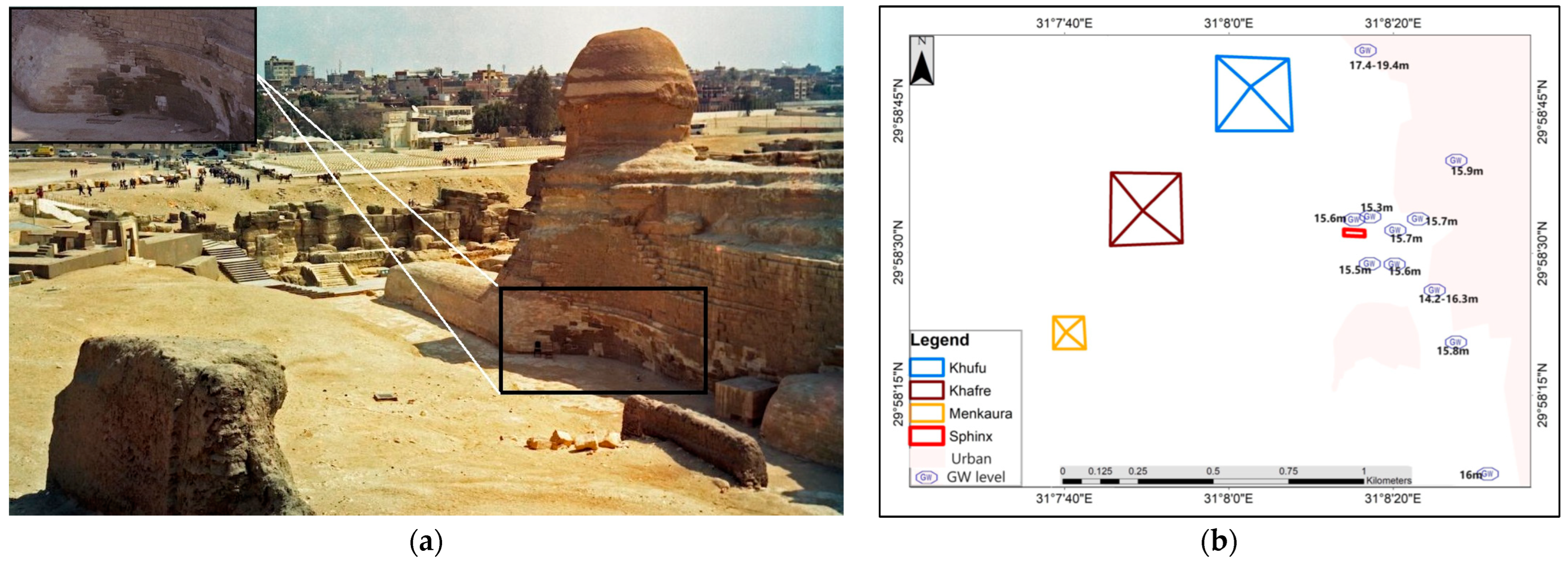
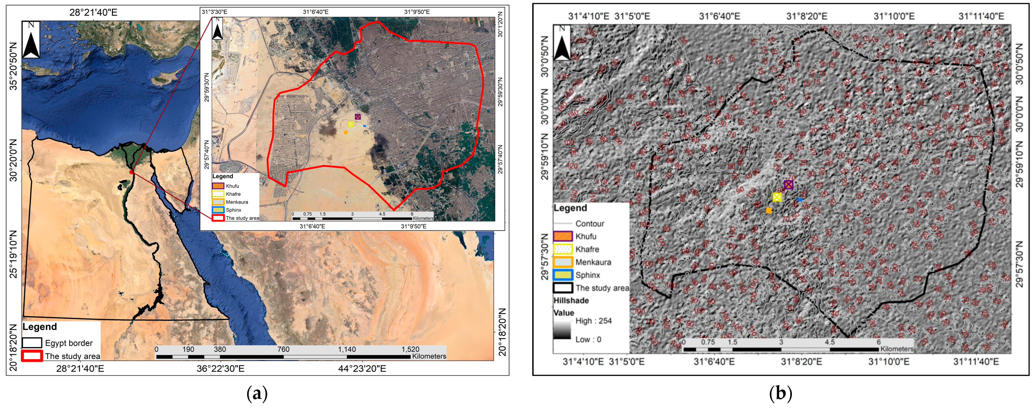
2.1. The Study Area
2.2. Material
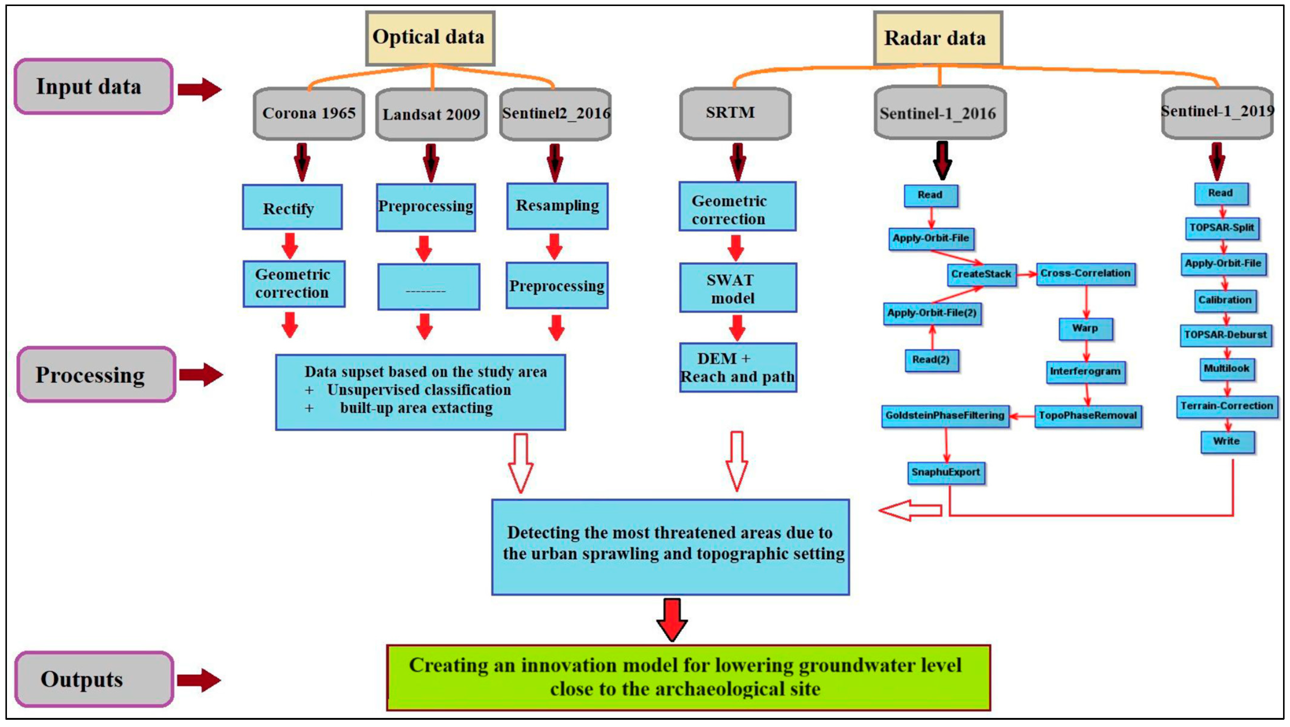
2.3. Methods
2.3.1. Optical Data Processing
2.3.2. Radar Data Processing
- Sentinel-1 (SLC) for extracting urban areas;
- Topographic setting of the study area based on the SRTM data;
- Sentinel-1 (SLC) for detecting land subsidence values;
2.3.3. Spatial Statistical Analysis
- Clusters outliers and standard distance;
- Spatial autocorrelation statistic using geographically weighted regression;
- Space-time Ripley’s K Function for Spatiotemporal Point Pattern Analysis
- Optimized Hot Spot Analysis
3. Results and Discussion
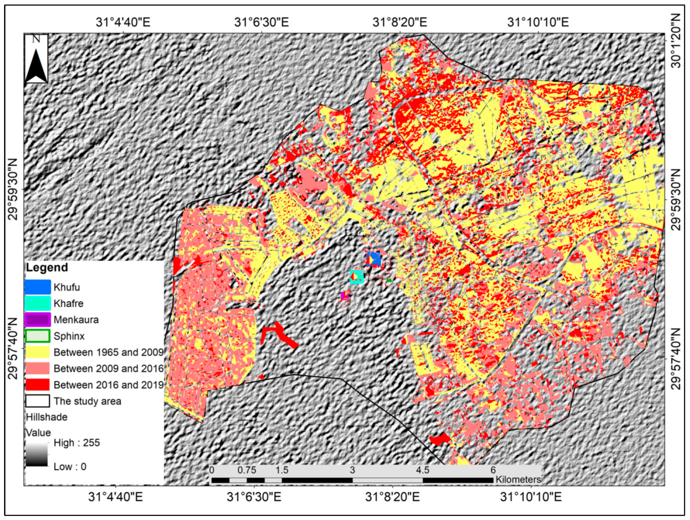
3.1. Detect the Built-Up Area Time-Series Changes
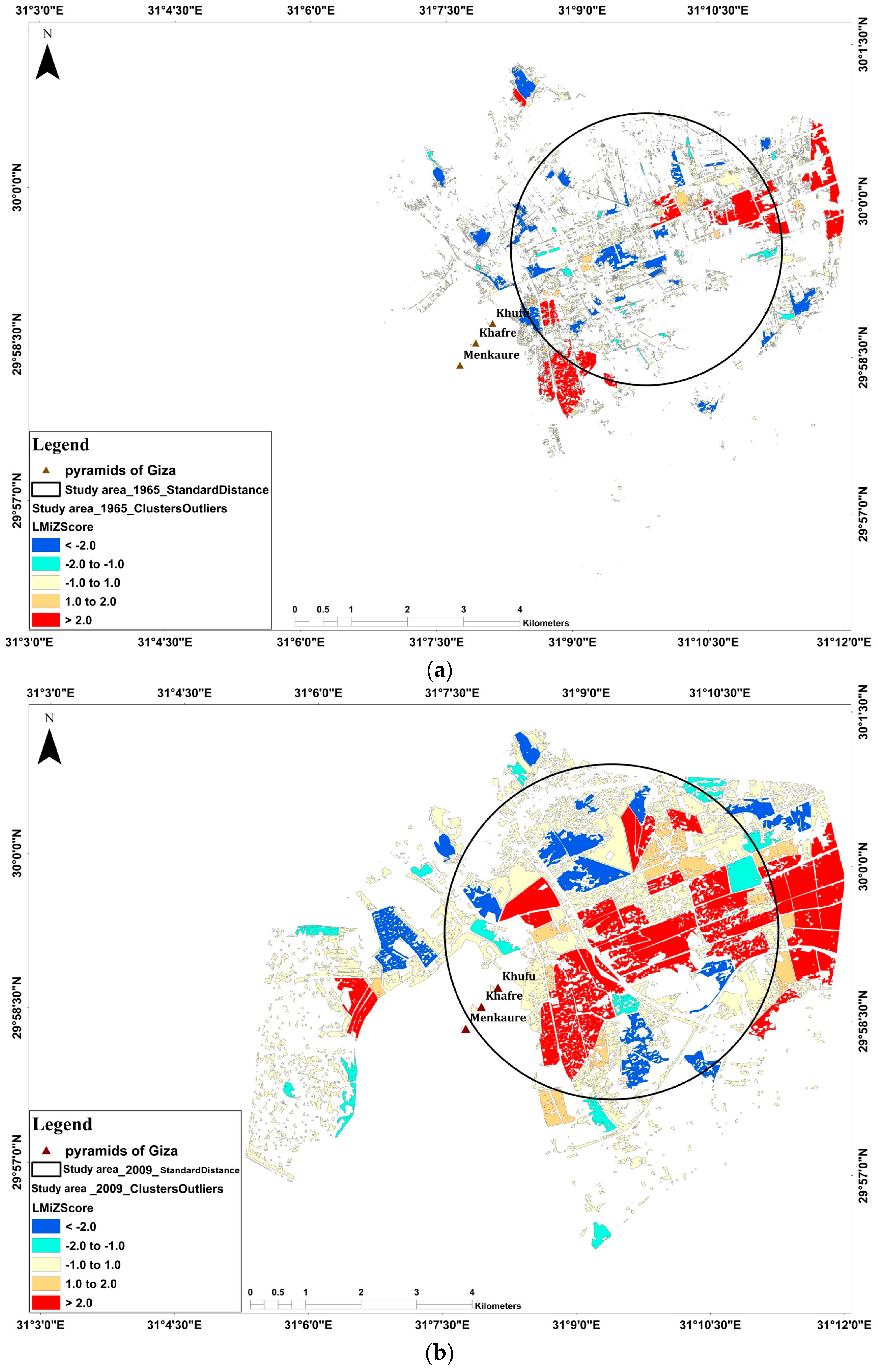
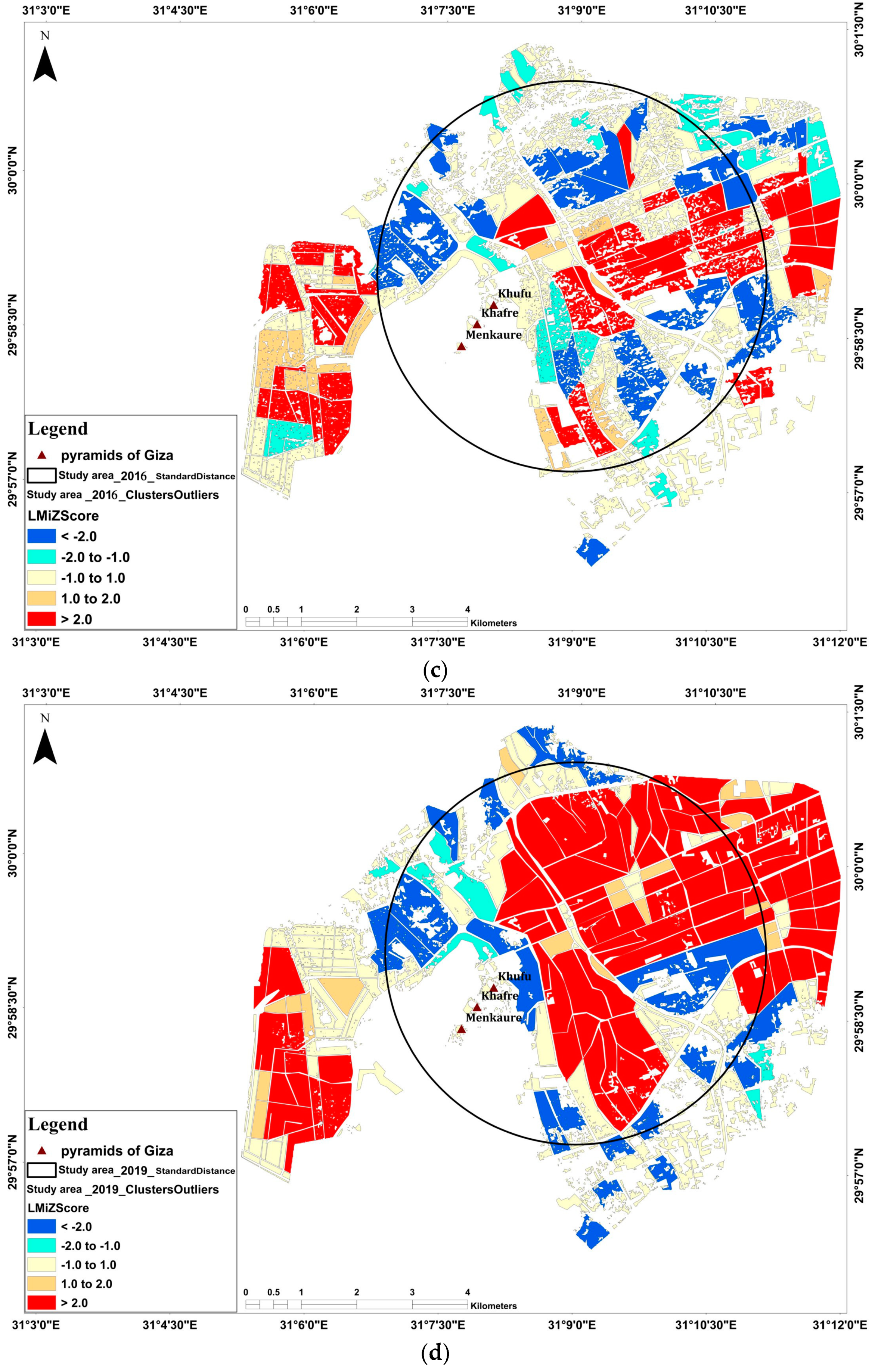
3.2. Detect the Changes by Clusters Outliers and Standard Distance
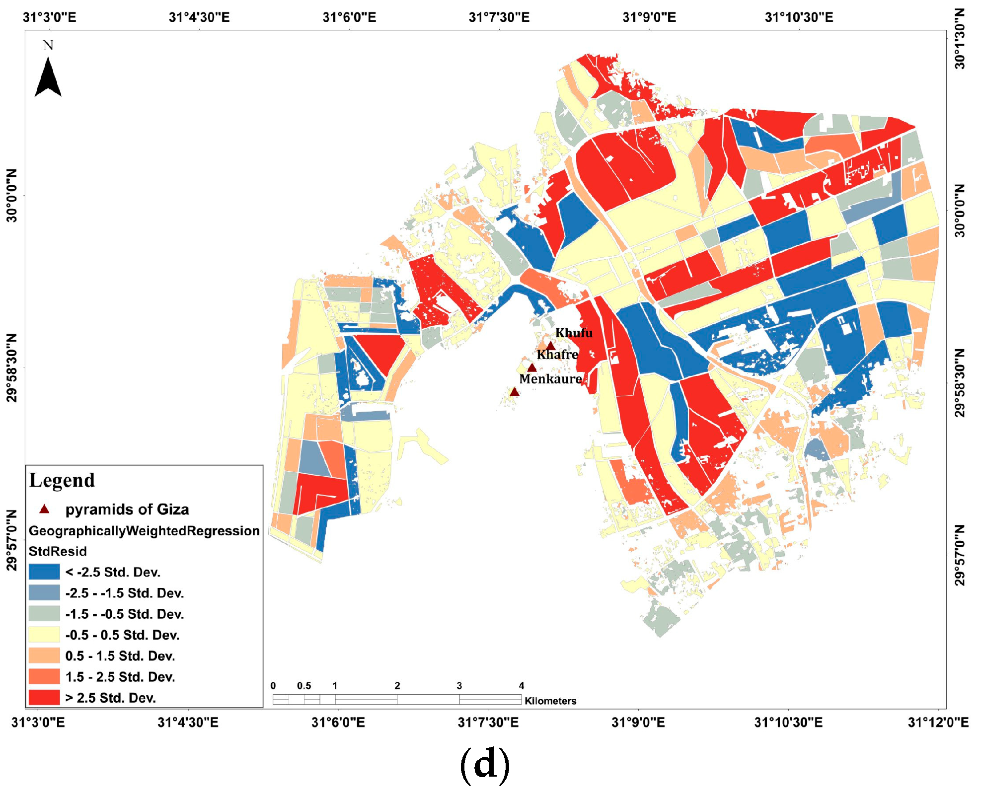
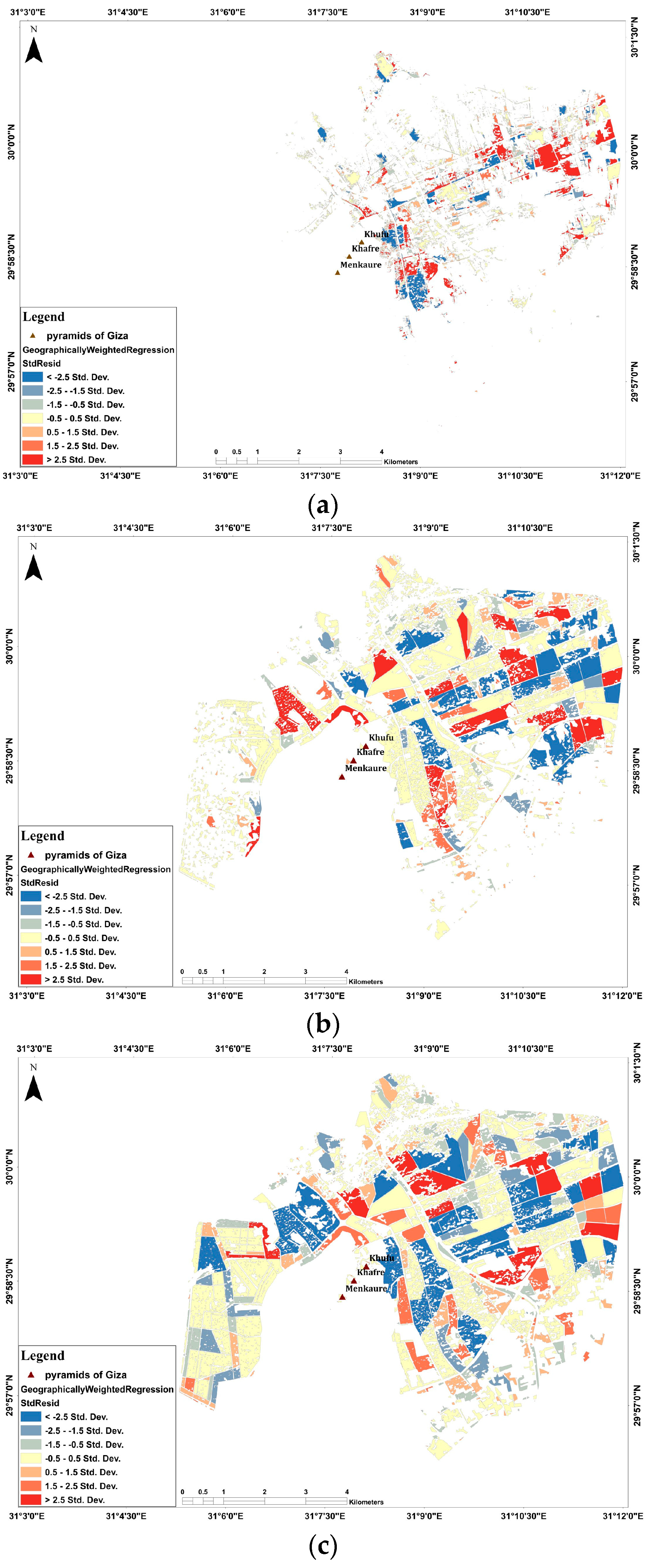
3.3. Detect the Changes by Geographically Weighted Regression
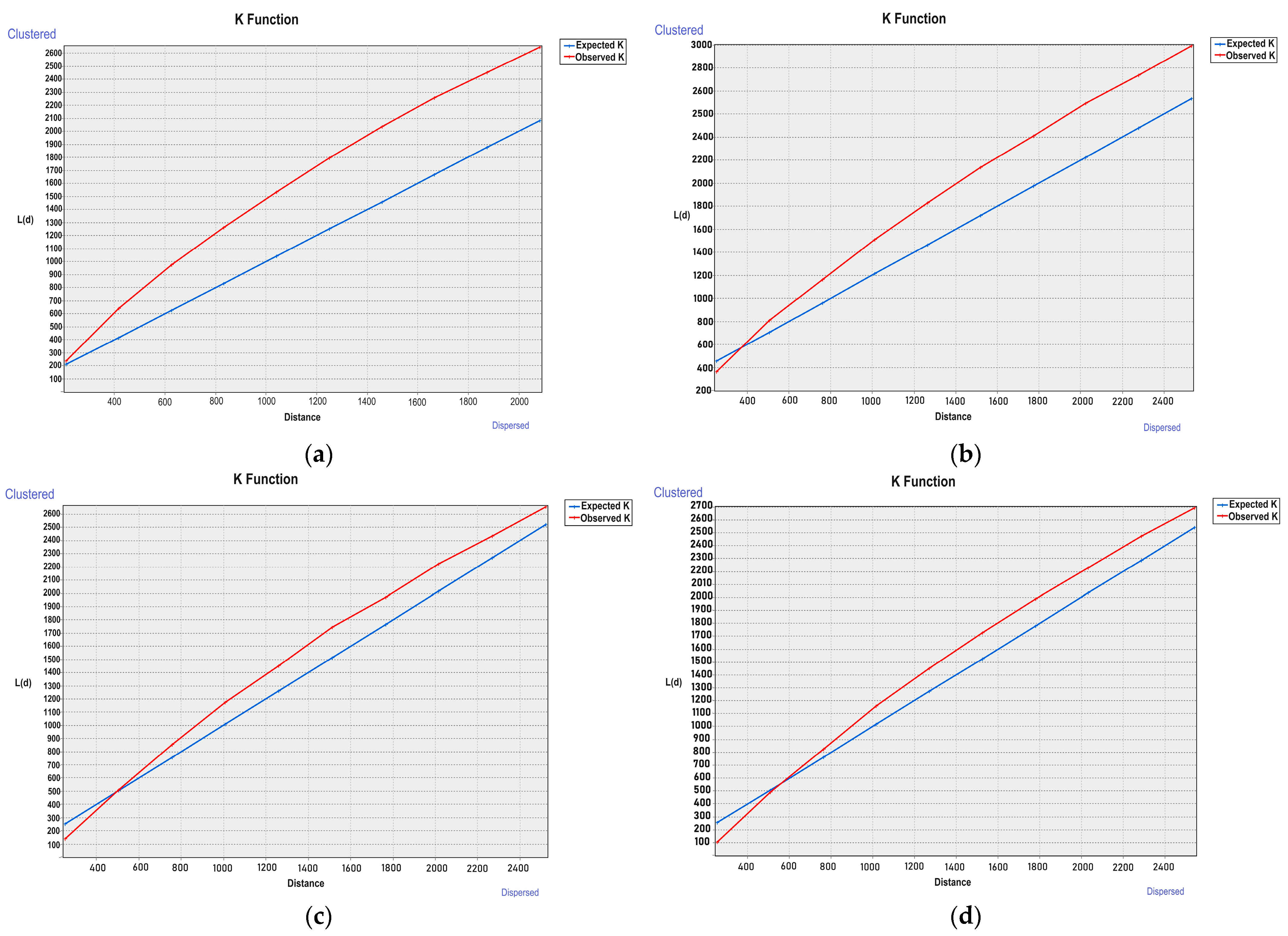
3.4. Multidistance Spatial Cluster (K Function) Time-Series Changes
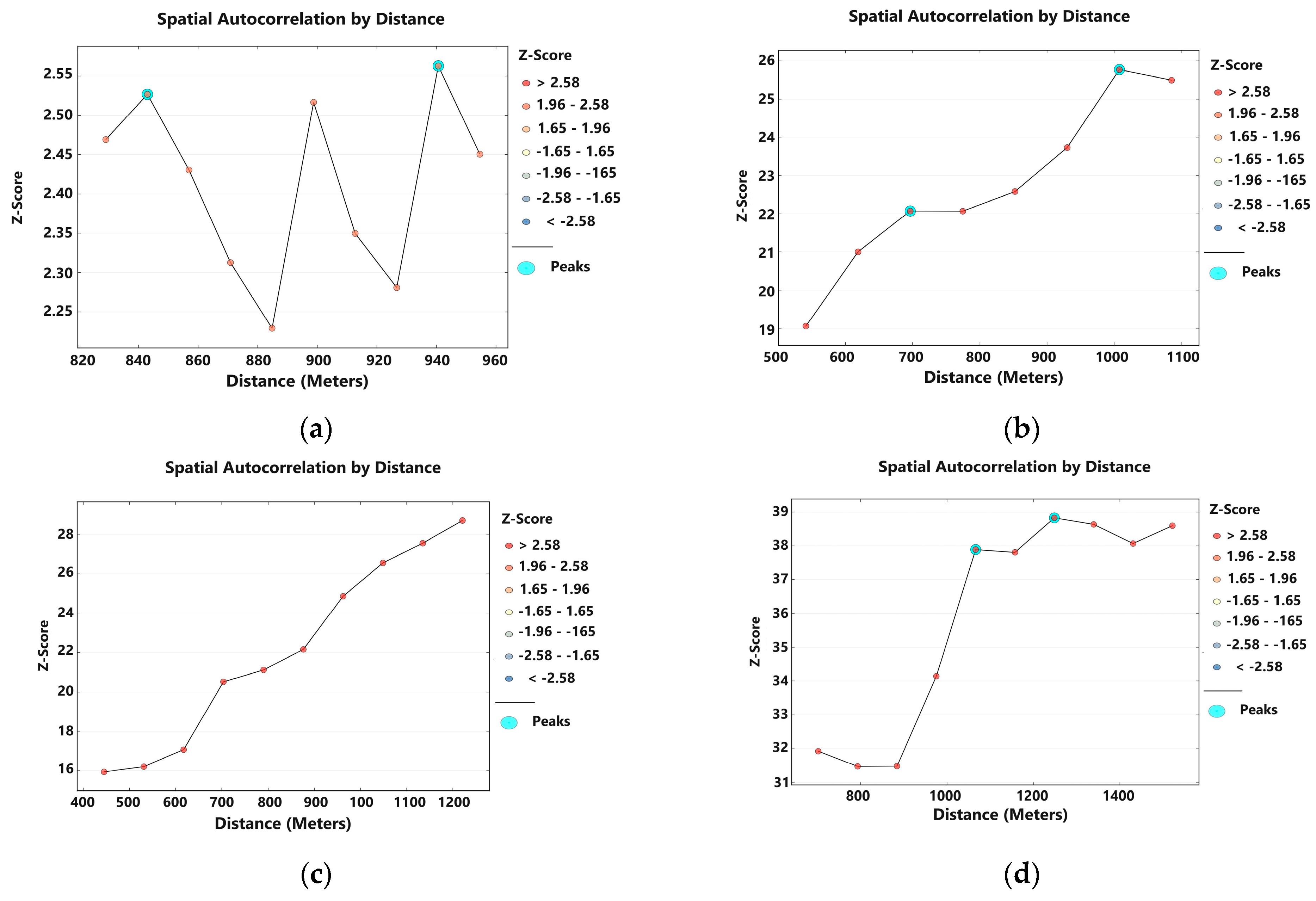
3.5. Spatial Autocorrelation Statistic Time-Series Changes
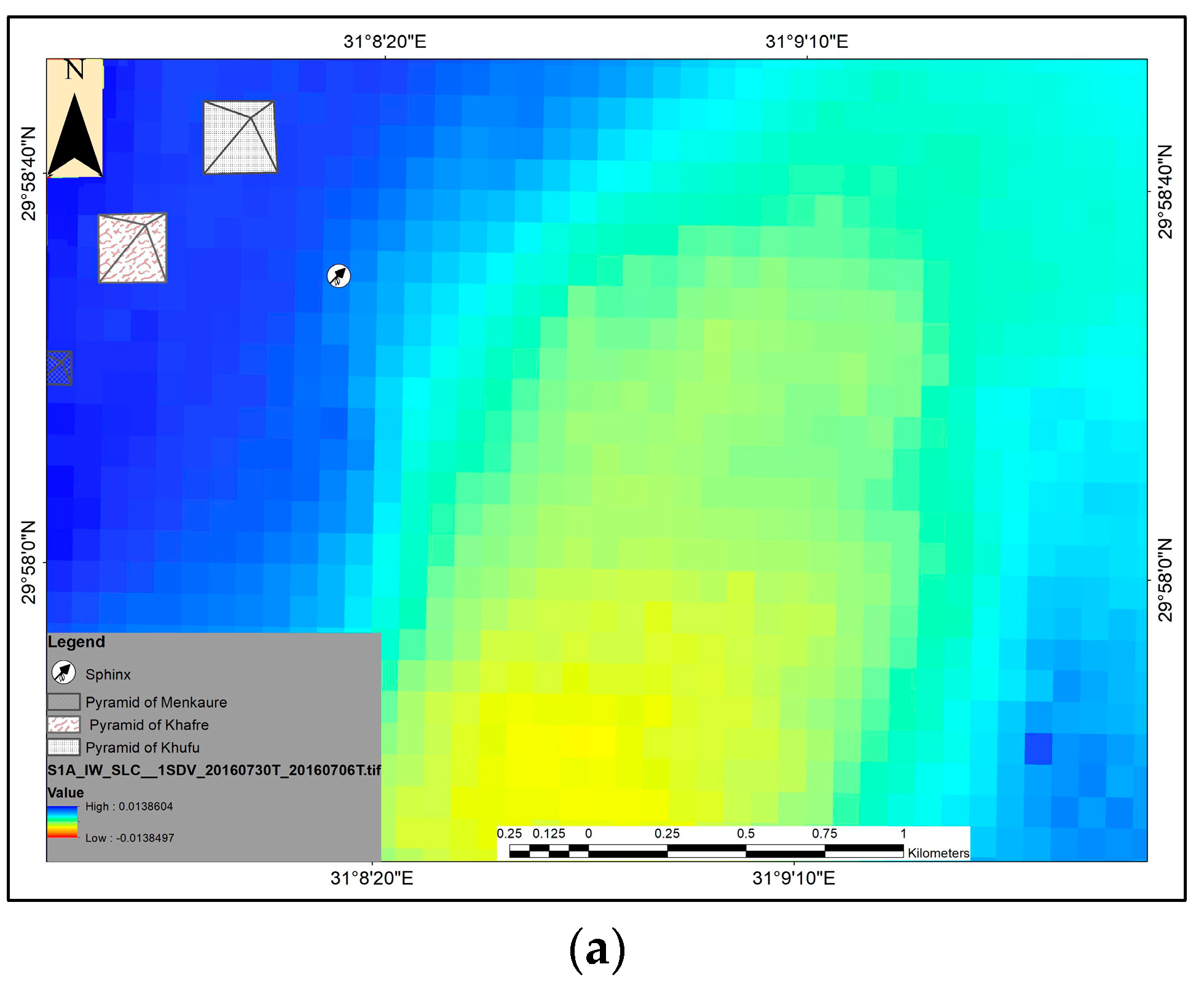
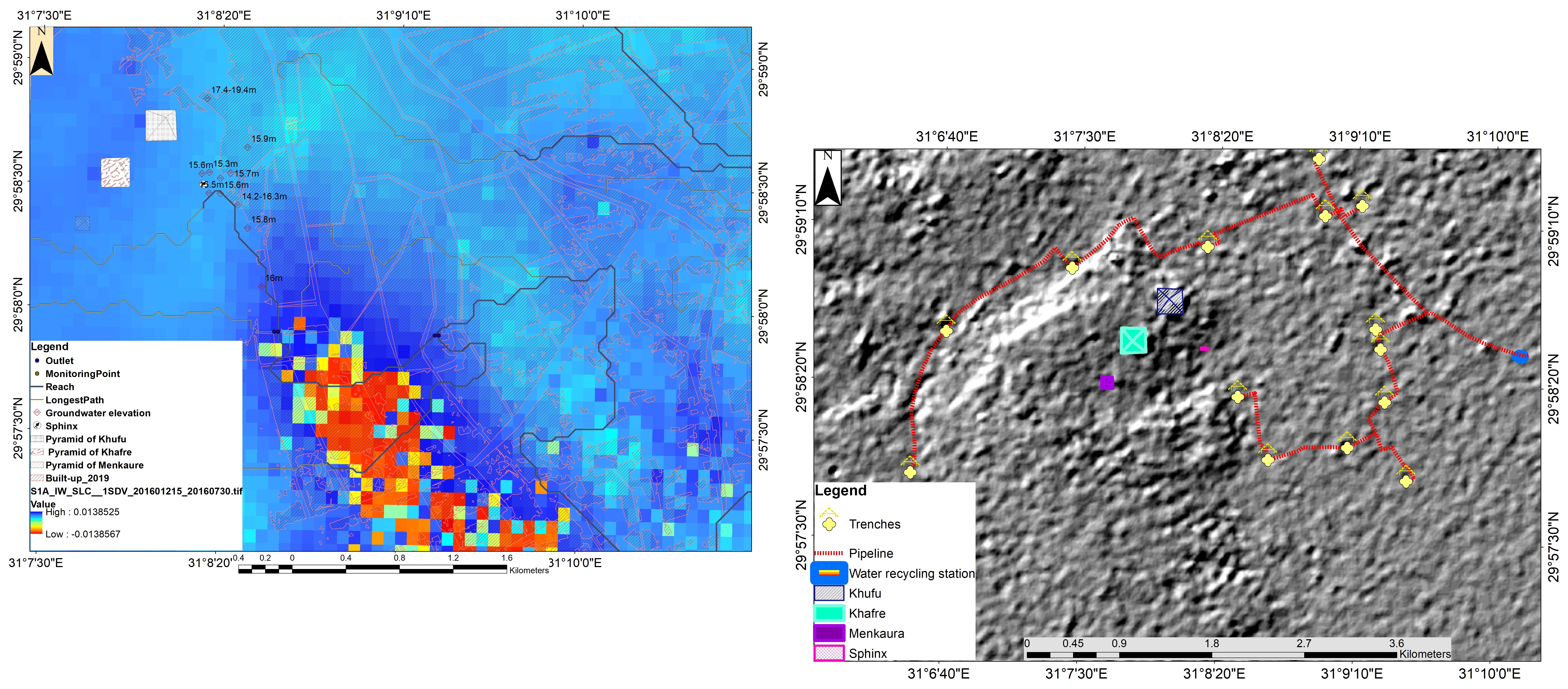
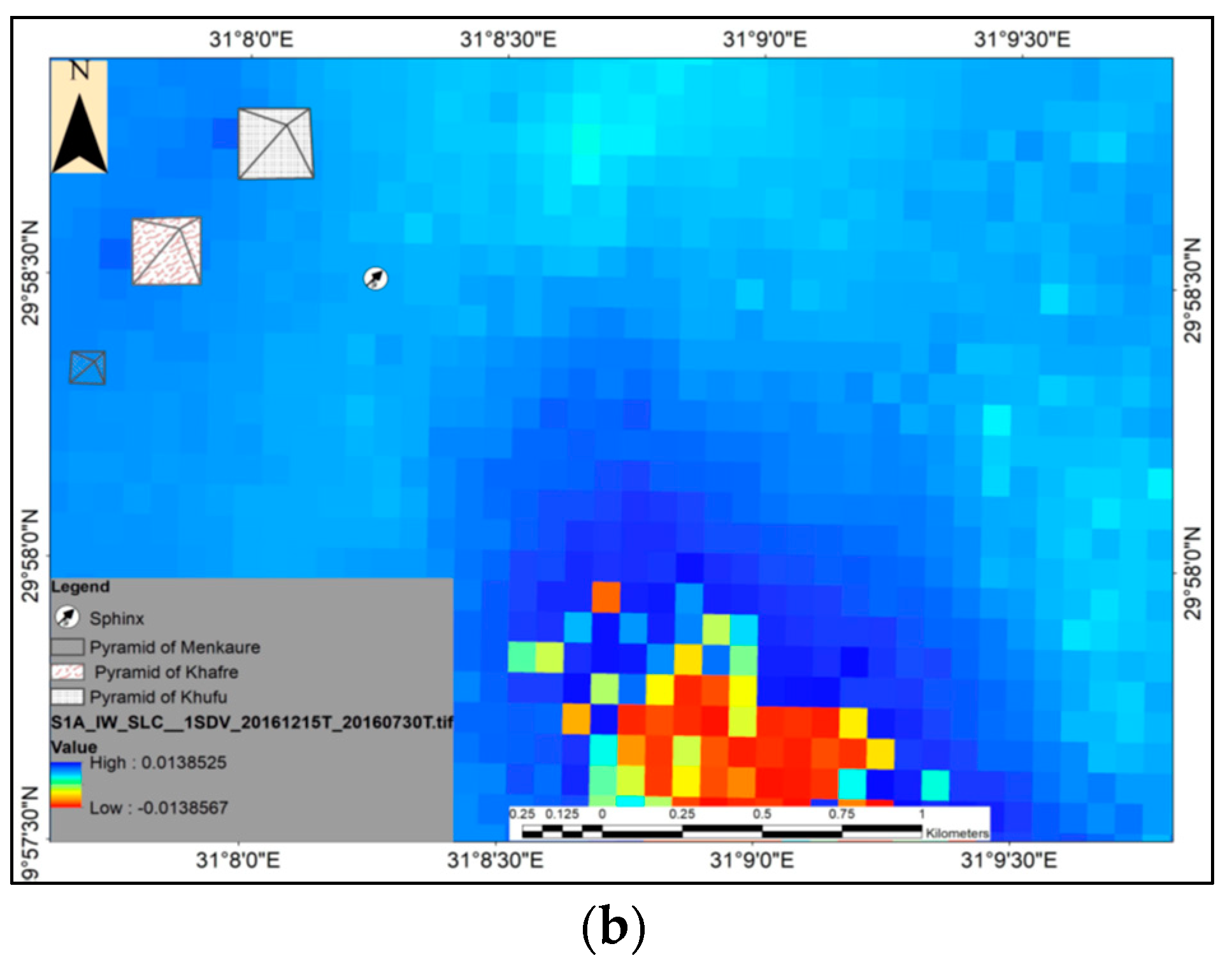
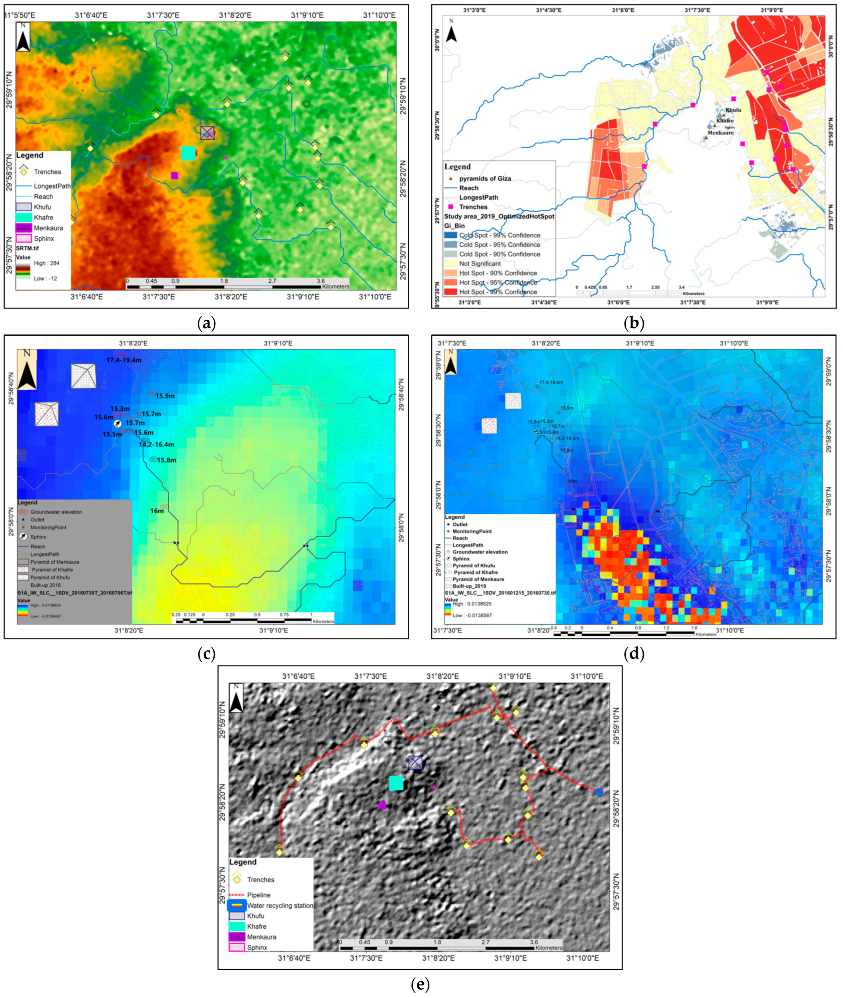
3.6. Land Subsidence (Deformation)
4. Recommendation
5. Conclusions
Author Contributions
Funding
Data Availability Statement
Acknowledgments
Conflicts of Interest
References
- Grimwade, G.; Carter, B. Managing small heritage sites with interpretation and community involvement. Int. J. Herit. Stud. 2000, 6, 33–48. [Google Scholar] [CrossRef]
- Kammeier, H.D. Managing cultural and natural heritage resources: Part I–from concepts to practice. City Time 2008, 4, 1–13. [Google Scholar]
- Bamert, M.; Ströbele, M.; Buchecker, M. Ramshackle farmhouses, useless old stables, or irreplaceable cultural heritage? Local inhabitants’ perspectives on future uses of the Walser built heritage. Land Use Policy 2016, 55, 121–129. [Google Scholar] [CrossRef]
- Ravankhah, M.; Schmidt, M. Paper 1: Developing Methodology of Disaster Risk Assessment for Cultural Heritage Sites. ANDROID Dr. Sch. Disaster Resil. 2014, 2014, 13. [Google Scholar]
- Abate, N.; Elfadaly, A.; Masini, N.; Lasaponara, R. Multitemporal 2016–2018 Sentinel-2 data enhancement for landscape archaeology: The case study of the Foggia province, Southern Italy. Remote Sens. 2020, 12, 1309. [Google Scholar] [CrossRef]
- Elfadaly, A.; Abutaleb, K.; Naguib, D.M.; Lasaponara, R. Detecting the environmental risk on the archaeological sites using satellite imagery in Basilicata Region, Italy. Egypt. J. Remote Sens. Space Sci. 2022, 25, 181–193. [Google Scholar] [CrossRef]
- Attia, W.; Ragab, D.; Abdel-Hamid, A.M.; Marghani, A.M.; Elfadaly, A.; Lasaponara, R. On the use of radar and optical satellite imagery for the monitoring of flood hazards on heritage sites in Southern Sinai, Egypt. Sustainability. 2022, 14, 5500. [Google Scholar] [CrossRef]
- Elfadaly, A.; Shams eldein, A.; Lasaponara, R. Cultural heritage management using remote sensing data and GIS techniques around the archaeological area of ancient Jeddah in Jeddah City, Saudi Arabia. Sustainability. 2019, 12, 240. [Google Scholar] [CrossRef]
- Lasaponara, R.; Elfadaly, A.; Attia, W. Low cost space technologies for operational change detection monitoring around the archaeological area of Esna-Egypt. In Computational Science and Its Applications–ICCSA 2016, Proceedings of the 16th International Conference (Proceedings, Part II 16), Beijing, China, 4–7 July 2016; Springer International Publishing: Berlin/Heidelberg, Germany, 2016; pp. 611–621. [Google Scholar]
- Badman, T.; Bomhard, B.; Fincke, A.; Langley, J.; Rosabal, P.; Sheppard, D. World Heritage in Danger. IUCN World Herit. Stud. 2009, 7. [Google Scholar]
- Mazurczyk, T.; Piekielek, N.; Tansey, E.; Goldman, B. American archives and climate change: Risks and adaptation. Clim. Risk Manag. 2018, 20, 111–125. [Google Scholar] [CrossRef]
- Holden, J.; West, L.J.; Howard, A.J.; Maxfield, E.; Panter, I.; Oxley, J. Hydrological controls of in situ preservation of waterlogged archaeological deposits. Earth-Sci. Rev. 2006, 78, 59–83. [Google Scholar] [CrossRef]
- Tassie, G.; Hassan, F. Sites and Monuments Records (SMRs) and Cultural Heritage Management. In Managing Egypt’s Cultural Heritage, Proceedings of the First Egyptian Cultural Heritage Organisation Conference on Egyptian Cultural Heritage Management; Golden House and ECHO Publications: London, UK, 2009; pp. 191–205. [Google Scholar]
- Memphis and its Necropolis—The Pyramid Fields from Giza to Dahshur. Available online: https://whc.unesco.org/en/list/86 (accessed on 8 February 2024).
- El-Bayomi, G.; Ali, R.R. Assessment of Urban Sprawl on El Minya Archeological Sites, Egypt. J. Appl. Sci. 2015, 15, 264–270. [Google Scholar] [CrossRef]
- de Noronha Vaz, E.; Cabral, P.; Caetano, M.; Nijkamp, P.; Painho, M. Urban heritage endangerment at the interface of future cities and past heritage: A spatial vulnerability assessment. Habitat Int. 2012, 36, 287–294. [Google Scholar] [CrossRef]
- Smith, M.E. Sprawl, squatters and sustainable cities: Can archaeological data shed light on modern urban issues? Camb. Archaeol. J. 2010, 20, 229–253. [Google Scholar] [CrossRef]
- Choy, D.L.; Clarke, P.; Serrao-Neumann, S.; Hales, R.; Koschade, O.; Jones, D. Coastal urban and peri-urban indigenous people’s adaptive capacity to climate change. Balanc. Urban Dev. Options Strateg. Liveable Cities 2016, 72, 441–461. [Google Scholar]
- Isendahl, C.; Smith, M.E. Sustainable agrarian urbanism: The low-density cities of the Mayas and Aztecs. Cities 2013, 31, 132–143. [Google Scholar] [CrossRef]
- Price, S.J.; Burke, H.F.; Terrington, R.L.; Reeves, H.; Boon, D.; Scheib, A.J. The 3D characterisation of the zone of human interaction and the sustainable use of underground space in urban and peri-urban environments: Case studies from the UK. Z. Der Dtsch. Ges. Geowiss. 2010, 161, 219–235. [Google Scholar] [CrossRef]
- Elfadaly, A.; Wafa, O.; Abouarab, M.A.; Guida, A.; Spanu, P.G.; Lasaponara, R. Geo-environmental estimation of land use changes and its effects on Egyptian Temples at Luxor City. ISPRS Int. J. Geo-Inf. 2017, 6, 378. [Google Scholar] [CrossRef]
- Elfadaly, A.; Lasaponara, R.; Murgante, B.; Qelichi, M.M. Cultural heritage management using analysis of satellite images and advanced GIS techniques at East Luxor, Egypt and Kangavar, Iran (a comparison case study). In Computational Science and Its Applications–ICCSA 2017, Proceedings of the 17th International Conference (Proceedings, Part IV 17), Trieste, Italy, 3–6 July 2017; Springer International Publishing: Berlin/Heidelberg, Germany, 2017; pp. 152–168. [Google Scholar]
- Satellite-Based Damage Assessment of Cultural Heritage Sites 2015. Available online: https://whc.unesco.org/en/activities/890/ (accessed on 8 February 2024).
- Santos, C.; Rapp, L. Satellite imagery, very high-resolution and processing-intensive image analysis: Potential risks under the gdpr. Air Space Law 2019, 44. [Google Scholar]
- Corrie, R.K. October. Detection of ancient Egyptian archaeological sites using satellite remote sensing and digital image processing. In Earth Resources and Environmental Remote Sensing/GIS Applications II; SPIE: Ile-de-France, France, 2011; Volume 8181, pp. 270–288. [Google Scholar]
- Maheshwari, B.; Singh, V.P.; Thoradeniya, B. Balanced Urban Development: Options and Strategies for Liveable Cities; Springer Nature: Berlin/Heidelberg, Germany, 2016; p. 601. [Google Scholar]
- Bonazza, A.; Bonora, N.; Duke, B.; Spizzichino, D.; Recchia, A.P.; Taramelli, A. Copernicus in support of monitoring, protection, and management of cultural and natural heritage. Sustainability 2022, 14, 2501. [Google Scholar] [CrossRef]
- Elfadaly, A.; Attia, W.; Qelichi, M.M.; Murgante, B.; Lasaponara, R. Management of cultural heritage sites using remote sensing indices and spatial analysis techniques. Surv. Geophys. 2018, 39, 1347–1377. [Google Scholar] [CrossRef]
- Orlando, P.; Villa, B.D. Remote sensing applications in archaeology. Archeol. E Calc. 2011, 22, 147–168. [Google Scholar]
- Lauer, D.T.; Morain, S.A.; Salomonson, V.V. The Landsat program: Its origins, evolution, and impacts. Photogramm. Eng. Remote Sens. 1997, 63, 831–838. [Google Scholar]
- Campana, S. Archaeology, remote sensing. In Encyclopedia of Geoarchaeology; Springer: Dordrecht/Berlin/Heidelberg, Germany; New York, NY, USA; London, UK, 2016; pp. 703–724. [Google Scholar]
- Cian, F.; Blasco, J.M.D.; Carrera, L. Sentinel-1 for monitoring land subsidence of coastal cities in Africa using PSInSAR: A methodology based on the integration of SNAP and staMPS. Geosciences 2019, 9, 124. [Google Scholar] [CrossRef]
- U.S. Helps Preserve base of Sphinx by Lowering Groundwater. Available online: https://eg.usembassy.gov/u-s-helps-preserve-base-sphinx-lowering-groundwater/ (accessed on 8 February 2024).
- Hemeda, S.; Sonbol, A. Sustainability problems of the Giza pyramids. Herit. Sci. 2020, 8, 1–28. [Google Scholar] [CrossRef]
- Sharafeldin, S.M.; Essa, K.S.; Youssef, M.A.; Karsli, H.; Diab, Z.E.; Sayil, N. Shallow geophysical techniques to investigate the groundwater table at the Great Pyramids of Giza, Egypt. Geosci. Instrum. Methods Data Syst. 2019, 8, 29–43. [Google Scholar] [CrossRef]
- Butzer, K.W.; Butzer, E.; Love, S. Urban geoarchaeology and environmental history at the Lost City of the Pyramids, Giza: Synthesis and review. J. Archaeol. Sci. 2013, 40, 3340–3366. [Google Scholar] [CrossRef]
- de Noronha Vaz, E.; Caetano, M.; Nijkamp, P. A multi-level spatial urban pressure analysis of the Giza pyramid plateau in Egypt. J. Herit. Tour. 2011, 6, 99–108. [Google Scholar] [CrossRef]
- Sharafeldin, M.; Essa, K.S.; Sayıl, N.; Youssef, M.A.S.; Diab, Z.E.; Karslı, H. Geophysical investigation of ground water hazards in Giza Pyramids and Sphinx using electrical resistivity tomography and ground penetrating radar: A case study. In Proceedings of the 9th Congress of the Balkan Geophysical Society, Antalya, Turkey, 5–9 November 2017; European Association of Geoscientists & Engineers: Utrecht, The Netherlands, 2017; Volume 2017, No. 1. pp. 1–5. [Google Scholar]
- A Report Published by National Geographic about the Urban Sprawling Effects on the Giza Plateau Area. Available online: https://www.nationalgeographic.com/science/article/140418-egypt-population-heritage-conservation-threats-world (accessed on 8 February 2024).
- Ancient Thebes with Its Necropolis. Available online: http://whc.unesco.org/en/soc/3597 (accessed on 8 February 2024).
- Morsy, S.W.; Halim, M.A. Reasons why the great pyramids of Giza remain the only surviving wonder of the ancient world: Drawing ideas from the structure of the Giza pyramids to nuclear power plants. J. Civ. Eng. Archit. 2015, 9, 1191–1201. [Google Scholar]
- Nell, E.; Ruggles, C. The orientations of the Giza pyramids and associated structures. J. Hist. Astron. 2014, 45, 304–360. [Google Scholar] [CrossRef]
- Der Manuelian, P. Giza 3D: Digital archaeology and scholarly access to the Giza pyramids: The Giza project at Harvard university. In 2013 Digital Heritage International Congress (DigitalHeritage); IEEE: New York, NY, USA, 2013; Volume 2, pp. 727–734. [Google Scholar]
- Magli, G. The Giza ‘written’ landscape and the double project of King Khufu. Time Mind 2016, 9, 57–74. [Google Scholar] [CrossRef]
- USGS. Available online: https://earthexplorer.usgs.gov/ (accessed on 8 February 2024).
- ArcSWAT. Available online: https://swat.tamu.edu/software/arcswat/ (accessed on 8 February 2024).
- The Copernicus Data Space Ecosystem. Available online: https://dataspace.copernicus.eu/ (accessed on 8 February 2024).
- Duan, W.; Zhang, H.; Wang, C.; Tang, Y. Multi-temporal InSAR parallel processing for Sentinel-1 large-scale surface deformation mapping. Remote Sens. 2020, 12, 3749. [Google Scholar] [CrossRef]
- Richards, M.A. A Beginner’s Guide to interferometric SAR concepts and signal processing [AESS tutorial IV]. IEEE Aerosp. Electron. Syst. Mag. 2007, 22, 5–29. [Google Scholar] [CrossRef]
- Vrînceanu, C.A.; Grebby, S.; Marsh, S. The performance of speckle filters on Copernicus Sentinel-1 SAR images containing natural oil slicks. Q. J. Eng. Geol. Hydrogeol. 2023, 56, qjegh2022-046. [Google Scholar] [CrossRef]
- How to Radiometrically Terrain-Correct (RTC) Sentinel-1 Data Using GAMMA Software. Available online: https://asf.alaska.edu/how-to/data-recipes/how-to-radiometrically-terrain-correct-rtc-sentinel-1-data-using-gamma-software/ (accessed on 8 February 2024).
- Semenzato, A.; Pappalardo, S.E.; Codato, D.; Trivelloni, U.; De Zorzi, S.; Ferrari, S.; De Marchi, M.; Massironi, M. Mapping and monitoring urban environment through sentinel-1 SAR data: A case study in the Veneto region (Italy). ISPRS Int. J. Geo-Inf. 2020, 9, 375. [Google Scholar] [CrossRef]
- Koltsida, E.; Kallioras, A. Multi-Variable SWAT Model Calibration Using Satellite-Based Evapotranspiration Data and Streamflow. Hydrology 2022, 9, 112. [Google Scholar] [CrossRef]
- Al-Khafaji, M.S.; Al-Sweiti, F.H. Integrated impact of digital elevation model and land cover resolutions on simulated runoff by SWAT Model. Hydrol. Earth Syst. Sci. Discuss. 2017, 1–26. [Google Scholar] [CrossRef]
- Lin, S.; Jing, C.; Chaplot, V.; Yu, X.; Zhang, Z.; Moore, N.; Wu, J. Effect of DEM resolution on SWAT outputs of runoff, sediment and nutrients. Hydrol. Earth Syst. Sci. Discuss. 2010, 7, 4411–4435. [Google Scholar]
- Winchell, M.; Srinivasan, R.; Di Luzio, M.; Arnold, J. ArcSWAT Interface for SWAT2012: User’s Guide; Blackland Research Center, Texas AgriLife Research, College Station: Temple, TX, USA, 2013; pp. 1–464. [Google Scholar]
- Tan, M.L.; Ficklin, D.L.; Dixon, B.; Yusop, Z.; Chaplot, V. Impacts of DEM resolution, source, and resampling technique on SWAT-simulated streamflow. Appl. Geogr. 2015, 63, 357–368. [Google Scholar] [CrossRef]
- Zhang, Y.; Wu, H.; Li, M.; Kang, Y.; Lu, Z. Investigating ground subsidence and the causes over the whole Jiangsu Province, China using sentinel-1 SAR data. Remote Sens. 2021, 13, 179. [Google Scholar] [CrossRef]
- Rateb, A.; Abotalib, A.Z. Inferencing the land subsidence in the Nile Delta using Sentinel-1 satellites and GPS between 2015 and 2019. Sci. Total Environ. 2020, 729, 138868. [Google Scholar] [CrossRef] [PubMed]
- Hu, L.; Dai, K.; Xing, C.; Li, Z.; Tomás, R.; Clark, B.; Shi, X.; Chen, M.; Zhang, R.; Qiu, Q.; et al. Land subsidence in Beijing and its relationship with geological faults revealed by Sentinel-1 InSAR observations. Int. J. Appl. Earth Obs. Geoinf. 2019, 82, 101886. [Google Scholar] [CrossRef]
- Sánchez-Martín, J.M.; Rengifo-Gallego, J.I.; Blas-Morato, R. Hot spot analysis versus cluster and outlier analysis: An enquiry into the grouping of rural accommodation in Extremadura (Spain). ISPRS Int. J. Geo-Inf. 2019, 8, 176. [Google Scholar] [CrossRef]
- Martin, C.; Stewart, F. Geographically Weighted Regression: A Tutorial on Using GWR in ArcGIS 9.3; National Centre for Geocomputation, National University of Ireland: Maynooth, Ireland, 2009; pp. 1–27. [Google Scholar]
- Fotheringham, A.S.; Brunsdon, C.; Charlton, M. Geographically Weighted Regression: The Analysis of Spatially Varying Relationships; John Wiley & Sons: Hoboken, NJ, USA, 2003. [Google Scholar]
- Brunsdon, C.; Fotheringham, A.S.; Charlton, M.E. Geographically weighted regression: A method for exploring spatial nonstationarity. Geogr. Anal. 1996, 28, 281–298. [Google Scholar] [CrossRef]
- Lu, B.; Charlton, M.; Harris, P.; Fotheringham, A.S. Geographically weighted regression with a non-Euclidean distance metric: A case study using hedonic house price data. Int. J. Geogr. Inf. Sci. 2014, 28, 660–681. [Google Scholar] [CrossRef]
- Dubé, J.; Legros, D. Spatial autocorrelation. In Spatial Econometrics Using Microdata; Springer: Berlin/Heidelberg, Germany, 2014; pp. 59–91. [Google Scholar] [CrossRef]
- Wang, Y.; Gui, Z.; Wu, H.; Peng, D.; Wu, J.; Cui, Z. Optimizing and accelerating space–time Ripley’s K function based on Apache Spark for distributed spatiotemporal point pattern analysis. Future Gener. Comput. Syst. 2020, 105, 96–118. [Google Scholar] [CrossRef]
- Getis, A.; Ord, J.K. The analysis of spatial association by use of distance statistics. Geogr. Anal. 1992, 24, 189–206. [Google Scholar] [CrossRef]
- Getis, A. Local spatial statistics: An overview. In Spatial Analysis: Modelling in a GIS Environment; John Wiley & Sons: Hoboken, NJ, USA, 1996; pp. 261–277. [Google Scholar]
- Ord, J.K.; Getis, A. Local spatial autocorrelation statistics: Distributional issues and an application. Geogr. Anal. 1995, 27, 286–306. [Google Scholar] [CrossRef]
- Casarotto, A.; Pelgrom, J.; Stek, T.D. Testing settlement models in the early Roman colonial landscapes of Venusia (291 BC), Cosa (273 BC) and Aesernia (263 BC). J. Field Archaeol. 2016, 41, 568–586. [Google Scholar] [CrossRef]
- Casarotto, A. Spatial Patterns in Landscape Archaeology: A GIS Procedure to Study Settlement Organization in Early Roman Colonial Territories; Leiden University Press: Leiden, The Netherlands, 2018. [Google Scholar]
- Bokhari, R.; Shu, H.; Tariq, A.; Al-Ansari, N.; Guluzade, R.; Chen, T.; Jamil, A.; Aslam, M. Land subsidence analysis using synthetic aperture radar data. Heliyon 2023, 9, e14690. [Google Scholar] [CrossRef]
- Ghazifard, A.; Akbari, E.; Shirani, K.; Safaei, H. Evaluating land subsidence by field survey and D-InSAR technique in Damaneh City, Iran. J. Arid. Land 2017, 9, 778–789. [Google Scholar] [CrossRef]
- Tiwari, R.K.; Malik, K.; Arora, M.K. Urban subsidence detection using the sentinel-1 multi-temporal INSAR data. In Proceedings of the 38th Asian Conference on Remote Sensing-Space Applications: Touching Human Lives, New Delhi, India, 23–27 October 2017; ACRS: Seattle, WA, USA, 2017; Volume 27, pp. 2410–2414. [Google Scholar]
- Bhattarai, R.; Alifu, H.; Maitiniyazi, A.; Kondoh, A. Detection of land subsidence in Kathmandu Valley, Nepal, using DInSAR technique. Land 2017, 6, 39. [Google Scholar] [CrossRef]
- Nalakurthi, N.S.R.N.; Behera, M.R. Detection of Land Subsidence using Sentinel-1 Interferometer andIts Relationship withSea-Level-Rise, Groundwater, andInundation: A Case Study along Mumbai Coastal City. 2022. Available online: https://www.researchsquare.com/article/rs-1392714/v1 (accessed on 8 February 2024).
- Holtorf, C.; Ortman, O. Endangerment and conservation ethos in natural and cultural heritage: The case of zoos and archaeological sites. Int. J. Herit. Stud. 2008, 14, 74–90. [Google Scholar] [CrossRef]
- Elfadaly, A.; Attia, W.; Lasaponara, R. Monitoring the environmental risks around Medinet Habu and Ramesseum Temple at West Luxor, Egypt, using remote sensing and GIS techniques. J. Archaeol. Method Theory 2018, 25, 587–610. [Google Scholar] [CrossRef]
- Elfadaly, A.; Murgante, B.; Qelichi, M.M.; Lasaponara, R.; Hosseini, A. A comparative analysis of temporal changes in urban land use resorting to advanced remote sensing and GIS in Karaj, Iran and Luxor, Egypt. In Computational Science and Its Applications–ICCSA 2019, Proceedings of the 19th International Conference (Proceedings, Part V 19), Saint Petersburg, Russia, 1–4 July 2019; Springer International Publishing: Berlin/Heidelberg, Germany, 2019; pp. 689–703. [Google Scholar]
- Engeman, R.M.; Couturier, K.J.; Felix, R.K.; Avery, M.L. Feral swine disturbance at important archaeological sites. Environ. Sci. Pollut. Res. 2013, 20, 4093–4098. [Google Scholar] [CrossRef] [PubMed]
- Louiset, T.; Pamart, A.; Gattet, E.; Raharijaona, T.; De Luca, L.; Ruffier, F. A shape-adjusted tridimensional reconstruction of cultural heritage artifacts using a miniature quadrotor. Remote Sens. 2016, 8, 858. [Google Scholar] [CrossRef]
- Balla, A.; Pavlogeorgatos, G.; Tsiafakis, D.; Pavlidis, G. Recent advances in archaeological predictive modeling for archeological research and cultural heritage management. Mediterr. Archaeol. Archaeom. 2014, 14, 143–144. [Google Scholar]
- Elfadaly, A.; Lasaponara, R. On the use of satellite imagery and GIS tools to detect and characterize the urbanization around heritage sites: The case studies of the Catacombs of Mustafa Kamel in Alexandria, Egypt and the Aragonese Castle in Baia, Italy. Sustainability 2019, 11, 2110. [Google Scholar] [CrossRef]
- Lasaponara, R.; Murgante, B.; Elfadaly, A.; Qelichi, M.M.; Shahraki, S.Z.; Wafa, O.; Attia, W. Spatial open data for monitoring risks and preserving archaeological areas and landscape: Case studies at Kom el Shoqafa, Egypt and Shush, Iran. Sustainability 2017, 9, 572. [Google Scholar] [CrossRef]


| Number | Satellite | Sensor | Acquisition Date | Source |
|---|---|---|---|---|
| 1 | Corona | KH-4A | 25 January 1965 | USGS |
| 2 | Landsat5 | TM | 7 May 2009 | USGS |
| 3 | Sentinel | 2A | 25 December 2016 | USGS |
| 4 | SRTM | 1 arc-second | 22 September 2014 | USGS |
| 5 | Sentinel | 1A_IW_SLC | 6 and 30 July, and 15 December 2016 | ESA |
| 6 | Sentinel | 1A_IW_SLC | 3 July 2019 | ESA |
| Year | Urban Mass (km2) | Change Detection ± (km2) |
|---|---|---|
| 1965 | 5083 | 16,715 |
| 2009 | 21,798 | 9289 |
| 2016 | 31,087 | 8695 |
| 2019 | 39,782 | - |
| Distance (m) | Moran’s Index | z-Score |
|---|---|---|
| 829.00 | 0.000859 | 2.468979 |
| 842.95 | 0.000868 | 2.526718 |
| 856.91 | 0.000820 | 2.430553 |
| 870.86 | 0.000767 | 2.312585 |
| 884.81 | 0.000723 | 2.229052 |
| 898.77 | 0.000796 | 2.516628 |
| 912.72 | 0.000729 | 2.349612 |
| 926.67 | 0.000697 | 2.280936 |
| 940.63 | 0.000780 | 2.562688 |
| 954.58 | 0.000734 | 2.450355 |
| Distance (m) | Moran’s Index | z-Score |
|---|---|---|
| 541.00 | 0.114091 | 19.059431 |
| 618.80 | 0.110322 | 21.001711 |
| 696.61 | 0.102889 | 22.071586 |
| 774.41 | 0.092411 | 22.068745 |
| 852.21 | 0.085496 | 22.583187 |
| 930.01 | 0.082103 | 23.730188 |
| 1007.82 | 0.082640 | 25.771371 |
| 1085.62 | 0.076208 | 25.492819 |
| Distance (m) | Moran’s Index | z-Score |
|---|---|---|
| 445.00 | 0.150765 | 15.941361 |
| 531.22 | 0.125013 | 16.208135 |
| 617.44 | 0.112533 | 17.062234 |
| 703.66 | 0.118415 | 20.513646 |
| 789.88 | 0.109149 | 21.116408 |
| 876.10 | 0.103648 | 22.154363 |
| 962.32 | 0.106204 | 24.861730 |
| 1048.54 | 0.104824 | 26.548377 |
| 1134.76 | 0.100804 | 27.544697 |
| 1220.98 | 0.097990 | 28.696645 |
| Distance (m) | Moran’s Index | z-Score |
|---|---|---|
| 702.00 | 0.216568 | 31.928737 |
| 793.07 | 0.188440 | 31.472736 |
| 884.14 | 0.167797 | 31.479186 |
| 975.21 | 0.166038 | 34.136998 |
| 1066.28 | 0.169543 | 37.894397 |
| 1157.34 | 0.156790 | 37.813164 |
| 1248.41 | 0.150946 | 38.830281 |
| 1339.48 | 0.140816 | 38.636843 |
| 1430.55 | 0.130735 | 38.070068 |
| 1521.62 | 0.125271 | 38.597769 |
Disclaimer/Publisher’s Note: The statements, opinions and data contained in all publications are solely those of the individual author(s) and contributor(s) and not of MDPI and/or the editor(s). MDPI and/or the editor(s) disclaim responsibility for any injury to people or property resulting from any ideas, methods, instructions or products referred to in the content. |
© 2024 by the authors. Licensee MDPI, Basel, Switzerland. This article is an open access article distributed under the terms and conditions of the Creative Commons Attribution (CC BY) license (https://creativecommons.org/licenses/by/4.0/).
Share and Cite
Elfadaly, A.; Zanaty, N.; Mostafa, W.; Hendawy, E.; Lasaponara, R. Multi-Sensor Satellite Images for Detecting the Effects of Land-Use Changes on the Archaeological Area of Giza Necropolis, Egypt. Land 2024, 13, 471. https://doi.org/10.3390/land13040471
Elfadaly A, Zanaty N, Mostafa W, Hendawy E, Lasaponara R. Multi-Sensor Satellite Images for Detecting the Effects of Land-Use Changes on the Archaeological Area of Giza Necropolis, Egypt. Land. 2024; 13(4):471. https://doi.org/10.3390/land13040471
Chicago/Turabian StyleElfadaly, Abdelaziz, Naglaa Zanaty, Wael Mostafa, Ehab Hendawy, and Rosa Lasaponara. 2024. "Multi-Sensor Satellite Images for Detecting the Effects of Land-Use Changes on the Archaeological Area of Giza Necropolis, Egypt" Land 13, no. 4: 471. https://doi.org/10.3390/land13040471
APA StyleElfadaly, A., Zanaty, N., Mostafa, W., Hendawy, E., & Lasaponara, R. (2024). Multi-Sensor Satellite Images for Detecting the Effects of Land-Use Changes on the Archaeological Area of Giza Necropolis, Egypt. Land, 13(4), 471. https://doi.org/10.3390/land13040471