Abstract
Habitat modification due to human activities threatens species survival. While some species can inhabit habitat patches in anthropogenic landscapes, their occurrence often depends on landscape structure. We assessed the effects of landscape structure on brown howler monkey (Alouatta guariba clamitans) occurrence in an urban scenario. We conducted censuses in 59 forest patches from 2014 to 2016 in Rio Grande do Sul State, Brazil. We evaluated patch occurrence (presence/absence) in response to landscape composition (forest cover, arboreal crops, urban areas, open areas, and water) and configuration (patch density), considering the scale of effect. Water, urban, and open areas were the most important predictors of howler presence. Their presence was notably higher in landscapes with more water, likely because these landscapes consist of rural areas with low urbanization, less farming, and relatively high forest cover. Presence of howlers was positively associated with forest cover and negatively related to urban areas, open areas, and arboreal crops. Resource scarcity and increased mortality risks from human pressures, such as domestic dog attacks, electrocution, and roadkill on these land covers may explain these relationships. We highlight the importance of conserving and increasing forest cover in anthropogenic landscapes to protect species reliant on forested habitats, like howler monkeys.
1. Introduction
Human population growth and urban expansion are among the main drivers of land-use change worldwide [1]. Habitat modification caused by humans pushes species to live in habitat patches surrounded by a matrix composed of land covers such as human settlements, roads, or agricultural fields [1,2,3]. Species persistence in human-modified landscapes are likely to depend highly on landscape structure (i.e., landscape composition—the types or amounts of different land covers in the landscape, and configuration—the spatial arrangement of the land covers in the landscape) [4,5,6,7]. Yet, our knowledge of how landscape structure mediates the occurrence of most species in anthropogenic landscapes is still poor. Additionally, most studies assessing the effects of landscape structure focus on the effects of landscape changes in natural habitats [8,9], particularly habitat loss and fragmentation [10], giving minor attention to the effects that other land covers can have on species. Understanding which landscape attributes favor or threaten species occurrence in anthropogenic landscapes is key to optimizing the design of strategies for species conservation [11].
Habitat loss is widely considered the major factor leading to species loss across most taxa [10,12]. Habitat loss reduces resource availability and landscape connectivity [13] and increases disease risk [14], competition [15], and/or stress [16]. The effects of habitat fragmentation on species, however, are still debated [17,18]. This is mainly due to differing conceptualizations of habitat fragmentation (i.e., fragmentation measured as part of habitat loss or independent of habitat loss; see [10]), which lead to different methods to measure it (e.g., using a patch scale vs. landscape scale). Studies conceiving fragmentation as part of habitat loss typically measure fragmentation using patch-scale variables (e.g., patch size or patch isolation) and generally infer that increasing fragmentation has strong negative effects on species [18,19,20]. Yet, many researchers in landscape ecology argue that it is important to determine the effects of fragmentation independent of the effects of habitat amount (i.e., fragmentation per se [10,21,22,23]). Assessing the independent effects of habitat fragmentation is possible by controlling for the effects of habitat amount at the landscape scale, either statistically or experimentally [10]. From this perspective, fragmentation effects need to be assessed at the landscape scale and are found to be mainly weak on species [24,25]. The lack of negative effects of fragmentation per se on species at the landscape scale is likely because the higher the number of patches in the landscape, the lower the mean nearest patch distance [10,24], which increases between-patch movement success and, therefore, resource availability [24].
Other landscape attributes, such as matrix composition (i.e., the type or the amount of land covers that are not original habitat for a particular species in the landscape), may also affect the occurrence of species in anthropogenic landscapes. The perception of the landscape matrix by scientists has progressively changed from an inhospitable area to a heterogeneous mosaic of different land covers [26,27,28]. Depending on the land cover, the matrix might facilitate or impede species dispersal, reproduction, or nutrition [26,29,30]. The difference in matrix effects appears to depend largely on the similarity/dissimilarity of each matrix land cover to the primary habitat of the studied species (i.e., low- or high-quality matrix) [31,32,33]. For instance, for species with arboreal locomotion, a high-quality matrix dominated by arboreal land covers, such as arboreal crops, offers higher dispersal, reproduction, or feeding opportunities [26]. Conversely, a low-quality matrix may not provide food resources or refuge, and may increase the risk of death from increased exposure to humans, predators, roadkill, or electrocution [34,35,36,37].
Primates are widespread in most megadiverse regions of the world, where they live in a variety of ecosystems, including highly human-modified ecosystems immersed in peri-urban and urban landscapes [38,39]. However, they are severely affected by land-use change, with ca. 67% of species threatened with extinction [39], mainly due to habitat loss, habitat degradation, and hunting [40,41,42]. Primates play vital roles in the structure and functioning of their ecosystems as herbivores, seed dispersers, prey, and as predators of insects, small mammals, birds, and reptiles [40,43,44]. Therefore, their conservation can help to protect other species and ecological processes across their distribution [40].
Here, we use a landscape ecology approach to assess the effects of landscape structure, that is, landscape composition (forest cover, arboreal crops, urban areas, open areas, and water) and configuration (patch density), on the occurrence of brown howler monkeys (Alouatta guariba clamitans) in an anthropogenic landscape in Brazil. This taxon is endemic to the Atlantic Forest biome [45]. Brown howler monkeys are arboreal, forest-specialist, folivorous–frugivorous [46,47], and live in social groups with a mean size between six and nine individuals [47] that use a home range ranging from 2 to 70 ha (mean ± sd = 13 ± 16 ha; [48]). Although their primary habitat is mature forest, they are resilient to persist in severely human-modified landscapes, such as peri-urban landscapes [34,37,49,50]. The estimated size of the total population of brown howler monkeys has recently decreased by approximately 70%, primarily due to land-use changes [51] and secondarily by yellow fever outbreaks [52]. The taxon is classified as Vulnerable in the Red List of Threatened Species of the International Union for Conservation of Nature [45].
We conducted a multi-scalar approach to identify the scale of effect (i.e., the spatial extent at which species–landscape relationships are stronger [53]). As habitat loss is the main threat to species survival in human-modified landscapes [10,12], we expect that forest cover (i.e., a proxy of habitat amount for the studied species) would be positively related to the occurrence of brown howler monkeys. Fragmentation per se has been shown to have mainly weak effects on species [21,22,24,54] and howler monkeys (Alouatta spp.) are known to cope well with habitat patches smaller than their traditional home ranges in continuous or more conserved forests [47,48,55]. Therefore, we predict weak responses of patch density (i.e., fragmentation per se) on patch occurrence. Howler monkeys have arboreal locomotion [56,57] and, thus, we expect that arboreal crops in the matrix would have positive effects on their occurrence. Peri-urban and urban areas can have pervasive consequences for species, increasing the risks of human–wildlife conflicts that increase mortality as described above [33,58]. Therefore, we expect negative effects of urban areas in the landscape on the presence of brown howlers. Finally, as open areas and water are low-quality matrix covers compared with the original habitat of howler monkeys, we expect negative effects of these land covers on their occurrence.
2. Materials and Methods
2.1. Study Area
The study area is located in the Águas Claras region (30°8′42.59″ S–50°52′23.56″ W; Figure 1) in the coastal plain east of the state of Rio Grande do Sul, Brazil, near the austral limit of primate distribution in the Americas [59], in a climatic transition area with mean annual minimum and maximum absolute temperatures of 1.4 °C (July) and 37.8 °C (January), and mean annual precipitation of 1400 mm [60]. The area was originally covered mainly by Atlantic Forest or ‘Restinga’ but is currently characterized by highly heterogeneous landscapes, comprising mainly agricultural crops (cultivated fields, pastures, Pinus spp. and Eucalyptus spp. plantations), urban areas, roads, and scattered forest patches [61]. The remaining forest is characterized by Syagrus romanzoffiana and Geonoma shottiana (Arecaceae), Ocotea pulchella (Lauraceae), Ficus spp. (Moraceae), and species of other families such as Euphorbiaceae, Fabaceae, Myrtaceae, Poaceae, Sapindaceae, and Solanaceae [62]. In the north of Águas Claras there is a wildlife refuge (nature reserve), Refúgio de Vida Silvestre Banhado dos Pachecos (RVSBP), with an area of 2543 ha. RVSBP is characterized by large wetland areas, wet fields, and forested areas at its northwest, south, and west borders [63]. The four largest forest patches have 65, 161, 258, and 286 ha.
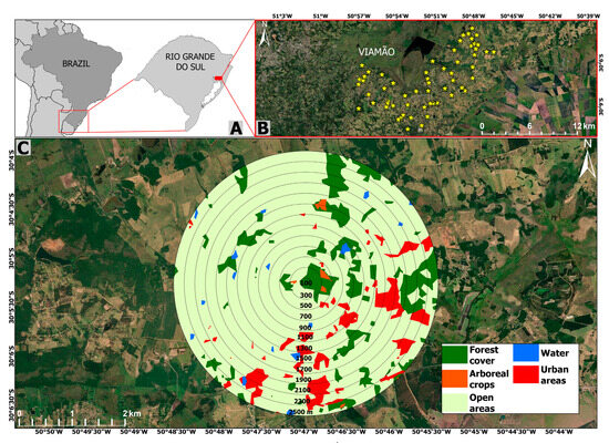
Figure 1.
Location of the study area in Águas Claras district in the state of Rio Grande do Sul, Brazil (A,B). An example of a focal patch and the respective landscape including the 12 buffers around the geographic center of the focal patch is provided in (C).
2.2. Selection of the Study Patches
We defined our study area by creating a 3-km buffer around the RVSBP, covering ca. 15,000 ha (Supplementary Material Figure S1). We mapped all potential brown howler monkey habitat patches using the image bank of the Google Earth Pro© 7.1 software. We considered as potential habitat for the species any patch that presented the minimum requirements for the survival of Alouatta spp. according to other studies, such as a continuous or semi-continuous canopy with an area ≥0.2 ha and an average height ≥10 m [64,65,66]. We manually mapped all patches before the census to specify patch areas and verified heights in situ during fieldwork. We considered patches whose borders were distant at least 50 m from the borders of other patches as independent [67].
We identified 59 potential habitat patches for brown howlers in the study area using the ArcGis 10.6.1 (Environmental System Research Institute, Inc., Redlands, CA, USA) and QGIS 2.14.5 (www.qgis.org) software (Supplementary Material Figure S1). Four of these patches were the aforementioned largest RVSBP forest patches. We used a Garmin® Etrex Legend HCx GPS, Garmin International, Inc., Olathe, KS, USA (geographic coordinates—Datum WGS 94) to confirm in situ the characteristics of the 59 patches.
2.3. Brown Howler Monkey Surveys
We censused brown howlers in the 59 potential habitat patches from March 2014 to March 2016 through active search and direct records (sighting), walking in a way that covered the largest possible area of each patch. We visited each patch in the morning or afternoon at least three times on different dates. Walking speed (ca. 1.0–1.5 km/h) and searching time varied depending on the size of the forest patch and the relief of the terrain. Searching time was never shorter than 3 h on each visit when the monkeys were not sighted. All records of species presence were based on sightings without the need to rely on indirect cues such as calls and fecal remains. However, we heard no calls and found no new or old fecal remains in the forest fragments where howler monkeys were classified as absent, most of which were small. GPH conducted all surveys, often accompanied by PBES.
2.4. Landscape Metrics
We used the open access maps of MapBiomas-Collection 6 (i.e., a 30 m resolution map of Brazil; [68]) to extract landscape variables. We first reclassified these maps to assign five land covers: (1) forest cover, (2) arboreal crops, (3) open areas, (4) urban areas, and (5) water. Forest cover was extracted from the MapBiomas ‘forest formation’ class, which includes dense, open, and mixed ombrophilous forest, semideciduous and deciduous seasonal forests, and secondary forests. Arboreal crops were extracted from the class ‘forest plantation’ and refers to farm-planted forest of commercial tree species. We pooled the classes ‘grassland’, ‘wetland’, ‘agriculture’, and ‘mosaic of agriculture and grassland’ to assign the category open areas. We extracted the urban areas from the classes ‘urban area’, and ‘other non-vegetated areas’. Finally, we extracted water from the class ‘water’, which includes water bodies such as rivers, lakes, oceans, dams, and other reservoirs.
We calculated six landscape predictor variables using ArcGIS 10.5 software: forest cover, patch density, and the amounts of arboreal crops, open areas, urban areas, and water in the matrix. These landscape predictors have been demonstrated to have key relevance for different vertebrates [10,69], including primates [54]. Forest cover refers to the percentage of forest in the landscape. As brown howlers are a forest-dependent species, we used landscape forest cover as a proxy for habitat amount. Including habitat amount (i.e., percentage of forest cover in the landscape) in the models allowed us to statistically assess the independent effects of fragmentation [10]. We used forest-patch density (number of patches in the landscape/total landscape area) because it is one of the most common descriptors of landscape fragmentation per se (i.e., controlling for the effect of forest cover) [10,24], and has been widely used in landscape fragmentation research [6,54,70]. Finally, we used the amount of each of the other four land covers in the matrix to independently evaluate whether and how each affects the occurrence of the study species. We included the effect of matrix composition because of the growing recognition of its role in mediating species responses to landscape changes, including primates [5,71].
We identified the scale of effect for all landscape predictors because we do not know a priori which is the optimal landscape size to assess species–landscape relationships. This assessment is a methodological step needed in studies with a landscape perspective. It is important because species responses to landscape predictors can be overlooked if analyzed at the wrong scale [72,73,74]. Using scales too narrow in range and too few can lead to failing to identify the scale of effect and, thus, losing important species–landscape relationships [74]. Therefore, we created 13 spatial scales (i.e., buffers) ranging from 100 to 2500 m in radii at 200-m intervals from the center of each study site. All of the landscapes with a radius ≥500 m were larger than the maximum reported home range of brown howlers (70 ha; [48]). Although some of our landscapes overlap in the largest buffers, empirical results and simulation studies have demonstrated that overlapping landscapes do not violate the principle of independence and do not induce residual spatial autocorrelation [75,76,77].
2.5. Data Analyses
We used the variance inflation factor (VIF) to assess multicollinearity among landscape predictors using the ‘car’ package [78]. We did not find any strong multicollinearity (maximum VIF = 2.73) [79]. We performed 13 logistic regressions (Generalized Linear Models) for each landscape predictor at each spatial scale. The scale of effect was the landscape scale with the best fit among all models, which we assessed using the lowest Akaike’s information criterion (AIC) [53].
We used Generalized Lineal Models (GLMs) to evaluate the effect of each landscape predictor on the occurrence of brown howlers. We used an information–theoretic approach and multimodel inference to assess the relative effect of each predictor on the response variable [80] using the ‘glmulti’ package [81]. For each model, we computed the Akaike’s information criterion corrected for small samples (AICc), and we ranked the models from best to worst. We employed Akaike weights (wi) to determine the empirical support for each predictor and to generate model-averaged parameter estimates [82]. Therefore, we summed the wi values of ranked models until the total reached 0.95. The set of models for which Pwi was 0.95 represents a group that has a 95% probability of comprising the true optimal model [80]. Finally, we tested for spatial autocorrelation using Moran’s Index. This method measures spatial autocorrelation of model residuals and ranges between −1 (perfectly dispersed) and 1 (perfectly clustered), with 0 being randomly dispersed. We found no significant correlation (Moran I = −0.03, p = 0.63; [83]). We used the software R 3.0.1 for all analyses [84].
3. Results
Considering the respective scale of effect used to assess the effects of each landscape predictor on howler monkey occurrence, the percentage of forest cover in the landscape (scale of effect = 500 m) ranged from <1 to 89%, forest patch density (1900 m) ranged from 0.02 to 0.05 patches/ha, arboreal crops (2500 m) from <1 to 86%, open areas (300 m) from 3 to 99%, urban areas (500 m) from 0 to 48%, and water (1900 m) from <1 to 10%.
Brown howlers inhabited 39 of the 59 study patches (66% occupancy). The model including all landscape predictors explained 39% of the variance (i.e., deviance explained) in the occurrence of howlers (Figure 2). Occurrence was higher in areas with more water in the landscape (Pwi = 0.95; Figure 3a), and lower in areas with more urban (Pwi = 0.91; Figure 3b) and open areas (Pwi = 0.67; Figure 3c). Brown howler occurrence was also positively related to the amount of forest cover in the landscape (Pwi = 0.48; Figure 3d) and negatively related to the area of arboreal crops (Pwi = 0.34; Figure 3e). Finally, we could not assess the direction of the effects of patch density because the unconditional variance was greater than the model-averaged parameter estimate (Table 1; Pwi = 0.22; Figure 3f). This result suggests high variability in the effects of patch density, which can include positive, negative, and null effects. These effects also had the lowest relative importance on the variance of howler monkey occurrence.
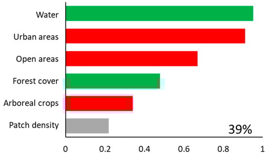
Figure 2.
Predictor variables included in the 95% set of models (bars). The importance of each variable is shown by the sum of Akaike weights (∑wi, panels). The percentage of deviance explained by the complete model (goodness-of-fit) is also indicated. A green bar represents a positive effect of the predictor, a red bar represents a negative effect, and a gray bar indicates that the unconditional variance was higher than the model-averaged estimate, indicating that the parameter may have positive, negative, or no effects, and suggesting caution with interpretations.
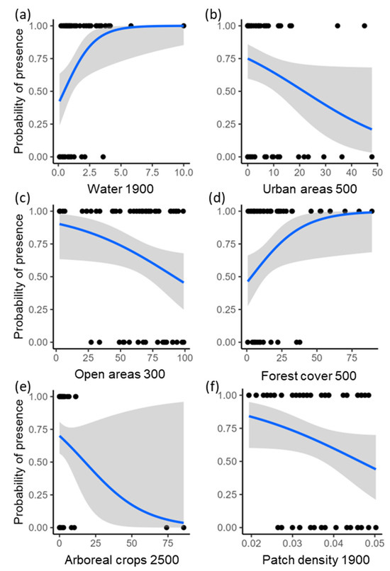
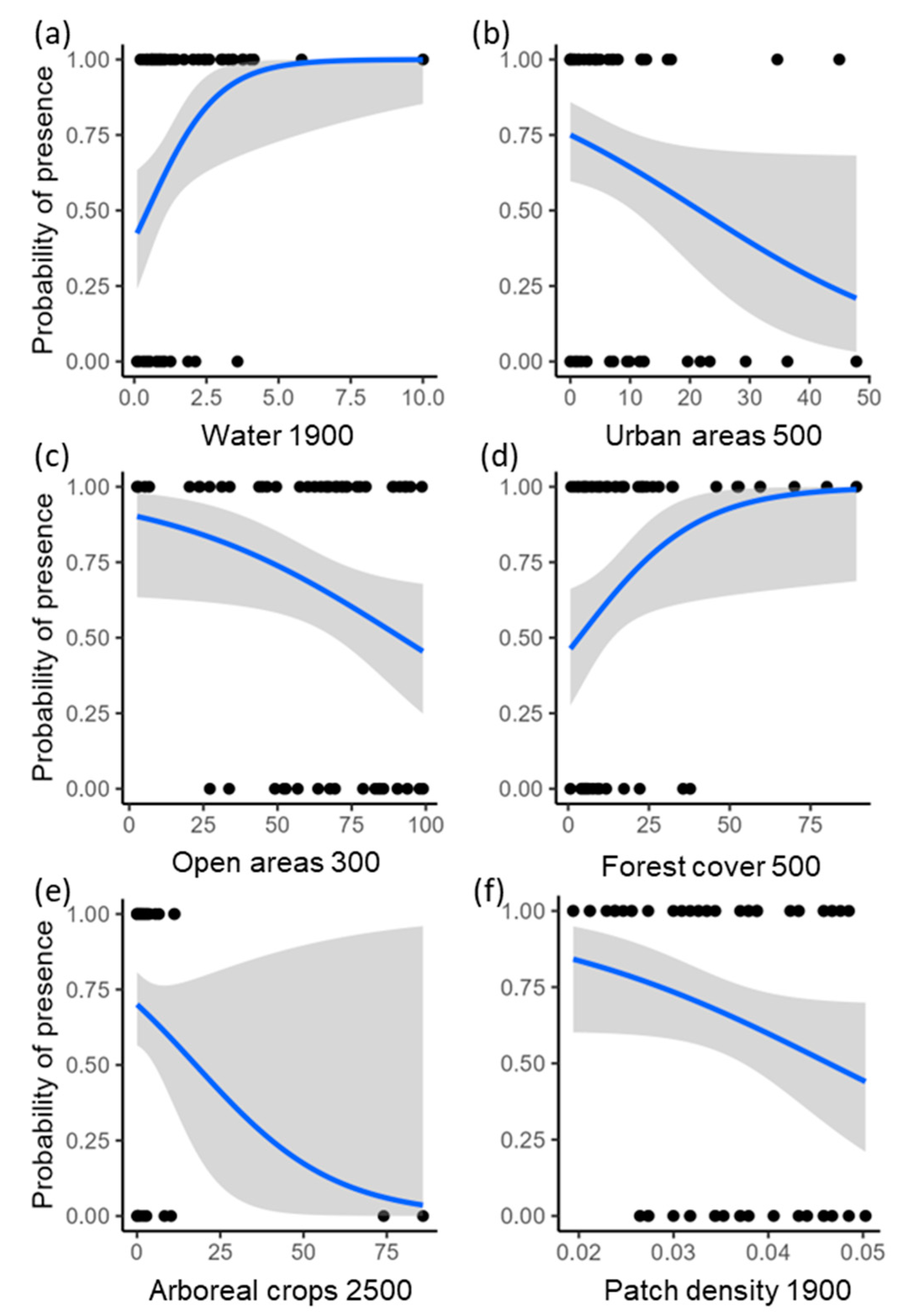
Figure 3.
Relationships between howler monkey occurrence and each landscape predictor at the scale of effect detected for each landscape variable. Points represent the study sites; blue lines indicate the predicted estimates from the logistic regression; and gray areas show the 95% confidence intervals. Numbers on the x-axis represent the scales of effect, i.e., landscape radii from the center of the study patches in meters, identified to assess the effect of each landscape predictor on the occurrence of the brown howler monkey.

Table 1.
Values of model-averaged parameter estimates (β) and unconditional variance (UV) of information–theoretic-based model selection and multimodel inference for each landscape predictor of the occurrence of brown howler monkeys.
4. Discussion
In this study we assessed the effects of landscape structure on the occurrence of brown howler monkeys near the southern limit of the species’ distribution [59]. Contrary to our predictions, the occurrence of brown howlers was higher in landscapes with more water and lower in landscapes with more arboreal crops. As expected, howler occurrence was positively related to forest cover and inversely related to urban and open areas in the landscape. Finally, we could not determine the specific effect of fragmentation per se on the occurrence of brown howlers because its effects were highly variable.
The unexpected positive relationship between the occurrence of howler monkeys and its most important landscape predictor, the amount of water, which accounted for quite a small cover of each landscape, may have been influenced by a combination of factors. On one hand, landscapes with higher amounts of water are characterized by more rural areas with lower urbanization and less farming, which tend to have a lower frequency of electrocution, roadkill, and dog attacks [31,32,33,37,85]. Such reduced risk of monkey mortality leads to higher patch occupancy. This explanation is supported by the lower occurrence of brown howlers in habitat patches immersed in landscapes with more urban areas and more open areas (the second- and third-best predictors of the species’ presence), which normally lack their food resources or arboreal refuges (but see [86,87]). On the other hand, our result may be influenced by the species’ presence in the four medium-to-large forest patches of the RVSBP wildlife refuge, which consists partially of wetlands that may be misclassified as water by MapBiomas. Therefore, relatively high forest cover in these landscapes may also be positively related to patch occupancy.
The empirical demonstration of forest cover as an important predictor of patch occupancy by brown howlers in the study area is explained by its direct relationship with resource availability, as reported elsewhere [10]. Larger areas of habitat also increase connectivity, reducing the use of ground to move between isolated patches or to visit supplementary food sources in the matrix, thereby avoiding the aforementioned risks and increasing the likelihood of long-term population survival. In fact, habitat loss (or forest loss for forest specialists) is considered the most significant threat to species persistence worldwide [10,12,88,89]. This is also applicable to howler monkeys. Despite being a disturbance-tolerant arboreal species capable of coping with some degree of habitat loss, they may face compromised long-term persistence in deforested landscapes [90].
The also unexpected finding that a greater cover of arboreal crops in the landscape correlates with a lower presence of howler monkeys might be attributed to the fact that this land cover in the study area consists predominantly of Pinus spp. and Eucalyptus spp. [68]. Trees belonging to these genera are uncommon food sources for brown howlers [46]. Plant diversity in these plantations tends to be quite low and, therefore, it is expected that brown howlers are not attracted to them. Plantations that are connected to patches of remnant native forest or that contain native trees regenerating under the cultivated trees or vines growing on them, however, may attract howler monkeys as reported for Alouatta pigra in Mexico [91]. It is important to note that MapBiomas may not classify small isolated orchards near rural properties that are known to play a positive role as sources of supplementary food for howler monkeys [92] as arboreal crops. This methodological limitation may have influenced both the direction of the relationship between this matrix land cover and the occurrence of brown howlers in the forest patches. It is also possible that there is greater human presence near arboreal crops, a condition that is expected to increase the level of stress and the frequency of the direct causes of howler monkey death mentioned above, both with negative consequences for the persistence of the species in the landscape.
The direction of the effects of fragmentation per se (i.e., independent of the effect of habitat amount) on the occurrence of the brown howler monkey were not clear. This is because the unconditional variance of patch density was greater than the model-averaged parameter estimate, which indicates a high degree of variability in the effect of patch density across the models and suggests that the effects of patch density are highly variable, encompassing positive, null, and negative effects. Our result points to a complex relationship between patch density and howlers’ occupancy, indicating that the effect of patch density is not consistent. Similar to studies of Brazilian primate richness [54], sapling assemblages [93], and tree seed dispersal [94], these results align with substantial empirical evidence that fragmentation per se generally has weak effects on most species [24,95,96,97]. These weak effects imply that habitat configuration is less critical for species survival in anthropogenic landscapes than landscape composition, such as the amount of habitat. In our study, these weak effects mean that the number of forest patches does not affect the persistence of brown howlers in landscapes with the same total amount of forest.
We assessed the effects of landscape matrix covers separately. A common approach to assess the effects of the matrix on species is to use an index of matrix quality or functionality based on a subjective, researcher-focused perception of the ability of target species to use land covers for feeding or travelling [54,98,99]. This is particularly critical when our understanding of how the species use or interact with land covers in the matrix is scarce [100], and that is precisely when we call on these indices. Therefore, it is urgent to increase our understanding of how landscape attributes affect species persistence in anthropogenic landscapes especially for highly threatened species, such as primates [90,101].
Finally, the shorter scales of effect for forest cover, open areas, and urban areas are consistent with the 200 m threshold for efficient dispersal through a non-forest matrix by mantled howler monkeys (Alouatta palliata [102]). This is also consistent with the distance often traveled by brown howlers in a single day (mean day range = 620 m, SD = 142, N = 21 studies; [48]), and the restriction of gene flow caused by open areas between isolated populations of black-and-gold howler monkeys (Alouatta caraya) [103]. On the contrary, the much larger scales of effect for water, arboreal crops, and patch density exceeded the longest day range recorded to date (1677 m) and covered areas >16 times larger than the maximum reported home range of brown howlers (70 ha) and >87 times larger than their mean home range (13 ha; [48]). This indicates that these predictors influence the occurrence of brown howlers through processes other than species dispersal, such as regional processes. Yet, further studies are needed to understand what determines the scale of effect [104].
5. Conclusions
Our study highlights the critical impact of landscape composition on brown howler monkey occurrence in the studied anthropogenic landscapes, with the particular importance of both protecting the remaining forest patches and promoting forest restoration to save the species and the coexisting native wildlife as recently proposed for primates in general [105]. We suggest that the future of brown howler monkeys and other species with similar ecological requirements in anthropogenic landscapes with comparable human demographic and environmental characteristics will require the implementation of measures to reduce the impact of conflicts on populations. These measures include lowering the speed of vehicles, installing wildlife-friendly power lines, managing the number of stray dogs in the landscape, and enforcing antipoaching laws. This recommendation is particularly urgent considering the increasing urban encroachment on natural ecosystems resulting from the growing human population [34]. Forest protection and restoration are crucial strategies for mitigating the effects of habitat destruction for forest-specialist species.
Supplementary Materials
The following supporting information can be downloaded at: https://www.mdpi.com/article/10.3390/land13040514/s1, Figure S1: Location of the study area in the Águas Claras district in the state of Rio Grande do Sul, Brazil. Forest patches inhabited by howler monkeys are marked in yellow, whereas non-inhabited patches are marked in red; Figure S2: Locations of the study patches in the Águas Claras district in the state of Rio Grande do Sul, Brazil. The smallest buffers per patch used after identifying the scale of effect (with a 300-m radius) are shown in yellow, and the largest buffer (with a 2500-m radius) are shown in white.
Author Contributions
J.C.B.-M. conceived and designed the study; G.P.H. and P.B. conducted the censuses; V.K. extracted the landscape metrics; and C.G.-A. conceived and performed the data analysis, and wrote the first draft of the manuscript. All authors contributed to and edited the other versions of the manuscript. All authors have read and agreed to the published version of the manuscript.
Funding
VK was supported by a PhD fellowship from National Council for Scientific and Technological Development/CNPq (nr 140674/2020-9) and J.C.B.-M. was supported with a Research Productivity Scholarship (PQ 1C, n° 303306/2013-0). The data collection was partially supported by the Pró-Reitoria de Pesquisa e Pós-Graduação from the Pontifical Catholic University of Rio Grande do Sul, PUCRS.
Institutional Review Board Statement
This research was purely observational and all observations were made in accordance with Brazilian laws. The research met all ethical recommendations of the International Primatological Society’s and American Society of Primatologists’ Code of Good Practices for Field Primatology. Our research protocol was approved by the Office of the Dean of Research and Graduate Studies of the Pontifical Catholic University of Rio Grande do Sul.
Data Availability Statement
The original data presented in the study are openly available in FigShare at https://figshare.com/articles/dataset/Dataset_for_Galán-Acedo_et_al_2024_Urban_matrices_threaten_patch_occurrence_of_howler_monkeys_in_anthropogenic_landscapes_Land_/25590495 accessed on February 2024.
Acknowledgments
We thank Regis Alexandre Lahm and Everton Luis Luz de Quadros for running a previous analysis of the spatial data.
Conflicts of Interest
The authors have no relevant financial or non-financial interests to disclose.
References
- Van Vliet, J. Direct and indirect loss of natural area from urban expansion. Nat. Sustain. 2019, 2, 755–763. [Google Scholar] [CrossRef]
- Newbold, T.; Hudson, L.N.; Arnell, A.P.; Contu, S.; De Palma, A.; Ferrier, S.; Hill, S.L.L.; Hoskins, A.J.; Lysenko, I.; Phillips, H.R.P.; et al. Has land use pushed terrestrial biodiversity beyond the planetary boundary? A global assessment. Science (80-). 2016, 353, 288–291. [Google Scholar] [CrossRef]
- Pinzón, X.C. Uso de cercas vivas como corredores biológicos por primates en los llanos orientales. In Primatología en Colombia: Avances al Principo del Milenio; Pereira-Bengoa, V., Stevenson, P.R., Bueno, M.L., Nassar-Montoya, F., Eds.; Fundación Universitaria San Martín: Bogota, Colombia, 2010; pp. 91–97. [Google Scholar]
- Threlfall, C.G.; Law, B.; Banks, P.B. Influence of landscape structure and human modifications on insect biomass and bat foraging activity in an urban landscape. PLoS ONE 2012, 7, e38800. [Google Scholar] [CrossRef]
- Galán-Acedo, C.; Arroyo-Rodríguez, V.; Estrada, A.; Ramos-Fernández, G. Forest cover and matrix functionality drive the abundance and reproductive success of an Endangered primate in two fragmented rainforests. Landsc. Ecol. 2019, 34, 147–158. [Google Scholar] [CrossRef]
- Gestich, C.C.; Arroyo-Rodríguez, V.; Saranholi, B.H.; da Cunha, R.G.T.; Setz, E.Z.F.; Ribeiro, M.C. Forest loss and fragmentation can promote the crowding effect in a forest-specialist primate. Landsc. Ecol. 2021, 37, 147–157. [Google Scholar] [CrossRef]
- Pellissier, V.; Cohen, M.; Boulay, A.; Clergeau, P. Birds are also sensitive to landscape composition and configuration within the city centre. Landsc. Urban Plan. 2012, 104, 181–188. [Google Scholar] [CrossRef]
- Martin, L.J.; Blossey, B.; Ellis, E. Mapping where ecologists work: Biases in the global distribution of terrestrial ecological observations. Front. Ecol. Environ. 2012, 10, 195–201. [Google Scholar] [CrossRef]
- Di Marco, M.; Ferrier, S.; Harwood, T.D.; Hoskins, A.J.; Watson, J.E.M. Wilderness areas halve the extinction risk of terrestrial biodiversity. Nature 2019, 573, 582–585. [Google Scholar] [CrossRef]
- Fahrig, L. Effects of habitat fragmentation on biodiversity. Annu. Rev. Ecol. Evol. Syst. 2003, 34, 487–515. [Google Scholar] [CrossRef]
- Arroyo-Rodríguez, V.; Fahrig, L.; Tabarelli, M.; Watling, J.I.; Tischendorf, L.; Benchimol, M.; Cazetta, E.; Faria, D.; Leal, I.-R.; Melo, F.P.L.; et al. Designing optimal human-modified landscapes for forest biodiversity conservation. Ecol. Lett. 2020, 23, 1404–1420. [Google Scholar] [CrossRef]
- Watling, J.I.; Arroyo-Rodríguez, V.; Pfeifer, M.; Baeten, L.; Banks-Leite, C.; Cisneros, L.M.; Fang, R.; HamelLeigue, A.C.; Lachat, T.; Leal, I.R.; et al. Support for the habitat amount hypothesis from a global synthesis of species density studies. Ecol. Lett. 2020, 23, 674–681. [Google Scholar] [CrossRef]
- Haddad, N.M.; Brudvig, L.A.; Clobert, J.; Davies, K.F.; Gonzalez, A.; Holt, R.D.; Lovejoy, T.E.; Sexton, J.O.; Austin, M.P.; Collins, C.D.; et al. Habitat fragmentation and its lasting impact on Earth’s ecosystems. Sci. Adv. 2015, 1, e1500052. [Google Scholar] [CrossRef]
- Keesing, F.; Ostfeld, R.S. Impacts of biodiversity and biodiversity loss on zoonotic diseases. Proc. Natl. Acad. Sci. USA 2021, 118, e2023540118. [Google Scholar] [CrossRef]
- Li, Y.; Bearup, D.; Liao, J. Habitat loss alters effects of intransitive higher-order competition on biodiversity: A new metapopulation framework. Proc. R. Soc. B 2020, 287, 20201571. [Google Scholar] [CrossRef]
- Naug, D. Nutritional stress due to habitat loss may explain recent honeybee colony collapses. Biol. Conserv. 2009, 142, 2369–2372. [Google Scholar] [CrossRef]
- Fahrig, L.; Arroyo-Rodríguez, V.; Bennett, J.R.; Boucher-Lalonde, V.; Cazetta, E.; Currie, D.J.; Eigenbrod, F.; Ford, A.T.; Harrison, S.P.; Jaeger, J.A.G.; et al. Is habitat fragmentation bad for biodiversity? Biol. Conserv. 2019, 230, 179–186. [Google Scholar] [CrossRef]
- Fletcher, R.J., Jr.; Didham, R.K.; Banks-Leite, C.; Barlow, J.; Ewers, R.M.; Rosindell, J.; Al, E. Is habitat fragmentation good for biodiversity? Biol. Conserv. 2018, 226, 9–15. [Google Scholar] [CrossRef]
- Bascompte, J.; Solé, R.V. Habitat fragmentation and extinction thresholds in spatially explicit models. J. Anim. Ecol. 1996, 65, 465–473. [Google Scholar] [CrossRef]
- Hanski, I. Metapopulation dynamics. Nature 1998, 396, 41–49. [Google Scholar] [CrossRef]
- Martin, C.A. An early synthesis of the habitat amount hypothesis. Landsc. Ecol. 2018, 33, 1831–1835. [Google Scholar] [CrossRef]
- De Camargo, R.X.; Boucher-Lalonde, V.; Currie, D.J. At the landscape level, birds respond strongly to habitat amount but weakly to fragmentation. Divers. Distrib. 2018, 24, 629–639. [Google Scholar] [CrossRef]
- Arroyo-Rodríguez, V.; Fahrig, L. Why is a landscape perspective important in studies of primates? Am. J. Primatol. 2014, 76, 901–909. [Google Scholar] [CrossRef]
- Fahrig, L. Ecological responses to habitat fragmentation per se. Annu. Rev. Ecol. Evol. Syst. 2017, 48, 1–23. [Google Scholar] [CrossRef]
- Galán-Acedo, C.; Arroyo-Rodríguez, V.; Cudney-Valenzuela, S.J.; Fahrig, L. A global assessment of primate responses to landscape structure. Biol. Rev. 2019, 94, 1605–1618. [Google Scholar] [CrossRef]
- Galán-Acedo, C.; Arroyo-Rodríguez, V.; Andresen, E.; Arregoitia, L.V.; Vega, E.; Peres, C.A.; Ewers, R.M. The conservation value of human-modified landscapes for the world’s primates. Nat. Commun. 2019, 10, 152. [Google Scholar] [CrossRef]
- Ramírez-Delgado, J.P.; Di Marco, M.; Watson, J.E.; Johnson, C.J.; Rondinini, C.; Corredor-Llano, X.; Arias, M.; Venter, O. Matrix Condition Mediates the Effects of Habitat Fragmentation on Species Extinction Risk. Nat. Commun. 2022, 13, 1–10. [Google Scholar] [CrossRef]
- Forman, R. Land Mosaics: The Ecology of Landscapes and Regions; Cambridge Univ Press: New York, NY, USA, 1995. [Google Scholar]
- Ferreira, A.S.; Peres, C.A.; Bogoni, J.A.; Cassano, C.R. Use of agroecosystem matrix habitats by mammalian carnivores (Carnivora): A global-scale analysis. Mamm. Rev. 2018, 48, 312–327. [Google Scholar] [CrossRef]
- Prevedello, J.A.; Vieira, M.V. Does the type of matrix matter? A quantitative review of the evidence. Biodivers. Conserv. 2010, 19, 1205–1223. [Google Scholar] [CrossRef]
- Fahrig, L.; Baudry, J.; Brotons, L.; Burel, F.G.; Crist, T.O.; Fuller, R.J.; Sirami, C.; Siriwardena, G.M.; Martin, J.L. Functional landscape heterogeneity and animal biodiversity in agricultural landscapes. Ecol. Lett. 2011, 14, 101–112. [Google Scholar] [CrossRef]
- Devictor, V.; Julliard, R.; Jiguet, F. Distribution of specialist and generalist species along spatial gradients of habitat disturbance and fragmentation. Oikos 2008, 117, 507–514. [Google Scholar] [CrossRef]
- Perfecto, I.; Vandermeer, J. Biodiversity conservation in tropical agroecosystems: A new conservation paradigm. Ann. N. Y. Acad. Sci. 2008, 1134, 173–200. [Google Scholar] [CrossRef]
- Corrêa, F.M.; Chaves, Ó.M.; Printes, R.C.; Romanowski, H.P. Surviving in the urban–rural interface: Feeding and ranging behavior of brown howlers (Alouatta guariba clamitans) in an urban fragment in southern Brazil. Am. J. Primatol. 2018, 80, 1–12. [Google Scholar] [CrossRef]
- Petrucci, M.P.; Pontes, L.A.; Queiroz, F.F.; Cruz, M.C.; Souza, D.B.; Silveira, L.S.; Rodrigues, A.B. Electrocution accident in free-ranging bugio (Alouatta fusca) with subsequent amputation of the forelimb: Case report. Rev. Port. Ciências Veterinárias 2009, 104, 104–113. [Google Scholar]
- Rytwinski, T.; Fahrig, L. The impacts of roads and traffic on terrestrial animal populations. In Handbook of Road Ecology; Wiley: Hoboken, NJ, USA, 2015; pp. 237–246. [Google Scholar]
- Chaves, O.; Souza, J.; Buss, G.; Hirano, Z.; Jardim, M.; Amaral, E.; Godoy, J.; Peruchi, A.; Michel, T.; Bicca-Marques, J.C. Wildlife is imperiled in peri-urban landscapes: Threats to arboreal mammals. Sci. Total Environ. 2022, 821, 152883. [Google Scholar] [CrossRef]
- Mittermeier, R.A.; Rylands, A.B.; Hoyo, J.D.; Anandam, M. Handbook of the Mammals of the World; Mittermeier, R.A., Rylands, A.B., Wilson, D.E., Eds.; Lynx Edicions: Barcelona, Spain, 2013; Volume 3. [Google Scholar]
- IUCN International Union for Conservation of Nature. IUCN Red List of Threatened Species; Version 2024; IUCN: Geneva, Switzerland, 2024. [Google Scholar]
- Estrada, A.; Garber, P.A.; Rylands, A.B.; Roos, C.; Fernandez-Duque, E.; Di Fiore, A.; Nekaris, K.A.-I.; Nijman, V.; Heymann, E.W.; Lambert, J.E.; et al. Impending extinction crisis of the world’s primates: Why primates matter. Sci. Adv. 2017, 3, e1600946. [Google Scholar] [CrossRef]
- Galea, B.; Humle, T. Identifying and mitigating the impacts on primates of transportation and service corridors. Conserv. Biol. 2022, 36, e13836. [Google Scholar] [CrossRef]
- Marsh, L.K.; Chapman, C.A.; Arroyo-Rodríguez, V.; Cobden, A.K.; Dunn, J.C.; Gabriel, D.; Ghai, R.; Nijman, V.; Reyna-Hurtado, R.; Serio-silva, J.C.; et al. Primates in fragments 10 years later: Once and future goals. In Primates in Fragments; Marsh, L.K., Chapman, C.A., Eds.; Springer: New York, NY, USA, 2013; pp. 505–525. ISBN 978-1-4757-3772-1. [Google Scholar]
- Andresen, E.; Arroyo-Rodríguez, V.; Ramos-Robles, M. Primate seed dispersal: Old and new challenges. Int. J. Primatol. 2018, 39, 443–465. [Google Scholar] [CrossRef]
- Chapman, C.A.; Bonnell, T.R.; Gogarten, J.F.; Lambert, J.E.; Omeja, P.A.; Twinomugisha, D.; Wasserman, M.D.; Rothman, J.M. Are primates ecosystem engineers? Int. J. Primatol. 2013, 34, 1–14. [Google Scholar] [CrossRef]
- Buss, G.; Bicca-Marques, J.C.; Alves, S.L.; Ingberman, B.; Fries, B.G.; Alonso, A.C.; da Cunha, R.; Miranda, J.; de Melo, F.; Jerusalinsky, L.; et al. Alouatta guariba ssp. clamitans (amended version of 2020 assessment). In The IUCN Red List of Threatened Species, 2021; IUCN: Geneva, Switzerland, 2021. [Google Scholar]
- Chaves, Ó.M.; Bicca-Marques, J.C. Dietary flexibility of the brown howler monkey throughout its geographic distribution. Am. J. Primatol. 2013, 75, 16–29. [Google Scholar] [CrossRef]
- Chaves, Ó.M.; Bicca-Marques, J.C. Feeding strategies of brown howler monkeys in response to variations in food availability. PLoS ONE 2016, 11, e0145819. [Google Scholar] [CrossRef]
- Fortes, V.B.; Bicca-Marques, J.C.; Urbani, B.; Fernández, V.A.; da Silva Pereira, T. Ranging behavior and spatial cognition of howler monkeys. In Howler Monkeys; Kowalewski, M.M., Garber, P.A., Cortés-Ortiz, L., Urbani, B., Youlatos, D., Eds.; Springer: New York, NY, USA, 2015; pp. 219–255. [Google Scholar]
- Chaves, Ó.M.; Bicca-Marques, J.C. Crop-feeding by brown howler monkeys (Alouatta guariba clamitans) in forest fragments: The conservation value of cultivated species. Int. J. Primatol. 2017, 38, 263–281. [Google Scholar] [CrossRef]
- Lopes, S.; Calegaro-Marques, C.; Klain, V.; Chaves, Ó.M.; Bicca-Marques, J.C. Necropsies disclose a low helminth parasite diversity in periurban howler monkeys. Am. J. Primatol. 2022, 84, e23346. [Google Scholar] [CrossRef]
- Rêgo, P.R.; Schipper, J.; dos Reis, S.F.; Ferrari, S.F.; Siqueira, M.F. How much of the Atlantic Forest is needed to conserve the southern brown howler monkey, Alouatta guariba clamitans? Biol. Conserv. 2015, 191, 11–18. [Google Scholar]
- Possamai, C.B.; Melo, F.R.; Mendes, S.L.; Strier, K.B. Demographic changes in an Atlantic Forest primate community following a yellow fever outbreak. Am. J. Primatol. 2022, 84, e23425. [Google Scholar] [CrossRef]
- Jackson, H.B.; Fahrig, L. What size is a biologically relevant landscape? Landsc. Ecol. 2012, 27, 929–941. [Google Scholar] [CrossRef]
- Galán-Acedo, C.; Spaan, D.; Bicca-Marques, J.C.; de Azevedo, R.B.; Villalobos, F.; Rosete-Vergés, F. Regional deforestation drives the impact of forest cover and matrix quality on primate species richness. Biol. Conserv. 2021, 263, 109338. [Google Scholar] [CrossRef]
- Bicca-Marques, J.C. Primates in Fragments; Springer: Berlin/Heidelberg, Germany, 2003. [Google Scholar]
- Prates, H.M.; Bicca-Marques, J.C. Age-sex analysis of activity budget, diet, and positional behavior in Alouatta caraya in an orchard forest. Int. J. Primatol. 2008, 29, 703–715. [Google Scholar] [CrossRef]
- Azevedo, R.B.; Bicca-Marques, J.C. Posturas de alimentação e tipos de locomoção em bugios-ruivos (Alouatta guariba clamitans) em ambiente natural. In A Primatologia no Brasil; Bicca-Marques, J.C., Ed.; Sociedade Brasileira de Primatologia: Porto Alegre, Brazil, 2007; pp. 375–385. [Google Scholar]
- Seto, K.C.; Güneralp, B.; Hutyra, L.R. Global forecasts of urban expansion to 2030 and direct impacts on biodiversity and carbon pools. Proc. Natl. Acad. Sci. USA 2012, 109, 16083–16088. [Google Scholar] [CrossRef]
- Culot, L.; Pereira, L.A.; Agostini, I.; De Almeida, M.A.B.; Alves, R.S.C.; Aximoff, I.; Braga, C. Atlantic-Primates: A dataset of communities and occurrences of primates in the Atlantic Forests of South America. Ecology 2019, 100, e02525. [Google Scholar] [CrossRef]
- Instituto Nacional de Meteorologia. Históricos de Dados Meteorológicos; Instituto Nacional de Meteorologia: Porto Alegre, Brazil, 2002. [Google Scholar]
- Hasenack, H.; Weber, E.; Boldrini, I.I.; Trevisan, R. Mapa de Sistemas Ecológicos da Ecorregião das Savanas Uruguaias em Escala 1: 500.000 ou Superior e Relatório Técnico Descrevendo Insumos Utilizados e Metodologia de Elaboração do Mapa de Sistemas Ecológicos; UFGRS: Porto Alegre, Brazil, 2010. [Google Scholar]
- Bauermann, S.G. Análises palinologicas e evolucao paleovegetacional e paleoambiental das turfeiras de Barrocadas e Aguas Claras. In Planície Costeira do Rio Grande do Sul, Brasil; Universidade Federal do Rio Grande do Sul: Rio Grande, Brazil, 2003. [Google Scholar]
- Rosa, A.O. Refúgio de Vida Silvestre Banhado dos Pachecos: Plano de Manejo; Secretaria do Meio Ambiente e Infraestrutura: Porto Alegre, Brazil, 2022. [Google Scholar]
- Anzures-Dadda, A.; Manson, R.H. Patch- and landscape-scale effects on howler monkey distribution and abundance in rainforest fragments. Anim. Conserv. 2007, 10, 69–76. [Google Scholar] [CrossRef]
- Pozo-Montuy, G.; Serio-Silva, J.C.; Bonilla-Sánchez, Y.M. Influence of the landscape matrix on the abundance of arboreal primates in fragmented landscapes. Primates 2011, 52, 139–147. [Google Scholar] [CrossRef]
- Mandujano, S.; Escobedo-Morales, L.A.; Palacios-Silva, R.; Arroyo-Rodríguez, V.; Rodríguez-Toledo, E.M. A metapopulation approach to conserving the howler monkey in a highly fragmented landscape in Los Tuxtlas, Mexico. In New Perspectives in the Study of Mesoamerican Primates: Distribution, Ecology, Behavior, and Conservation; Estrada, A., Garber, P.A., Pavelka, M.S.M., Luecke, L., Eds.; Kluwer Academic/Plenum Publishers: New York, NY, USA, 2006; pp. 513–538. [Google Scholar]
- Onderdonk, D.A.; Chapman, C.A. Coping with forest fragmentation: The primates of Kibale National Park, Uganda. Int. J. Primatol. 2000, 21, 587–611. [Google Scholar] [CrossRef]
- Souza, C.; Azevedo, T. MapBiomas General Handbook; MapBiomas: São Paulo, Brazil, 2017. [Google Scholar]
- Fahrig, L. Rethinking patch size and isolation effects: The habitat amount hypothesis. J. Biogeogr. 2013, 40, 1649–1663. [Google Scholar] [CrossRef]
- Ordóñez-Gómez, J.D.; Arroyo-Rodríguez, V.; Nicasio-Arzeta, S.; Cristóbal-Azkarate, J. Which is the appropriate scale to assess the impact of landscape spatial configuration on the diet and behavior of spider monkeys? Am. J. Primatol. 2015, 77, 56–65. [Google Scholar] [CrossRef]
- Blanco, V.; Waltert, M. Does the tropical agricultural matrix bear potential for primate conservation? A baseline study from Western Uganda. J. Nat. Conserv. 2013, 21, 383–393. [Google Scholar] [CrossRef]
- Wiens, J.A. Spatial scaling in ecology. Funct. Ecol. 1989, 3, 385–397. [Google Scholar] [CrossRef]
- Holland, J.D.; Bert, D.G.; Fahrig, L. Determining the spatial scale of species’ response to habitat. Bioscience 2004, 54, 227–233. [Google Scholar] [CrossRef]
- Jackson, H.B.; Fahrig, L. Are ecologists conducting research at the optimal scale? Glob. Ecol. Biogeogr. 2015, 24, 52–63. [Google Scholar] [CrossRef]
- Zuckerberg, B.; Desrochers, A.; Hochachka, W.M.; Fink, D.; Koenig, W.D.; Dickinson, J.L. Overlapping landscapes: A persistent, but misdirected concern when collecting and analyzing ecological data. J. Wildl. Manag. 2012, 76, 1072–1080. [Google Scholar] [CrossRef]
- Zuckerberg, B.; Cohen, J.M.; Nunes, L.A.; Bernath-Plaisted, J.; Clare, J.D.; Gilbert, N.A.; Kozidis, S.S.; Nelson, S.B.M.; Shipley, A.A.; Thompson, K.L.; et al. A review of overlapping landscapes: Pseudoreplication or a red herring in landscape ecology? Curr. Landsc. Ecol. Reports 2020, 5, 140–148. [Google Scholar] [CrossRef]
- Arnqvist, G. Mixed models offer no freedom from degrees of freedom. Trends Ecol. Evol. 2020, 35, 329–335. [Google Scholar] [CrossRef]
- Fox, K.; Weisberg, S.; Price, B.; Adler, D.; Bates, D.; Baud-Bovy, G.; Bolker, B.; Ellison, S.; Firth, D.; Friendly, M.; et al. Package ‘car’ 2012; R Foundation for Statistical Computing: Vienna, Austria, 2012. [Google Scholar]
- Neter, J.; Kutner, M.; Nachtsheim, C.; Wassermen, W. Applied Linear Statistical Models, 4th ed.; Irwin: Chicago, IL, USA, 1996. [Google Scholar]
- Burnham, K.; Anderson, D. Model Selection and Multimodel Inference: A Practical Information—Theoretic Approach, 2nd ed.; Springer: New York, NY, USA, 2002. [Google Scholar]
- Calcagno, V.; de Mazancourt, C. Glmulti: An R package for easy automated model selection with (generalized) linear models. J. Stat. Softw. 2010, 34, 1–29. [Google Scholar] [CrossRef]
- Anderson, D.R. Model Based Inference in the Life Sciences: A Primer on Evidence; Anderson, D.R., Ed.; Springer-Verlag: New York, NY, USA, 2007. [Google Scholar]
- Dormann, F.; McPherson, C.M.; Araújo, M.; Bivand, R.; Bolliger, J.; Carl, G.; Davies, R.G.; Hirzel, A.; Jetz, W.; Daniel Kissling, W.; et al. Methods to account for spatial autocorrelation in the analysis of species distributional data: A review. Ecography 2007, 30, 609–628. [Google Scholar] [CrossRef]
- R Core Team. R Version 3.0.1.; R Foundation for Statistical Computing: Vienna, Austria, 2013. [Google Scholar]
- Franklin, J.F. Preserving biodiversity: Species, ecosystems, or landscapes? Ecol. Appl. 1993, 3, 202–205. [Google Scholar] [CrossRef]
- Back, J.P.; Bicca-Marques, J.C. Supplemented howler monkeys eat less wild fruits, but do not change their activity budgets. Am. J. Primatol. 2019, 81, e23051. [Google Scholar] [CrossRef]
- Lima, I.A.; Bicca-Marques, J.C. Opportunistic meat-eating by urban folivorous-frugivorous monkeys. Primates 2024, 65, 25–32. [Google Scholar] [CrossRef]
- Fardila, D.; Kelly, L.T.; Moore, J.L.; McCarthy, M.A. A systematic review reveals changes in where and how we have studied habitat loss and fragmentation over 20 years. Biol. Conserv. 2017, 212, 130–138. [Google Scholar] [CrossRef]
- Pimm, S.L.; Jenkins, C.N.; Abell, R.; Brooks, T.M.; Gittleman, J.L.; Joppa, L.N.; Raven, P.H.; Roberts, C.M.; Sexton, J.O. The biodiversity of species and their rates of extinction, distribution, and protection. Science 2014, 344, 1246752. [Google Scholar] [CrossRef]
- Bicca-Marques, J.C.; Chaves, Ó.M.; Hass, G.P. Howler monkey tolerance to habitat shrinking: Lifetime warranty or death sentence? Am. J. Primatol. 2020, 82, e23089. [Google Scholar] [CrossRef]
- Bonilla-Sánchez, Y.M.; Serio-Silva, J.C.; Pozo-Montuy, G.; Chapman, C.A. Howlers are able to survive in eucalyptus plantations where remnant and regenerating vegetation is available. Int. J. Primatol. 2012, 33, 233–245. [Google Scholar] [CrossRef]
- Pozo-Montuy, G.; Serio-Silva, J.C.; Chapman, C.A.; Bonilla-Sánchez, Y.M. Resource use in a landscape matrix by an arboreal primate: Evidence of supplementation in black howlers (Alouatta pigra). Int. J. Primatol. 2013, 34, 714–731. [Google Scholar] [CrossRef]
- Arasa-Gisbert, R.; Arroyo-Rodríguez, V.; Galán-Acedo, C.; Meave, J.A.; Martínez-Ramos, M. Tree recruitment failure in old-growth forest patches across human-modified rainforests. J. Ecol. 2021, 109, 2354–2366. [Google Scholar] [CrossRef]
- San-José, M.; Arroyo-Rodríguez, V.; Meave, J.A. Regional context and dispersal mode drive the impact of landscape structure on seed dispersal. Ecol. Appl. 2020, 30, e02033. [Google Scholar] [CrossRef]
- Johnson, M.W.; Heck Jr, K.L. Effects of habitat fragmentation per se on decapods and fishes inhabiting seagrass meadows in the northern Gulf of Mexico. Mar. Ecol. Prog. Ser. 2006, 306, 233–246. [Google Scholar] [CrossRef]
- Watz, J.; Eckstein, R.L.; Nyqvist, D. Effects of fragmentation per se on slug movement. Acta Oecologica 2021, 112, 103771. [Google Scholar] [CrossRef]
- Snyder, R. Species Responses to Habitat Edges and Fragmentation per se: A Cross Taxa Meta-Analysis; John Carroll University: Heights, OH, USA, 2023. [Google Scholar]
- Garmendia, A.; Arroyo-Rodríguez, V.; Estrada, A.; Naranjo, E.J.; Stoner, K.E. Landscape and patch attributes impacting medium- and large-sized terrestrial mammals in a fragmented rain forest. J. Trop. Ecol. 2013, 29, 331–344. [Google Scholar] [CrossRef]
- Silva, L.G.; Ribeiro, M.C.; Hasui, E.; Costa, C.A.; Cunha, R.G.T. Patch size, functional isolation, visibility and matrix permeability influences Neotropical primate occurrence within highly fragmented landscapes. PLoS ONE 2015, 10, e0114025. [Google Scholar] [CrossRef] [PubMed]
- McBride, M.F.; Burgman, M.A. What is expert knowledge, how is such knowledge gathered, and how do we use it to address questions in landscape ecology? In Expert Knowledge and Its Application in Landscape Ecology; Springer: New York, NY, USA, 2012; pp. 11–38. [Google Scholar]
- Strier, K.B. The limits of resilience. Primates 2021, 62, 861–868. [Google Scholar] [CrossRef] [PubMed]
- Mandujano, S.; Estrada, A. Detección de umbrales de área y distancia de aislamiento para la ocupacion de fragmentos de selva por monos aulladores, Alouatta palliata, en Los Tuxtlas, Mexico. Univ. Cienc. 2005, 2, 11–21. [Google Scholar]
- Oklander, L.I.; Miño, C.I.; Fernández, G.; Caputo, M.; Corach, D. Genetic structure in the southernmost populations of black-and-gold howler monkeys (Alouatta caraya) and its conservation implications. PLoS ONE 2017, 12, e0185867. [Google Scholar] [CrossRef]
- Miguet, P.; Jackson, H.B.; Jackson, N.D.; Martin, A.E.; Fahrig, L. What determines the spatial extent of landscape effects on species? Landsc. Ecol. 2016, 31, 1177–1194. [Google Scholar] [CrossRef]
- Chapman, C.A.; Bicca-Marques, J.C.; Dunhan, A.E.; Fan, P.; Fashing, P.J.; Gogarten, J.; Guo, S.; Huffman, M.A.; Kalbitzer, U.; Ma, C.; et al. Primates can be a rallying species to promote tropical forest restoration. Folia Primatol. 2020, 91, 669–687. [Google Scholar] [CrossRef] [PubMed]


Disclaimer/Publisher’s Note: The statements, opinions and data contained in all publications are solely those of the individual author(s) and contributor(s) and not of MDPI and/or the editor(s). MDPI and/or the editor(s) disclaim responsibility for any injury to people or property resulting from any ideas, methods, instructions or products referred to in the content. |
© 2024 by the authors. Licensee MDPI, Basel, Switzerland. This article is an open access article distributed under the terms and conditions of the Creative Commons Attribution (CC BY) license (https://creativecommons.org/licenses/by/4.0/).