Article

Exploring the Response of Ecosystem Services to Socioecological Factors in the Yangtze River Economic Belt, China

1
The Key Laboratory of Earth Surface Processes and Regional Response in the Yangtze Huaihe River Basin, School of Geography and Tourism, Anhui Normal University, Wuhu 241002, China
2
School of Geography and Tourism, Anhui Normal University, Wuhu 241002, China
*
Authors to whom correspondence should be addressed.
Land 2024, 13(6), 728; https://doi.org/10.3390/land13060728
Submission received: 23 April 2024 / Revised: 16 May 2024 / Accepted: 20 May 2024 / Published: 23 May 2024
(This article belongs to the Section Land Environmental and Policy Impact Assessment)

Abstract

:
Understanding the response of the mechanisms driving ecosystem services (ESs) to socioecological factors is imperative for regional sustainable ecosystem management. However, previous studies of the mechanisms driving ESs have focused more on the degree and direction (positive and negative) of effects on ES supply or the supply–demand balance, while their nonlinear response processes have not been fully considered. In this study, a theoretical framework was developed through integrating land use/land cover data and supply and demand matrices with random forest models to assess response processes, including the relative importance and marginal effects, of essential factors that drive ES demand, supply, and supply–demand balance. Using the Yangtze River Economic Belt (YREB) as an example, our results indicated that the ES deficit regions (332 of 1070 counties or 14.45% of the area) of the YREB were located mainly in the three national urban agglomerations. Moreover, this study indicated that natural environmental factors (such as slope and precipitation) significantly influence the supply and supply–demand balance of ESs, while socioeconomic factors (such as cropland ratios and population density) profoundly influence the demand for ESs. However, cropland ratios were the most important drivers of ES supply, demand, and supply–demand balance in the YREB. Moreover, three types of response processes were identified in this study: logarithmic increase, logarithmic decrease, and volatility increase. Specific driving factors (e.g., proportion of cropland area, precipitation, population density, and slope) had significant threshold effects on the supply–demand balance of ESs. The turning points that can be extracted from these response processes should be recommended for ecosystem restoration projects to maintain regional sustainable ecosystem management.

1. Introduction

Ecosystem services (ESs) refer to the various benefits or products that ecosystems directly or indirectly provide to human beings [1,2,3]. Therefore, ecosystems can deliver multiple ESs to meet the demands of human survival and social development [4,5,6]. According to the Common International Classification of Ecosystem Services (V5.1, https://cices.eu/, accessed on 15 July 2023), these multiple ESs are usually classified into three categories: provisioning, regulating and cultural services [7,8,9]. Due to rapid urbanization worldwide, natural landscapes (e.g., woodlands, waterbodies, and grasslands) are generally converted to croplands and/or built-up lands [10,11,12,13], and the multiple ESs delivered from ecosystems to human society are gradually declining [14,15,16]. The reason for this decline may be that the ES capacities of natural ecosystems are usually greater than those of cropland and built-up land [15,17]. In addition, with the growth of the population and the development of society, human demand for multiple ESs has increased markedly [7,12,15]. Therefore, the gaps between the ES supply and the ES demand for human beings have widened further [13,14,17]. Nevertheless, more attention has been given to the supply capacity of ecosystems in recent decades [18,19,20]. Fortunately, as quantitative methods for determining ES supply and demand have developed, recent studies have gradually shifted from exploring the supply capacity of ecosystems to exploring both ES supply and demand and their relationships [21,22,23,24].
Herein, ES supply is defined as the capacity of a certain area to provide goods and services to human society, while ES demand refers to the amount of multiple ESs actually needed or consumed by human society [3,25]. Therefore, the ES supply–demand balance is commonly employed to explore the differences between ES supply and demand [15,26]. Numerous methods have been developed to assess ES supply and demand. For example, the InVEST model, the revised universal soil loss equation and many empirical equations have been used to calculate the supply and demand for special ESs, including water yield, crop production, and carbon sequestration [10,11,14]. These methods usually require a large amount of data, such as land use data, soil data, meteorological data, and socioeconomic data, to assess only special ESs, which makes these methods difficult to quantify and verify. However, an expert-based matrix model based on land use/land cover (LULC) and expert scoring was proposed to quantify the multiple ES supply, demand, and supply–demand balance simultaneously [3]. This matrix method requires only land use data with a scoring matrix to evaluate the multiple factors of the ES supply, demand, and supply–demand balance; therefore, less data are required compared with the calculations of the model and equations mentioned above. Although this method is semiquantitative, it can incorporate more types of ESs and provide a more complete assessment [15]. This method has been proven to be a convenient and effective measurement method in China [7,11,17].
Previous studies have focused on exploring the spatiotemporal distribution characteristics of ESs (including the ES supply, demand, and supply–demand balance) [13,15,21] and their driving factors [17,19,22]. Some studies have emphasized the effects of socioeconomic factors (such as land use changes, urbanization, and population) on ESs [7,27,28], while other studies have highlighted the influence of natural environmental factors (such as the normalized difference vegetation index, elevation, and precipitation) on ESs [22,28]. These studies have indicated that the dominant driving factors vary with the study area. In addition, the driving mechanisms of the dominant factors affecting ESs are still under discussion [28,29,30]. Sun et al. focused on the driving mechanisms of landscapes on the balance between ES supply and demand [6]. Wu et al. emphasized that land use and topography had significant threshold effects on the supply–demand balance of grain production, water yield, soil retention, carbon sequestration, and green space recreation [28]. Moreover, numerous studies have generally focused on the impacts of LULC change and/or urban expansion on one aspect of ES supply, demand, or supply–demand balance [31,32,33]. It would be biased to assess the relationships between only one or several specific types of ESs and driving factors to explore the driving mechanisms of multiple ESs in an ecosystem [14,34]. Therefore, a comprehensive analysis of the driving mechanisms of multiple ESs on driving factors is possible using this matrix method.
Recent studies have also indicated that ESs respond positively or negatively to socioecological factors [35,36,37]. However, the response processes of ESs (including supply, demand, and supply–demand balance) to socioecological factors should be accounted for because complex nonlinear relationships between ESs and driving factors have been detected [38,39,40]. Understanding these response processes and driving mechanisms could provide useful guidance for maintaining the balance between ES supply and demand and realizing sustainable ecosystem management [41,42]. Many studies have shown that the random forest model is a machine learning algorithm based on statistics that can quantify the relative importance of driving factors and their nonlinear relationships, revealing their threshold effects and effectively compensating for the shortcomings of traditional methods [16,28]. The random forest model performs well in identifying the driving mechanisms of specific ESs, but research on the driving mechanisms of the supply and demand balance of multiple ESs and the threshold effects needs to be strengthened [43]. Few studies have focused on the nonlinear response processes of multiple ES supply, demand, and supply–demand balance mechanisms to dominant factors when considering the mechanisms driving ESs [9,28,44]. These nonlinear response processes are also essential for quantitatively assessing the relative importance and marginal effects of socioecological factors on multiple ESs [28].
In addition, numerous studies of ESs have been performed at the prefecture-level administrative unit because their results can be directly used to guide regional urban development and government decisions [14,17,44]. The Yangtze River Economic Belt (YREB) was formally proposed by the State Council of China in 2014 and has been considered one of the three main ongoing national strategies [45]. As the third largest river in the world, the Yangtze River runs across the YREB and has experienced several serious ecological problems, such as landscape fragmentation, forest degradation, wetland shrinkage, soil erosion, water quality deterioration, and ecological biodiversity loss due to the rapid economic growth and urbanization of China in recent decades [44,45]. These ecological problems have been seriously detrimental to the development of ecological civilization and the regional sustainable development of the YREB. Therefore, the YREB has become an ideal region for explaining the mechanisms driving the imbalance between ES supply and demand through socioecological factors.
This study modified an expert-based matrix model to fit the commonly used land use data in China. Moreover, the spatial assessments of changes in the ES demand, supply, and supply–demand balance were performed in the YREB. This study analyzed the complex nonlinear relationships between socioecological factors and ESs and explored their response processes and driving mechanisms at the county level in the YREB. Specifically, the objectives of this study were to (1) evaluate the spatial distribution of multiple ES supply, demand, and supply–demand balance mechanisms in the YREB; (2) identify the essential driving factors of changes in ES demand, supply, and supply–demand balance; (3) and quantitatively assess the response processes including the relative importance and marginal effects of essential factors driving ES demand, supply, and supply–demand balance, respectively.

2. Materials and Methods

2.1. Study Area

There are 1070 county-level administrative regions located within the YREB (97°20′–122°51′ E, and 21°8′–35°8′ N) with an estimated area of 2.05 × 10⁶ km2 (Figure 1). Most of the YREB has a subtropical monsoon climate, where the annual average precipitation and temperature are approximately 1067 mm and 18 °C, respectively [46]. The YREB spans three steps in China, with a high elevation in the west and a low elevation in the east (Figure 1b). In addition, the YREB covers 9 provinces and 2 municipalities. From the upper reaches to the lower reaches, there are three national urban agglomerations, the Chengdu-Chongqing Urban Agglomerations, the Yangtze River Middle Reaches Urban Agglomerations and the Yangtze River Delta Urban Agglomerations (Figure 1b).
Woodland is the main land use type in the YREB (more than 46.05% of the total area) and is concentrated in the upper YREB (Yunnan, Guizhou, and Sichuan) and southern regions (Hunan, Jiangxi, and Zhejiang). Croplands (29.74%) and built-up lands (4.05%) are mainly distributed in the northern part, especially in Jiangsu, Anhui, Hubei, and Sichuan (Figure 1c). The YREB covers approximately 21.36% of China’s total area, and accounts for 42.92%, 46.75% and 60.07% of China’s total population, GDP and urbanization rate in 2020, respectively [47].

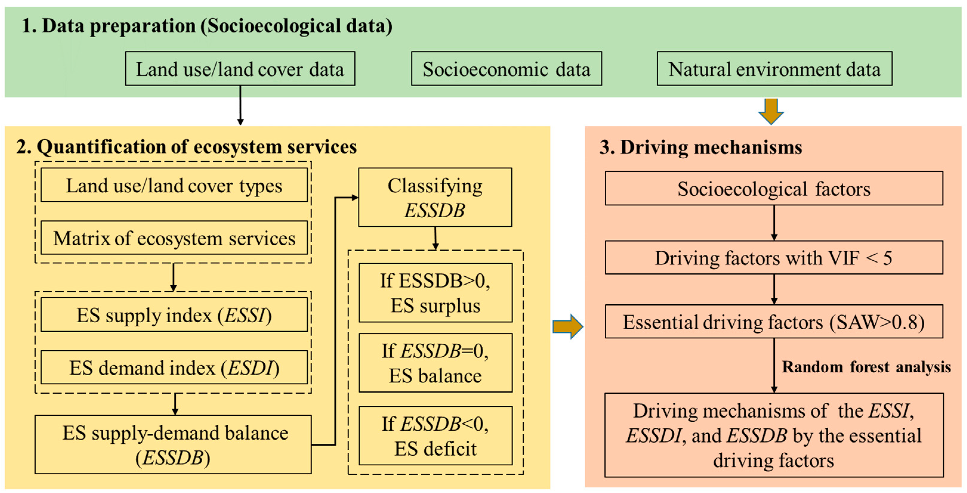
2.2. Theoretical Framework

This study consists of the following sections (Figure 2). First, LULC data, socioeconomic data and natural environmental data were collected and processed to ensure data consistency. Second, the ES supply and demand were calculated using the matrix of ESs, and the distribution characteristics of the ESs (including supply, demand, and supply–demand balance) were identified. Finally, we quantified the influence of the socioecological factors on the ESs, and explained the response processes and the driving mechanisms of the ESs by the socioecological factors using random forest analysis.

2.3. Data Preparation

The data used in this study included land use data, socioeconomic data and natural environmental data (Table 1). The same spatial resolution and projected coordinate system were used for all the data to ensure data consistency. The data sources used in this study are as follows:
(1) Land use/land cover (LULC) data at a 1 km resolution in 2020 were collected from the Resources and Environmental Science and Data Center Sciences (RESDC) at the Chinese Academy of Sciences (http://www.resdc.cn, accessed on 15 July 2023). These data are commonly used for research on land use changes and ecosystem services [17,19,48]. Six land use classes (cropland (CL), woodland (WL), grassland (GL), water body (WB), built-up land (BL), and unused land (UL)) with 23 subclasses were identified in the YREB (Figure S1 in the Supplementary Materials). This classification followed the LULC data classification standard of the Chinese Academy of Sciences [31]. The proportions of the six land use classes were also calculated.
(2) Socioeconomic data, including gross domestic product (GDP), per capita GDP (pGDP), total population (POP), population density (POPd) and urbanization rate (UR, proportion of urban population), were obtained from the statistical yearbooks of counties and districts of the YREB in 2021. The nighttime light index (NLI) was available at the RESDC.
(3) Natural environmental data include a digital elevation model (DEM), slope, annual average precipitation (PRE), annual average temperature (TEM), annual average evaporation (EVP), and normalized difference vegetation index (NDVI) data. DEMs were generated based on the latest SRTM Version 4.1 data, which were available at the RESDC. The slope dataset was created from DEM data with spatial analyst tools in ArcGIS 10.2 software (Environmental Systems Research Institute, Redlands, CA, USA). Meteorological data (PRE, TEM and EVP) were also downloaded free from the RESDC. The NDVI was extracted from the MODIS13Q1 products. The treatment method was in accordance with that used by Xiang et al. [48].

2.4. Quantification of Ecosystem Services

The ES supply and demand were evaluated using the assessment program proposed by Burkhard et al. [3], who established two matrices covering 44 CORINE LULC types and 22 ES supply/demand capacities. Therefore, we modified Burkhard’s matrices by linking similar LULC types between the CORINE land cover and the LULC used in this study according to their properties. Accordingly, referring to these matrices and to the LULC data used in this study, we screened 23 land use types and 22 ES categories. An ES supply matrix (Figure S2) and an ES demand matrix (Figure S3) were generated to assess the ES supply and demand in the YREB. Every intersection of LULC types and ESs in Figures S2 and S3 was scored from 0 (no supply or demand) to 5 (very high supply or demand), which indicated the ES supply capacities or the demand capacities for each LULC type [3,7,49].
Therefore, the ES supply index (ESSI) and the ES demand index (ESDI) can be calculated by the following formulas:
E S S I = j = 1 m i = 1 n A i × S C i j / i = 1 n A i
E S D I = j = 1 m i = 1 n A i × D C i j / i = 1 n A i
where SCij and DCij are the ES supply matrix and ES demand matrix of the j-th ecosystem services category of the i-th LULC type, respectively; Ai is the area (km2) of the i-th LULC type; n is the number of LULC types in this study (n = 1, 2, 3, …, 23); and m is the number of ES categories in this study (m = 1, 2, 3, …, 22). The results of the ESSI and ESDI at the county level were calculated using the “Zonal Statistics as Table” tool in ArcGIS 10.2 [7,29].
The ES supply–demand balance (ESSDB) at the county level was assessed using the following equation:
E S S D B k = E S S I k E S D I k ,     > 0 ,   E S   s u r p l u s     = 0 ,   E S   b a l a n c e < 0 ,   E S   d e f i c i t
where ESSDBk, ESSIk and ESDIk are the ES supply–demand balance, the ES supply index and the ES demand index of the kth county in the YREB, respectively. ESSDBk > 0 and ESSDBk < 0 represent a state of ES surplus and ES deficit, respectively, while ESSDBk = 0 indicates a state of ES balance.

2.5. Mechanisms Driving Ecosystem Services

2.5.1. Driving Factor Selection

Both natural conditions and anthropogenic activities can influence ES supply and demand, and further affect the ES supply–demand balance [25,50,51]. According to the relevant literature [52,53,54] and the availability of county-level data, 16 potential socioecological factors were selected to estimate their impact on the ES supply, demand and supply–demand balance.
A variance inflation factor (VIF) with a threshold value of 5 was used to decrease the effects of multicollinearity [55,56]. The vegan package (Version 2.5-7) [57] in R [58] was used to calculate the multicollinearity of the factors. Moreover, to reduce the dimensionality of the dataset while preserving the most information, the factors with a VIF < 5 were further eliminated according to the sum of their Akaike weights (SAW) with a threshold value of 0.8, which could be calculated in the package glmulti (Version 1.0.8) in R. If the SAW is greater than 0.8, this parameter was considered an essential driver in explaining the deviance in the ESs [59,60]. Essential drivers are regarded as good predictors of response variables without the need to refer to other variables [60].

2.5.2. Random Forest Analysis

A random forest model was applied in the randomForest package (Version 4.7-1.1) in R to identify the essential driving factors and their relative importance. The detailed steps are as follows [61]:
(1) The dataset was divided into a training set (70% of the dataset) and a test set (30% of the dataset);
(2) The accuracy of model calibration was assessed using the pseudo R2:
P s e u d o   R 2 = 1 M S E O O B V a r ( y )
where MSEOOB is the out-of-bag mean square error and Var(y) is the sample variance of the response variable y.
(3) The relative importance and marginal effects of essential driving factors on the ESSI, ESDI, and ESSDB in the YREB were quantified.
The relative importance of each driving factor to the ESSI, ESDI, and ESSDB was indicated by the percentage increase in the mean square error (%IncMSE) [28], which can be assessed using the following formula:
R I i = i n c M S E i / i = 1 f i n c M S E i
where RIi indicates the relative importance of factor i; incMSEi indicates the percentage of increase in the mean square error (%IncMSE) of factor i; and f is the number of selected socioecological drivers.
The marginal effects of selected socioecological factors on the ESSI, ESDI, and ESSDB were revealed by partial dependency, which can be assessed using the following formula [62]:
f ( x p ) = 1 s i = 1 s f ( x p , x C ( i ) )
where f(xp) is the predicated value of the ESSI, ESDI, or ESSDB; xp is the socioecological factor for which partial dependence is sought; xc(i) is the other socioecological factor in the dataset; and s is the number of counties and districts (1070 in this study). The marginal effect between the ESSI/ESDI/ESSDB and xp can be detected via Equation (6) by averaging over xc(i) [28].

3. Results

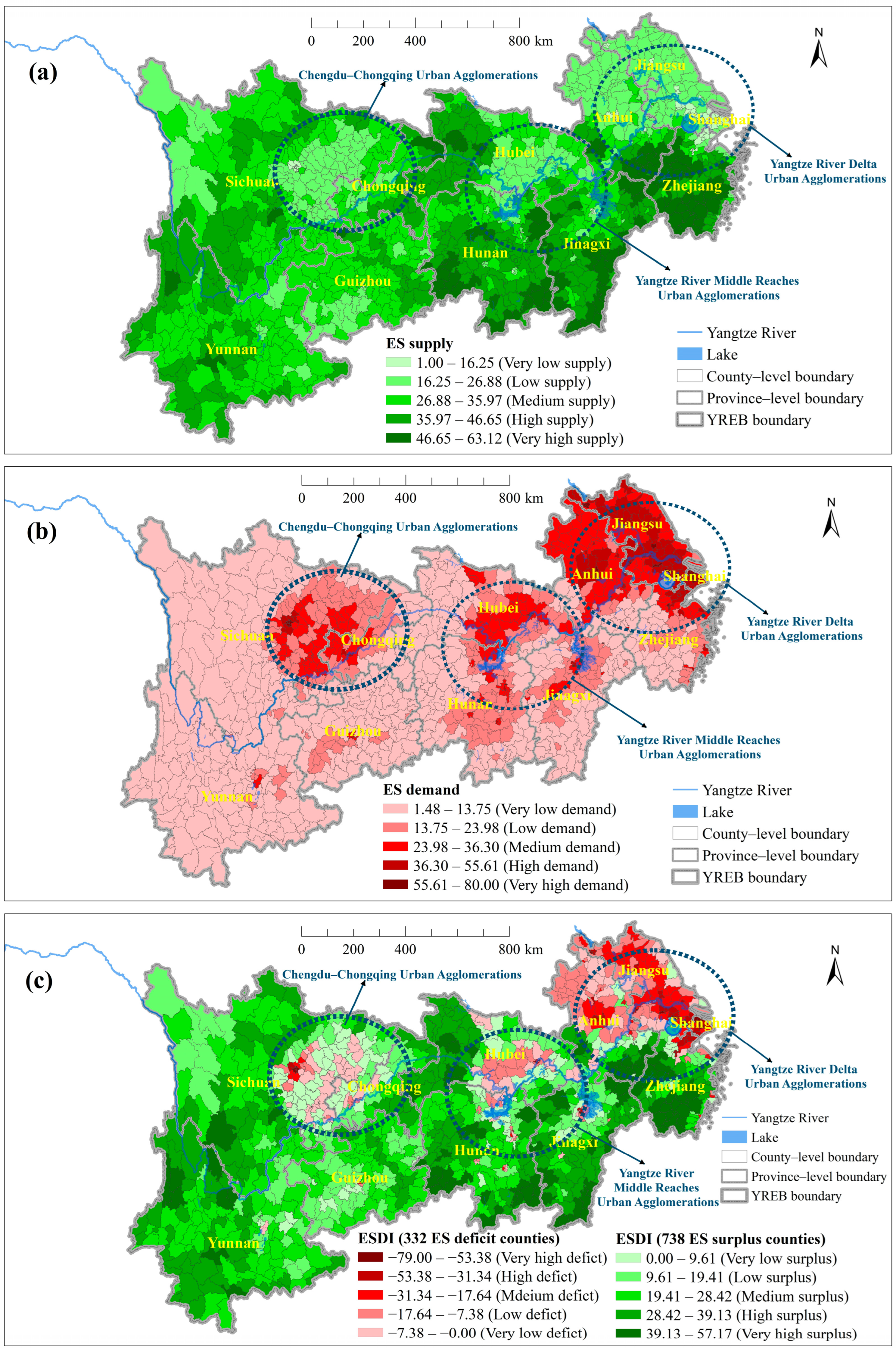
3.1. Spatial Distribution of Ecosystem Services in the YREB

The very high and high supply areas were mainly distributed in the southern parts of Zhejiang and Anhui Provinces and in the northwestern and southeastern areas of Jiangxi and Hunan Provinces (Figure 3a), where the woodlands are concentrated (Figure 1). Very low supply areas were primarily concentrated in the three national urban agglomerations, especially in Shanghai and most areas of Jiangsu and Anhui (Figure 3a), where built-up land and cropland were concentrated (Figure 1). In contrast, very high and high demand areas were predominantly distributed in three national urban agglomerations (Figure 3b) and very low demand areas were generally distributed in the upper and middle areas of the YREB, similar to the distribution of woodland (Figure 1) which was characterized by high elevation and steep slopes. In higher elevation areas with little interference from humans, the ESs were relatively greater; hence, the ES supply was greater than the demand.
Overall, the supply–demand balance of ESs featured a state of supply–demand surplus in the YREB. Moreover, at the county scale, the supply–demand balance of ESs presented an obvious spatial mismatch in that 332 (14.45% of the area) counties were distinguished by an ES deficit (Figure 3c). Similar to the distribution of ES demand, very high and high ES deficits were mainly located in the three national urban agglomerations. These agglomerations are suitable for living in and for industrial and agricultural development. The ES supply–demand balance was used to show the relationship between the ES supply and ES demand. A low capacity for ES supply and a high demand for ES may lead to ES deficits. For example, due to the high population density and high-intensity land use, the Yangtze River Delta Urban Agglomerations, especially Shanghai, Jiangsu and Anhui, had a low capacity for ES supply (Figure 3a and Figure S2) and a high demand for ES (Figure 3b and Figure S3), which was the main cause of the imbalance (deficit) between the supply and demand of ESs. The results also showed that deficit counties increased in area from upstream to downstream. In addition, the results indicated that the supply and demand for ESs varied by county.

3.2. Mechanisms Driving the ES Supply, Demand, and Supply–Demand Balance

3.2.1. Driving Factors

For the ES supply, seven essential driving factors (16 total factors) were identified according to the variance inflation factor (VIF) and the sum of their Akaike weights (SAW). Similarly, nine and eight essential driving factors were identified for ES demand and supply–demand balance, respectively (Table S1). Therefore, using these two indices (VIF and SAW), the number of driving factors greatly decreased (from 16 to 7/8/9, see Table S1 in the Supplementary Materials), while the simulation results maintained high accuracy in the random forest analysis (see Section 3.2.2).

3.2.2. Accuracy of the Random Forest Model

Random forest regression models were constructed to analyze the relationships between the socioecological factors and the ESSI, ESDI, and ESSDB in the YREB. A total of 1070 counties and districts were sampled for model construction. According to the random forest analysis, the pseudo R2 values of the test set for the ESSI, ESDI, and ESSDB were 0.84, 0.94, and 0.93, respectively. These results showed that essential driving factors could effectively explain the spatial variation in the ES supply, demand, and supply–demand balance. After model evaluation, relative importance plots were drawn to show the degree of influence of the essential driving factors on the ES supply, demand, and supply–demand balance. Furthermore, partial dependency plots of the essential driving factors (top five in terms of relative importance) were used to uncover the complex nonlinear relationships between the ES supply, demand, and supply–demand balance and the driving factors (Figure 4, Figure 5 and Figure 6).

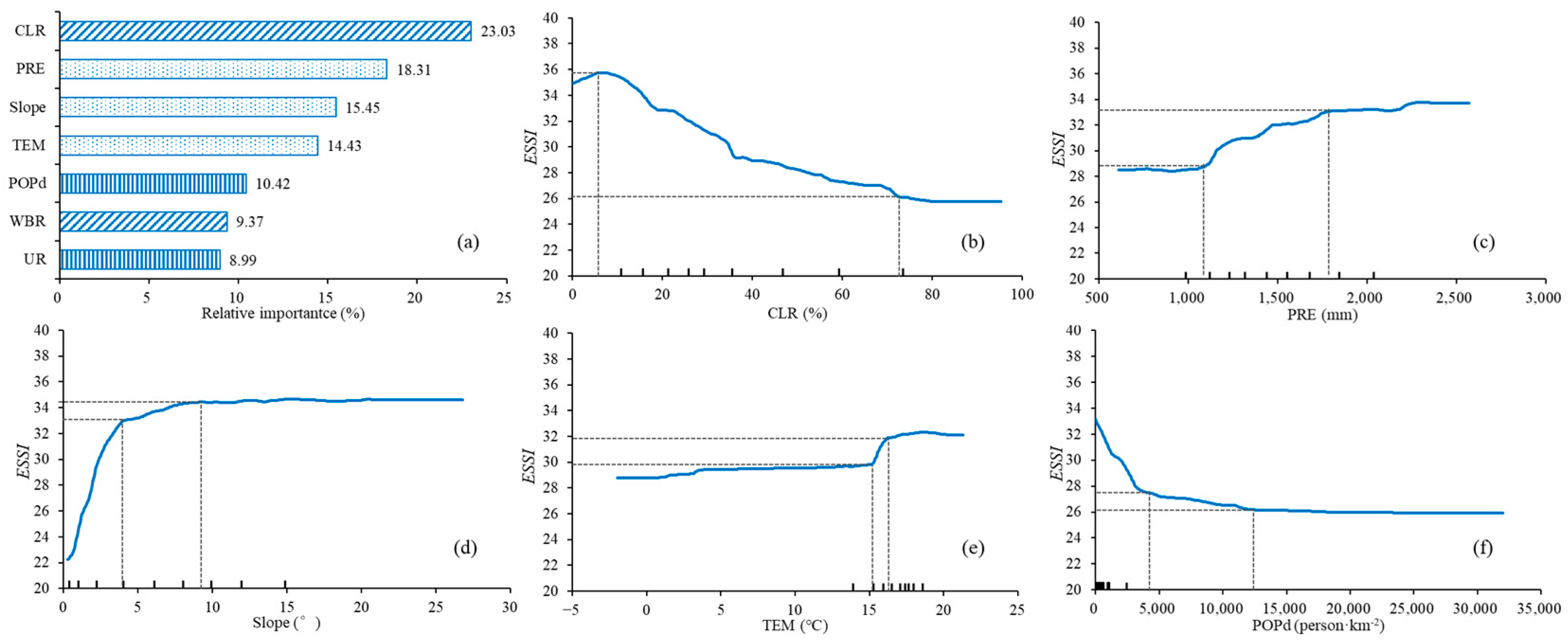
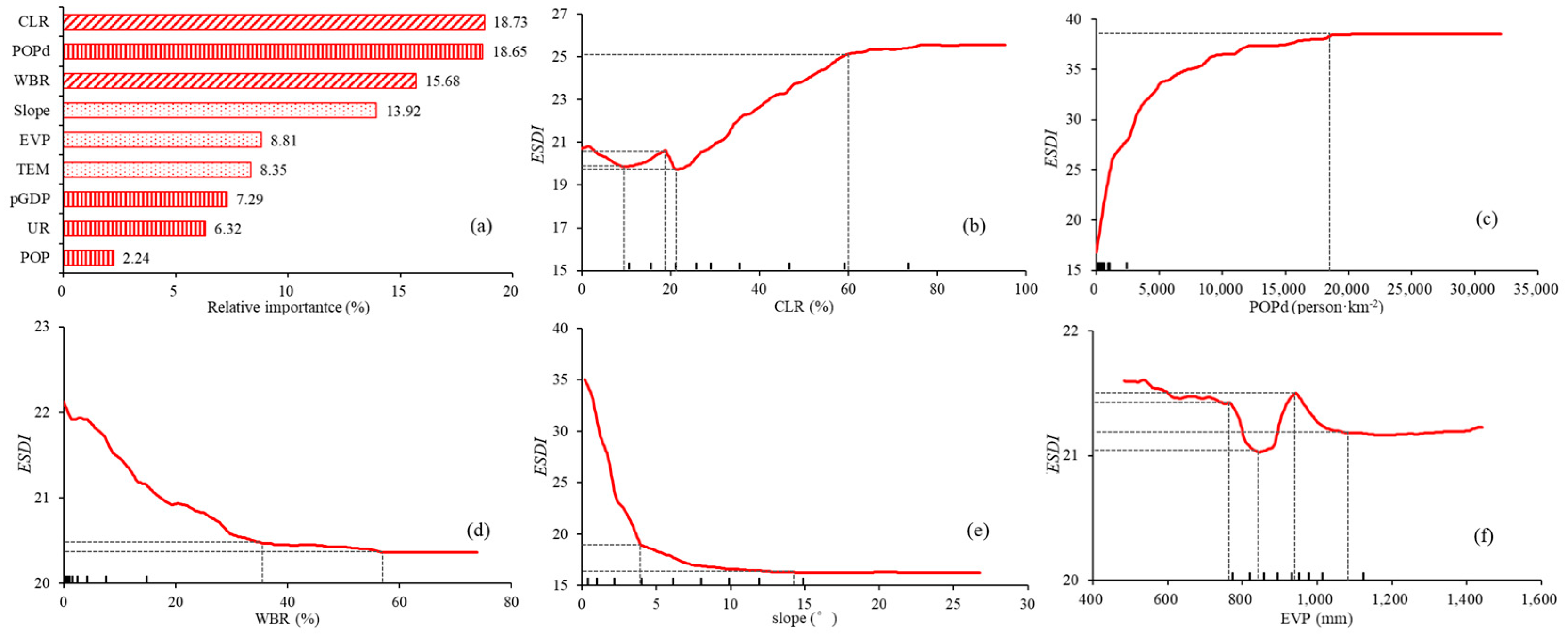
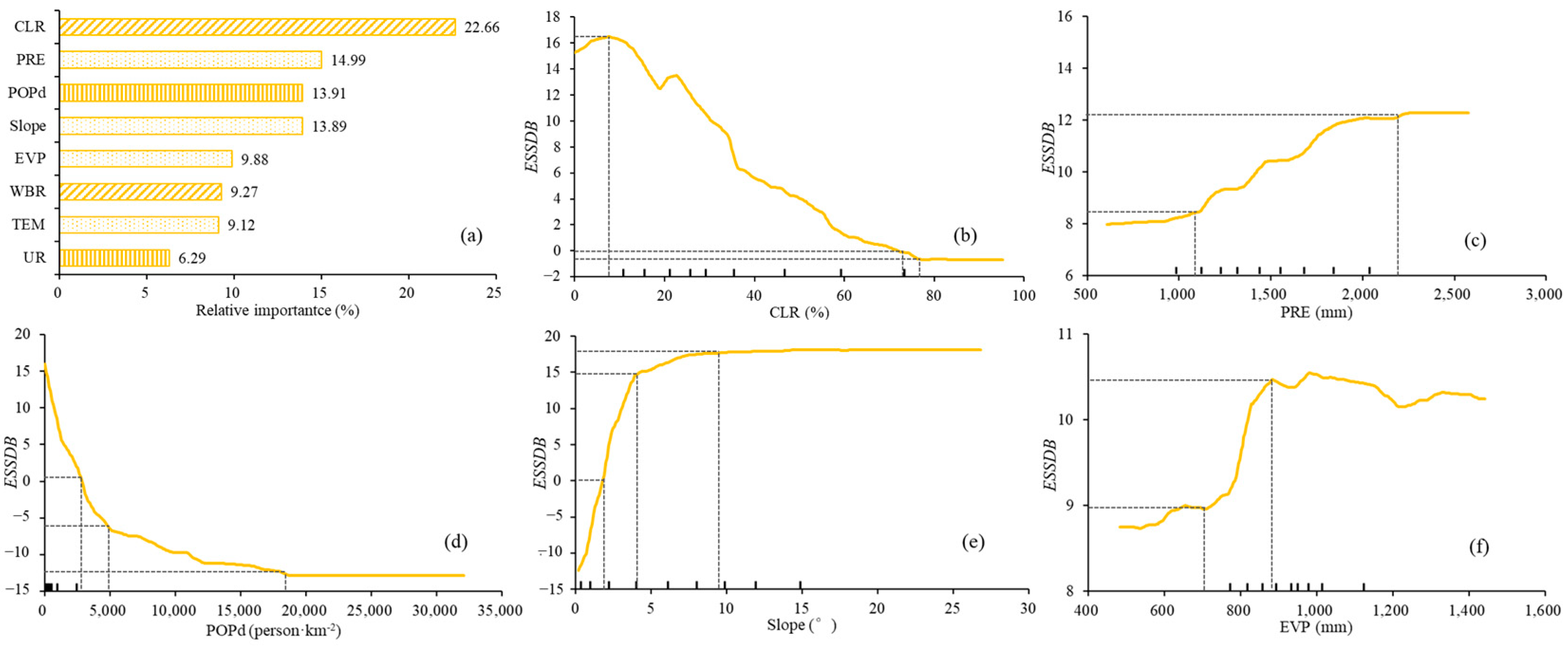
3.2.3. Socioecological Factors for the ES Supply, Demand, and Supply–Demand Balance

According to the relative importance rankings in Figure 4a, Figure 5a and Figure 6a, CLR and PRE were the two dominant factors influencing ESSI and ESSDB compared to the other factors, with a relative importance of 23.03% and 18.31% for ES supply and 22.66% and 14.99% for ESSDB, respectively. The importance of the other factors was ranked as 15.45% for slope, 14.43% for TEM, 10.42% for POPd, 9.37% for WBR, and 8.99% for UR for ESSI and 13.91% for POPd, 13.89% for slope, 9.88% for EVP, 9.27% for WBR, 9.12% for TEM, and 6.29% for UR for ESSDB. Obviously, the natural environmental factors had the greatest influence on the ESSI (48.19%) and the ESSDB (47.87%). Similarly, CLR had the greatest impact on the ESDI (18.73%), followed by POPd (18.65%), WBR (15.68%), and slope (13.92%), whereas EVP (8.81%), TEM (8.35%), pGDP (7.29%), UR (6.32%), and POP (2.24%) had minor influences. In addition, PRE had little effect on the ESDI. Therefore, the socioeconomic factors profoundly influenced the ESDI (34.51%).
The partial dependence plots show how each individual factor could impact the ESs (Figure 4, Figure 5 and Figure 6). Specifically, CLR demonstrated a nonlinear negative correlation with the ESSI, increasing slightly when CLR was below 7%, sharply decreasing between 7 and 75%, and slightly changing when CLR exceeded 75% (Figure 4b and Figure 6b). Similarly, with increasing POPd, the ESSI decreased significantly when POPd was below 4000 person·km−2 and declined slightly between 4000 and 12,000 person·km−2, after which the curve flattened (Figure 4f). However, as the PRE, slope, and TEM increased, the ESSI increased accordingly (Figure 4c–e). Specifically, the ESSI initially maintained a stable state when the PRE was below 1100 mm, followed by a general increase when the PRE was between 1100 and 1800 mm, and finally a slow increase when the PRE exceeded 1800 mm. The ESSI increased sharply when the slope was less than 4° and slightly increased between 4 and 9°, after which the curve flattened. Moreover, the ESSI increased slightly when the TEM was less than 15.2 °C, rapidly increased between 15.2 and 16.7 °C, and changed slightly when the TEM was greater than 16.7 °C.
The influence of EVP on the ESSDB replaced that of TEM in the ESSI, becoming the main factor affecting ESSDB. The influences of the other four factors (CLR, PRE, slope, and POPd) on the ESSDB (Figure 5) were the same as those shown in Figure 4, with slight differences in their relative importance rankings. The marginal effects of the other four factors (including patterns and turning points; see Figure 5) were similar to those shown in Figure 4. Overall, the driving factors had similar influences on the ESSI and ESSDB.
Conversely, CLR exhibited a positive correlation with the ESDI, and there were several turning points in the partial dependence plots for the CLR and ESDI (Figure 5b). Specifically, the influence declined slightly when the CLR was below 9.5% and between 19 and 22% and gradually increased between 9.5 and 19% and between 22 and 60%. When the CLR exceeded 60%, the ESDI remained stable. Similarly, with increasing POPd, the ESDI increased dramatically when POPd was below 18,500 person·km−2 and then maintained a stable state (Figure 5c). However, as the WBR, slope, and EVP increased, the ESDI generally decreased (Figure 5d–f). Specifically, the ESDI decreased sharply when the WBR was below 36% and decreased slightly between 36 and 55%, after which the curve flattened. The ESDI decreased sharply when the slope was less than 4°, slightly decreased between 4 and 14°, and then remained stable. Moreover, the ESDI decreased slightly when EVP was less than 850 mm, rapidly increased between 850 and 950 mm, and generally decreased when EVP was greater than 950 mm.

4. Discussion

4.1. Influence of Socioecological Factors on Ecosystem Services

In this study, a random forest regression model was used to explore the socioecological factors affecting the ES supply, demand, and supply–demand balance in the YREB. The simulation outcomes revealed that the natural environmental factors had the most significant influence on the ES supply, followed by the LULC and socioeconomic factors (Figure 4). In particular, PRE, TEM, and slope were the dominant factors influencing the ES supply, exhibiting a positive effect on the ES supply. These findings are similar to those of Fang et al. [63] in the Yangtze River Basin, Kang et al. [5] in the Yangtze River Delta and Wu et al. [49] in China. Moreover, this study revealed that CLR was the most important factor affecting the ES supply (Figure 4). Unlike our findings, previous studies have shown that the woodland ratio had the greatest influence on the ES supply [5,63]. A possible reason for their observation is that only several key ESs were selected for quantification, such as water yield, soil conservation, carbon storage, and water purification [63]. Woodlands generally have higher ES capacities and can contribute more benefits or products to humans (Figure S2). Therefore, stronger relationships between the woodland ratio and ES supply were detected in these studies.
In addition, this study revealed that socioeconomic factors markedly influenced the ES demand, and the impact of natural environmental factors on the ES demand became relatively limited. Socioeconomic factors are replacing natural environmental factors as the major factor influencing ES demand in the YREB. Notably, the importance of socioeconomic factors increased significantly; for example, the POPd was fifth in terms of the ES supply and second in in terms of the ES demand (Figure 4 and Figure 6), in which the ES demand exhibited a significant positive relationship with population density. Nevertheless, the results also showed that the CLR had the greatest positive effect on the relationships between ES demand (Figure 5). High-intensity agricultural activities and excessive population growth in the YREB have resulted in a remarkably high demand for ESs [64]. In contrast, where the slope is steeper, there are fewer industrial and agricultural activities, and the ES demand is lower [64]. This is the reason that ES demand declines as the slope increases.
Recent studies have shown that anthropogenic activities (such as industrialization, urbanization, and agricultural production) have gradually increased demand intensity and have decreased supply capacity and have further affected the ES supply–demand balance [16,28]. In general, ecologically intact land can provide greater ESs to ensure human well-being [3,7,63]. This study revealed that natural landscapes account for more than 65% of the total area in the study area; therefore, similar to the ES supply, natural environmental factors also play an important role in the ES supply–demand balance in the YREB (Figure 6). In particular, the slope and PRE exhibited a significant positive relationship with the ES supply–demand balance. Plains and areas with gentle slopes are the primary settlements for people, and steeper mountains with greater precipitation contribute more to the supply capacity of ESs [7,29].

4.2. Response Processes of Ecosystem Services to Socioecological Factors

Generally, the relationships between ESs and driving factors exhibit complex nonlinearity [6,28,38,39]. However, many studies have focused on the effects of individual and/or interactive socioecological factors on ESs [49,54,64]. Considering only the positive, negative or cumulative effects of key factors, we cannot assess the response processes of the ES supply–demand balance to multiple drivers. Hence, more studies should focus on the supply and demand of ESs, because systematic analyses of the supply and demand of ESs and their key drivers are critical for the development of effective policies to improve sustainable ecosystem management [16,54]. In addition, understanding these processes can provide useful guidance for ecological protection and ecological restoration programs to match ES supply and demand [6,28,65]. Therefore, the response processes of ESs (including supply, demand, and supply–demand balance) to key socioecological factors were identified in this study.
In general, three types of response processes could be summarized in this study. First, with increasing driving factors, the ESs decreased logarithmically. For example, with increasing POPd, the ES supply and supply–demand balance initially decreased sharply and then decreased slowly, followed by a stable state. Notably, when POPd was 2800 person·km−2, the ESSDB reached a state of ES balance (ESSDB = 0) (Figure 6d). A similar response process was found between the CLR and the ES supply and supply–demand balance, with a turning point occurring at 72% where the ES supply and demand balance was achieved. However, it should be noted that when the CLR was less than 7.0%, the ES supply and supply–demand balance increased slowly. This result means that a small amount of cropland reclamation can promote the balance of ES supply and demand. The possible reason is that cropland interspersed with woodland could increase landscape diversity and further improve the ES supply [66]. A similar result is shown in Figure 4b. In addition, this study also revealed that the ES demand decreased logarithmically with increasing slope and WBR.
Second, as the values of socioecological factors increased, the ESs increased logarithmically. For example, the ES supply and supply–demand balance changed sharply when the slope was below 4°, declined generally between 4 and 9°, and then remained stable, with a turning point occurring at 1.8° where the ESSDB reached a state of balance. Therefore, counties with a mean slope less than 1.8° should be considered regional hotspots of ES deficit. Especially in northern Jiangsu, Anhui, and Hunan and southern Hubei areas, the dominant land use type is cropland (Figures S4 and S5). As the cropland area expanded, the supply capacity of ESs decreased (Figure 4b) while the demand continued to increase (Figure 5b), which eventually led to the continuous decline of ESSDB (Figure 6b). This finding is similar to that of Wu et al. [28]. Moreover, we also found that the ES demand increased logarithmically with increasing POPd and CLR.
Finally, with increasing socioecological factor values, the ESs exhibited an increasing fluctuating trend. For example, the ES supply initially increased slightly when the PRE > 1100 mm and then increased gradually when the PRE > 1800 mm, followed by a basically stable state. In addition, with increasing EVP, the ES demand initially declined gradually until EVP = 850 mm and then increased significantly until EVP = 950 mm, followed by a slow decrease. The patterns and turning points of the partial dependence plots for EVP and PRE were similar to those between the ES supply and supply–demand balance (Figure 4 and Figure 6). Therefore, in the southern parts of Anhui and Hubei and the northern parts of Hunan and Jiangxi, where precipitation (1100–1800 mm) is significantly greater than evaporation (700–900 mm), the ESSDB gradually increased (surplus state, Figure 6 and Figure S4).

4.3. Implications for Ecosystem Management

According to the results of this study, several management measures are recommended to regulate the relationships between the supply and demand of ESs. First, the Grain for Green policy should be prioritized in areas with ES deficits, which were found in the three national urban agglomerations (Figure 3c). The random forest analyses showed that the ES supply decreased and ES demand increased sharply when the CLR increased from 7 to 72%. Counties with CLR > 72% (Figure 6b), which are located in the northern part of Anhui and Jiangsu, the eastern part of Sichuan, and the southern part of Hubei (Figure S5), should put more effort into promoting the implementation of the Grain for Green policy [54,66]. However, more importantly, in counties with less than 7% CLR, the implementation of the Grain for Green policy may not increase the ES supply; in contrast, it could reduce the ESSDB. Moreover, an excessively concentrated population could lead to a rapid reduction in the ES supply and an increase in the ES demand, eventually leading to ES deficits, especially when the population density exceeds 2800 persons·km−2. These regions are mainly distributed in densely populated urban centers (Figure S5).
Second, ES deficit areas were concentrated in counties with average slopes less than 1.8°, such as Jiangsu, the northern part of Anhui and Hunan, and the southern part of Hubei. As the slope increased, the ES supply–demand balance trend increased sharply until the slope < 4° and then increased gradually until the slope < 9°, followed by a stable state (Figure 6e). In addition, the ES demand remained stable when the slope was greater than 14°. Therefore, these four turning points (1.8°, 4°, 9°, and 14°) could be recommended to modify the current slope grading standards of land use and management (i.e., 2°, 6°, 15°, and 25°) and the ecological restoration of engineered slopes in China [67]. Therefore, the Grain for Green policy should be implemented in counties with flat terrain (slope < 1.8°), where the loss of topsoil and its fertility after returning cropland to forests could be reduced. This policy may facilitate ecological restoration and significantly improve the ES supply and ease ES deficits [68,69,70]. This may explain why the average slope of urban built-up land has shown an increasing trend in recent decades in China [71]. Policymakers should design urban planning at relatively steep slopes to ease the pressure of the imbalance between supply and demand for ESs.
Finally, anthropogenic activities have been considered one of the dominant factors in the spatiotemporal changes in temperature and precipitation during the recent decades, and have profoundly affected ESs [72,73]. Therefore, this study analyzed the influence of climatic factors (e.g., PRE and EVP) on the ES supply, demand, and supply–demand balance. The results illustrated that the decrease in precipitation and the increase in temperature and evaporation would promote an imbalance in the supply and demand of the ecosystem services, resulting in the emergence of ES deficits, especially when the PRE decreased from 2250 mm to 1100 mm (Figure 6c). At this time, water resource supplementation could increase the ES supply and decrease the ES deficit. Therefore, it is necessary to recharge water resources from upper water-rich areas to regions with less precipitation [74,75].

4.4. Limitations and Future Work

Using the county-level administrative districts in the YREB as research units, this study carried out a comprehensive analysis of the spatial distribution characteristics and balance patterns of ES supply and demand. Furthermore, this study also explored the response processes of ESs (including supply, demand, and supply–demand balance) to major driving factors. Although the results of this study could provide useful guidance for ecological protection and ecological restoration programs to match ES supply and demand, there are still some limitations.
First, the LULC-based matrix proposed by Burkhard et al. [3], which assigns expert scores to corresponding LULC types, was used to assess the ES supply, demand, and supply–demand balance in the YREB. This method assumed that the individual capacity for ES supply and demand (expert score) did not vary within a LULC type, although variations are likely [3,7,15]. A sensitivity analysis was applied to detect whether ES capacity is a robust proxy for LULC, and the results showed that the ES supply and demand were relatively inelastic with respect to changes in the ES capacities. This assessment of ES supply and demand in the Yangtze River Basin was relatively reliable [7]. Even so, a questionnaire-based survey of experts and stakeholders was recommended to obtain reasonable scores to modify the original LULC-based matrix [14,15]. Future studies should also consider modifying the LULC-based matrix with authoritative experts, experienced managers, and local residents. In addition, more complex assessment methods (such as the InVEST model and empirical formulas) [10,11,14] could be used to modify the LULC-based matrix.
Second, this study only analyzed the patterns, relationships, and driving forces of the ecosystem service supply and demand for one year, which cannot reflect spatiotemporal evolutionary characteristics. This is mostly because one of the main goals of this study is to propose a framework for identifying the relative importance and marginal effects of key driving factors on the ES supply, demand, and supply–demand balance. This study revealed that random forest models can be used to effectively identify the key driving factors and their driving processes at the county level. Future research can start from a long time series and a multi-spatial scale perspective to propose targeted policies for ecosystem enhancement [28,55,76]. Finally, this study did not separate the ES surplus areas and ES deficit areas when identifying the relative importance and marginal effects of key driving factors. Follow-up studies may account for the differences in the mechanisms driving the ES supply, demand, and supply–demand balance according to the socioecological factors that exist between ES surplus areas and ES deficit areas [13,77].

5. Conclusions

Based on the land use/land cover data of 2020 and combined with two ES matrices, this study analyzed the spatial distribution characteristics of ES supply, demand and supply–demand balance at the county level in the YREB. In addition, the response processes of the ES supply, demand and supply–demand balance to changes in socioecological factors were examined. The results revealed obvious spatial differences in the supply, demand and supply–demand balance in the YREB. The regions with a high ES supply were mainly located in the southeastern parts, while the high ES demand areas were mainly located in the three national urban agglomerations. Similarly, the ES deficit regions (332 of 1070 counties or 14.45% of the area) of the YREB were mainly concentrated in the three national urban agglomerations. We also found that natural environmental factors such as PRE and slope had a profound influence on the ES supply and supply–demand balance, while socioeconomic factors such as CLR and POPd had a significant impact on the ES demand. Notably, CLR ranked first among all the driving factors in terms of the ES supply (positive effect), demand (negative effect), and supply–demand balance (positive effect). Furthermore, our results indicated that the response processes of the ES supply, demand and supply–demand balance significantly differed with changes in the driving factors. Three types of response processes were identified in the YREB. First, the ESs decreased logarithmically with increasing driving factors. Second, the ESs increased logarithmically with increasing driving factors. Finally, ESs had an increasing fluctuating trend with increasing driving factors. Thus, turning points can be extracted from the three types of response processes, which should be focused on in future ecosystem restoration projects to ensure the success of these projects.

Supplementary Materials

The following supporting information can be downloaded at: https://www.mdpi.com/article/10.3390/land13060728/s1, Figure S1: The spatial distribution of the subclasses land use/land cover in the Yangtze River Economic Belt (YREB), China. Figure S2: Assessment matrix illustrating the capacities of different types for the land use/land cover classification system of China to supply ecosystem services. The values/colors indicate the following capacities: 0/White = no capacity; 1/Tzavorite green = very low capacity; 2/Light apple = low capacity; 3/Quetzel green = medium capacity; 4/Leaf green = high capacity; and 5/Fir green = very high capacity. Figure S3: Assessment matrix illustrating the demands for ecosystem services of humans living within the different types for the land use/land cover classification system of China. The values/colors indicate the following capacities: 0/White = no capacity; 1/Rose quartz = very low capacity; 2/Medium coral light = low capacity; 3/Poinsettia red = medium capacity; 4/Tuscan red = high capacity; and 5/Dark umber = very high capacity. Table S1: The selected driving factors for ES supply, demand, and supply–demand balance. Figure S4: Spatial distribution of chosen natural environment factors. (a) annual average precipitation, (b) annual average temperature, (c) annual average evaporation, (d) slope gradient. Figure S5: Spatial distribution of chosen LULC factors and socioeconomic factors. (a) cropland ratio, (b) water body ratio, (c) population density.

Author Contributions

Conceptualization, Z.Z. and Y.Y.; methodology, Z.Z., Y.Y. and F.F.; software, F.F., Q.J. and X.C.; validation, Z.Z., Q.J. and X.C.; formal analysis, Z.Z., Y.Y. and F.F.; investigation, Q.J. and X.C.; resources, Z.Z. and Y.Y.; data curation, Q.J. and X.C.; writing—original draft, Z.Z., Y.Y. and F.F.; writing—review and editing, Z.Z. and Y.Y.; visualization, Z.Z., Y.Y. and F.F.; supervision, Z.Z.; project administration, Z.Z. and Q.J.; funding acquisition, Z.Z. and F.F. All authors have read and agreed to the published version of the manuscript.

Funding

This work was supported by the Science & Technology Fundamental Resources Investigation Program (grant number 2023FY100101) and the National Natural Science Foundation of China (grant number 41977194).

Data Availability Statement

The original contributions presented in the study are included in the article, further inquiries can be directed to the corresponding author.

Acknowledgments

The authors thank all those who helped us complete this research.

Conflicts of Interest

The authors declare that they have no competing interests.

References

  1. Costanza, R.; d’Arge, R.; de Groot, R.; Farber, S.; Grasso, M.; Hannon, B.; Limburg, K.; Naeem, S.; O’Neill, R.V.; Paruelo, J.; et al. The Value of the World’s Ecosystem Services and Natural Capital. Nature 1997, 387, 253–260. [Google Scholar] [CrossRef]
  2. Costanza, R.; de Groot, R.; Braat, L.; Kubiszewski, I.; Fioramonti, L.; Sutton, P.; Farber, S.; Grasso, M. Twenty Years of Ecosystem Services: How far Have We Come and How far do We Still Need to Go? Ecosyst. Serv. 2017, 28, 1–16. [Google Scholar] [CrossRef]
  3. Burkhard, B.; Kroll, F.; Nedkov, S.; Muller, F. Mapping Ecosystem Service Supply, Demand and Budgets. Ecol. Indic. 2012, 21, 17–29. [Google Scholar] [CrossRef]
  4. Baró, F.; Palomo, I.; Zulian, G.; Vizcaino, P.; Haase, D.; Gómez-Baggethun, E. Mapping Ecosystem Service Capacity, Flow and Demand for Landscape and Urban Planning: A Case Study in the Barcelona Metropolitan Region. Land Use Policy 2016, 57, 405–417. [Google Scholar] [CrossRef]
  5. Kang, J.M.; Li, C.L.; Zhang, B.L.; Zhang, J.; Li, M.R.; Hu, Y.M. How Do Natural and Human Factors Influence Ecosystem Services Changing? A Case Study in Two Most Developed Regions of China. Ecol. Indic. 2023, 146, 109891. [Google Scholar] [CrossRef]
  6. Sun, Y.; Zhao, T.Y.; Cotella, G.; Liu, Y.S. Ecosystem Services Supply and Demand Mismatches and Effect Mechanisms in the Mixed Landscapes Context. Sci. Total Environ. 2023, 885, 163909. [Google Scholar] [CrossRef]
  7. Zhang, Z.M.; Gao, J.F.; Fan, X.Y.; Lan, Y.; Zhao, M.S. Response of Ecosystem Services to Socioeconomic Development in the Yangtze River Basin, China. Ecol. Indic. 2017, 72, 481–493. [Google Scholar] [CrossRef]
  8. Czúcz, B.; Arany, I.; Potschin-Young, M.; Bereczki, K.; Kertész, M.; Kiss, M.; Aszalós, R.; Haines-Young, R. Where Concepts Meet the Real World: A Systematic Review of Ecosystem Service Indicators and Their Classification Using CICES. Ecosyst. Serv. 2018, 29, 145–157. [Google Scholar] [CrossRef]
  9. Shen, J.S.; Li, S.C.; Wang, H.; Wu, S.Y.; Liang, Z.; Zhang, Y.T.; Wei, F.L.; Li, S.; Ma, L.; Wang, Y.Y.; et al. Understanding the Spatial Relationships and Drivers of Ecosystem Service Supply-demand Mismatches Towards Spatially-targeted Management of Social-ecological System. J. Clean. Prod. 2023, 406, 136882. [Google Scholar] [CrossRef]
  10. Liu, H.Y.; Xiao, W.F.; Zhu, J.H.; Zeng, L.X.; Li, Q. Urbanization Intensifies the Mismatch between the Supply and Demand of Regional Ecosystem Services: A Large-scale Case of the Yangtze River Economic Belt in China. Remote Sens. 2022, 14, 5147. [Google Scholar] [CrossRef]
  11. Hou, W.Y.; Hu, T.Z.; Yang, L.P.; Liu, X.C.; Zheng, X.Y.; Pan, H.Y.; Zhang, X.H.; Xiao, S.J.; Deng, S.H. Matching Ecosystem Services Supply and Demand in China’s Urban Agglomerations for Multiple-scale Management. J. Clean. Prod. 2023, 420, 138351. [Google Scholar] [CrossRef]
  12. Kong, L.; Wu, T.; Xiao, Y.; Xu, W.; Zhang, X.; Daily, G.C.; Ouyang, Z. Natural Capital Investments in China Undermined by Reclamation for Cropland. Nat. Ecol. Evol. 2023, 7, 1771–1777. [Google Scholar] [CrossRef] [PubMed]
  13. Wu, J.S.; Fan, X.N.; Li, K.Y.; Wu, Y.W. Assessment of Ecosystem Service Flow and Optimization of Spatial Pattern of Supply and Demand Matching in Pearl River Delta, China. Ecol. Indic. 2023, 153, 110452. [Google Scholar] [CrossRef]
  14. Zeng, J.; Cui, X.Y.; Chen, W.X.; Yao, X.W. Impact of Urban Expansion on the Supply-demand Balance of Ecosystem Services: An Analysis of Prefecture-level Cities in China. Environ. Impact. Assess. Rev. 2023, 99, 107003. [Google Scholar] [CrossRef]
  15. Cao, T.G.; Yi, Y.J.; Liu, H.X.; Xu, Q.; Yang, Z.F. The Relationship between Ecosystem Service Supply and Demand in Plain Areas Undergoing Urbanization: A Case Study of China’s Baiyangdian Basin. J. Environ. Manag. 2021, 289, 112492. [Google Scholar] [CrossRef]
  16. Li, J.Y.; Geneletti, D.; Wang, H.C. Understanding Supply-demand Mismatches in Ecosystem Services and Interactive Effects of Drivers to Support Spatial Planning in Tianjin Metropolis, China. Sci. Total Environ. 2023, 895, 165067. [Google Scholar] [CrossRef] [PubMed]
  17. Peng, J.; Wang, X.; Liu, Y.; Zhao, Y.; Xu, Z.; Zhao, M.; Qiu, S.; Wu, J. Urbanization Impact on the Supply-demand Budget of Ecosystem Services: Decoupling Analysis. Ecosyst. Serv. 2020, 44, 101139. [Google Scholar] [CrossRef]
  18. Bryan, B.A.; Ye, Y.Q.; Zhang, J.E.; Connor, J.D. Land-use Change Impacts on Ecosystem Services Value: Incorporating the Scarcity Effects of Supply and Demand Dynamics. Ecosyst. Serv. 2018, 32, 144–157. [Google Scholar] [CrossRef]
  19. Wang, X.Z.; Wu, J.Z.; Liu, Y.L.; Hai, X.Y.; Shanguan, Z.P.; Deng, L. Driving Factors of Ecosystem Services and Their Spatiotemporal Change Assessment Based on Land Use Types in the Loess Plateau. J. Environ. Manag. 2022, 311, 114835. [Google Scholar] [CrossRef]
  20. Schirpke, U.; Tasser, E.; Borsky, S.; Braun, M.; Eitzinger, J.; Gaube, V.; Getzner, M.; Glatzel, S.; Gschwantner, T.; Kirchner, M.; et al. Past and Future Impacts of Land-use Changes on Ecosystem Services in Austria. J. Environ. Manag. 2023, 345, 118728. [Google Scholar] [CrossRef]
  21. Li, J.; Jiang, H.; Bai, Y.; Alatalo, J.M.; Li, X.; Jiang, H.; Liu, G.; Xu, J. Indicators for Spatial-temporal Comparisons of Ecosystem Service Status Between Regions: A Case Study of the Taihu River Basin, China. Ecol. Indic. 2016, 60, 1008–1016. [Google Scholar] [CrossRef]
  22. Li, J.H. Identification of Ecosystem Services Supply and Demand and Driving Factors in Taihu Lake Basin. Environ. Sci. Pollut. Res. 2022, 29, 29735–29745. [Google Scholar] [CrossRef] [PubMed]
  23. Elliot, T.; Goldstein, B.; Gomez-Baggethun, E.; Proenca, V.; Rugani, B. Ecosystem Service Deficits of European Cities. Sci. Total Environ. 2022, 837, 155875. [Google Scholar] [CrossRef] [PubMed]
  24. Dabašinskas, G.; Sujetovienė, G. Spatial and Temporal Changes in Supply and Demand for Ecosystem Services in Response to Urbanization: A Case Study in Vilnius, Lithuania. Land 2024, 13, 454. [Google Scholar] [CrossRef]
  25. Wolff, S.; Schulp, C.J.E.; Verburg, P.H. Mapping Ecosystem Services Demand: A Review of Current Research and Future Perspectives. Ecol. Indic. 2015, 55, 159–171. [Google Scholar] [CrossRef]
  26. Zhang, J.; Duan, Y.; Zhou, S.; Huang, Y. Evaluation of the Effectiveness of Water Ecological Restoration Based on the Relationship between the Supply and Demand of Ecological Products—A Case Study of the Yellow River Delta. Land 2023, 12, 2093. [Google Scholar] [CrossRef]
  27. Xu, M.J.; Feng, Q.; Zhang, S.R.; Lv, M.; Duan, B.L. Ecosystem Services Supply-Demand Matching and Its Driving Factors: A Case Study of the Shanxi Section of the Yellow River Basin, China. Sustainability 2023, 15, 11016. [Google Scholar] [CrossRef]
  28. Wu, J.; Guo, X.; Zhu, Q.; Guo, J.X.; Han, Y.; Zhong, L.; Liu, S.Y. Threshold Effects and Supply-demand Ratios Should Be Considered in the Mechanisms Driving Ecosystem Services. Ecol. Indic. 2022, 142, 109281. [Google Scholar] [CrossRef]
  29. Yang, M.H.; Zhao, X.N.; Wu, P.T.; Hu, P.; Gao, X.D. Quantification and Spatially Explicit Driving Forces of the Incoordination Between Ecosystem Service Supply and Social Demand at a Regional Scale. Ecol. Indic. 2022, 137, 108764. [Google Scholar] [CrossRef]
  30. Zhai, T.; Ma, Y.; Fang, Y.; Chang, M.; Huang, L.; Ma, Z.; Li, L.; Zhao, C. Research on the Optimization of Urban Ecological Infrastructure Based on Ecosystem Service Supply, Demand, and Flow. Land 2024, 13, 208. [Google Scholar] [CrossRef]
  31. Peng, L.X.; Zhang, L.W.; Li, X.P.; Wang, Z.Z.; Wang, H.; Jiao, L. Spatial Expansion Effects on Urban Ecosystem Services Supply-Demand Mismatching in Guanzhong Plain Urban Agglomeration of China. J. Geogr. Sci. 2022, 325, 806–828. [Google Scholar] [CrossRef]
  32. Fedele, G.; Locatelli, B.; Djoudi, H.; Colloff, M.J. Reducing Risks by Transforming Landscapes: Cross-scale Effects of Land-use Changes on Ecosystem Services. PLoS ONE 2018, 13, e0195865. [Google Scholar] [CrossRef]
  33. Liu, J.; Wan, J.; Li, S.; Shen, Y.; Han, W.; Liu, G. Spatial–Temporal Pattern of Coordination between the Supply and Demand for Ecosystem Services in the Lhasa River Basin. Land 2024, 13, 510. [Google Scholar] [CrossRef]
  34. Castro, A.J.; Verburg, P.H.; Martín-López, B.; Garcia-Llorente, M.; Cabello, J.; Vaughn, C.C.; López, E. Ecosystem Service Trade-offs from Supply to Social Demand: A Landscape-scale Spatial Analysis. Landsc. Urban Plan. 2014, 132, 102–110. [Google Scholar] [CrossRef]
  35. Zhang, J.; Guo, W.; Cheng, C.J.; Tang, Z.Y.; Qi, L.H. Trade-offs and Driving Factors of Multiple Ecosystem Services and Bundles under Spatiotemporal Changes in the Danjiangkou Basin, China. Ecol. Indic. 2022, 144, 109550. [Google Scholar] [CrossRef]
  36. Zhao, Y.H.; Wang, N.; Luo, Y.H.; He, H.S.; Wu, L.; Wang, H.L.; Wang, Q.T.; Wu, J.S. Quantification of Ecosystem Services Supply-demand and the Impact of Demographic Change on Cultural Services in Shenzhen, China. J. Environ. Manag. 2022, 304, 114280. [Google Scholar] [CrossRef] [PubMed]
  37. He, G.Y.; Zhang, L.; Wei, X.J.; Jin, G. Scale Effects on the Supply-demand Mismatches of Ecosystem Services in Hubei Province, China. Ecol. Indic. 2023, 153, 110461. [Google Scholar] [CrossRef]
  38. Schwalm, C.R.; Anderegg, W.R.; Michalak, A.M.; Fisher, J.B.; Biondi, F.; Koch, G.; Litvak, M.; Ogle, K.; Shaw, J.D.; Wolf, A.; et al. Global Patterns of Drought Recovery. Nature 2017, 548, 202–205. [Google Scholar] [CrossRef]
  39. Ma, S.; Wang, L.J.; Jiang, J.; Chu, L.; Zhang, J.C. Threshold Effect of Ecosystem Services in Response to Climate Change and Vegetation Coverage Change in the Qinghai-Tibet Plateau Ecological Shelter. J. Clean. Prod. 2021, 318, 128592. [Google Scholar] [CrossRef]
  40. Li, D.L.; Cao, W.F.; Dou, Y.H.; Wu, S.Y.; Liu, J.G.; Li, S.C. Non-linear Effects of Natural and Anthropogenic Drivers on Ecosystem Services: Integrating Thresholds into Conservation Planning. J. Environ. Manag. 2022, 321, 116047. [Google Scholar] [CrossRef]
  41. Palacios-Agundez, I.; Onaindia, M.; Barraqueta, P.; Madariaga, I. Provisioning Ecosystem Services Supply and Demand: The Role of Landscape Management to Reinforce Supply and Promote Synergies with Other Ecosystem Services. Land Use Policy 2015, 47, 145–155. [Google Scholar] [CrossRef]
  42. Fan, Z.; Wang, X.B.; Zhang, H.J. Water Security Assessment and Driving Mechanism in the Ecosystem Service Flow Condition. Environ. Sci. Pollut. Res. 2023, 30, 104833–104851. [Google Scholar] [CrossRef] [PubMed]
  43. Liu, C.H.; Yan, X.L.; Han, Z.L.; Liu, Y.B.; Li, X.Z.; Li, X.Y.; Zhong, J.Q. Guiding and Constraining Reclamation for Coastal Zone Through Identification of Response Thresholds for Ecosystem Services Supply-demand Relationships. Land Degrad. Dev. 2024, 35, 1804–1817. [Google Scholar] [CrossRef]
  44. Bi, Y.Z.; Zheng, L.; Wang, Y.; Li, J.F.; Yang, H.; Zhang, B.W. Coupling Relationship Between Urbanization and Water-related Ecosystem Services in China’s Yangtze River Economic Belt and its Socio-ecological Driving Forces: A County-level Perspective. Ecol. Indic. 2023, 146, 109871. [Google Scholar] [CrossRef]
  45. Luo, Q.L.; Luo, Y.L.; Zhou, Q.F.; Song, Y. Does China’s Yangtze River Economic Belt Policy Impact on Local Ecosystem Services? Sci. Total Environ. 2019, 676, 231–241. [Google Scholar] [CrossRef]
  46. Lu, S.S.; Tang, X.; Guan, X.L.; Qin, F.; Liu, X.; Zhang, D.H. The Assessment of Forest Ecological Security and its Determining Indicators: A Case Study of the Yangtze River Economic Belt in China. J. Environ. Manag. 2020, 258, 110048. [Google Scholar] [CrossRef] [PubMed]
  47. National Bureau of Statistics of China. China Statistical Yearbook China; Statistics Press: Beijing, China, 2021. (In Chinese)
  48. Xiang, H.X.; Zhang, J.; Mao, D.H.; Wang, Z.M.; Qiu, Z.Q.; Yan, H.Q. Identifying Spatial Similarities and Mismatches Between Supply and Demand of Ecosystem Services for Sustainable Northeast China. Ecol. Indic. 2022, 134, 108501. [Google Scholar] [CrossRef]
  49. Wu, X.; Liu, S.L.; Zhao, S.; Hou, X.Y.; Xu, J.W.; Dong, S.K.; Liu, G.H. Quantification and Driving Force Analysis of Ecosystem Services Supply, Demand and Balance in China. Sci. Total Environ. 2019, 652, 1375–1386. [Google Scholar] [CrossRef] [PubMed]
  50. de Groot, R.S.; Alkemade, R.; Braat, L.; Hein, L.; Willemen, L. Challenges in Integrating the Concept of Ecosystem Services and Values in Landscape Planning, Management and Decision Making. Ecol. Complex. 2010, 7, 260–272. [Google Scholar] [CrossRef]
  51. Shaaban, M.; Schwartz, C.; Macpherson, J.; Piorr, A. A Conceptual Model Framework for Mapping, Analyzing and Managing Supply-demand Mismatches of Ecosystem Services in Agricultural Landscapes. Land 2021, 10, 131. [Google Scholar] [CrossRef]
  52. Lorilla, R.S.; Kalogirou, S.; Poirazidis, K.; Kefalas, G. Identifying Spatial Mismatches Between the Supply and Demand of Ecosystem Services to Achieve a Sustainable Management Regime in the Ionian Islands Western Greece. Land Use Policy 2019, 88, 104171. [Google Scholar] [CrossRef]
  53. Schirpke, U.; Candiago, S.; Vigl, L.E.; Jäger, H.; Labadini, A.; Marsoner, T.; Meisch, C.; Tasser, E.; Tappeiner, U. Integrating Supply, Flow and Demand to Enhance the Understanding of Interactions Among Multiple Ecosystem Services. Sci. Total Environ. 2019, 651, 928–941. [Google Scholar] [CrossRef] [PubMed]
  54. Wang, L.J.; Gong, J.W.; Ma, S.; Wu, S.; Zhang, X.M.; Jiang, J. Ecosystem Service Supply-demand and Socioecological Drivers at Different Spatial Scales in Zhejiang Province.; China. Ecol. Indic. 2022, 140, 109058. [Google Scholar] [CrossRef]
  55. Zuur, A.F.; Ieno, E.N.; Smith, G.M. Analysing Ecological Data, Statistics for Biology and Health; Springer: New York, NY, USA, 2007. [Google Scholar]
  56. Lemm, J.U.; Venohr, M.; Globevnik, L.; Stefanidis, K.; Panagopoulos, Y.; van Gils, J.; Posthuma, L.; Kristensen, P.; Feld, C.K.; Mahnkopf, J.; et al. Multiple Stressors Determine River Ecological Status at the European Scale: Towards an Integrated Understanding of River Status Deterioration. Glob. Chang. Biol. 2021, 27, 1962–1975. [Google Scholar] [CrossRef] [PubMed]
  57. Oksanen, J.; Blanchet, F.G.; Friendly, M.; Kindt, R.; Legendre, P.; McGlinn, D.; Minchin, P.R.; O’Hara, R.B.; Simpson, G.L.; Solymos, P.; et al. Vegan: Community Ecology Package Version 2.6-4. Available online: https://cran.r-project.org/web/packages/vegan/index.html (accessed on 23 December 2022).
  58. R Development Core Team. R: A Language and Environment for Statistical Computing; R Foundation for Statistical Computing: Vienna, Austria; Available online: https://www.r-project.org/ (accessed on 13 March 2015).
  59. Zhang, Z.M.; Gao, J.F.; Cai, Y.J. Effects of Land Use Characteristics, Physiochemical Variables, and River Connectivity on Fish Assemblages in a Lowland Basin. Sustainability 2023, 15, 15960. [Google Scholar] [CrossRef]
  60. Li, J.Q.; Bååth, E.; Pei, J.M.; Fang, C.M.; Nie, M. Temperature Adaptation of Soil Microbial Respiration in Alpine, Boreal and Tropical Soils: An Application of the Square Root Ratkowsky Model. Glob. Chang. Biol. 2021, 27, 1281–1292. [Google Scholar] [CrossRef] [PubMed]
  61. Breiman, L. Random Forests. Mach. Learn. 2001, 4, 5–32. [Google Scholar] [CrossRef]
  62. Friedman, J.H. Greedy Function Approximation: A Gradient Boosting Machine. Ann. Stat. 2001, 29, 1189–1232. [Google Scholar] [CrossRef]
  63. Fang, L.L.; Wang, L.C.; Chen, W.X.; Sun, J.; Cao, Q.; Wang, S.Q.; Wang, L.Z. Identifying the Impacts of Natural and Human Factors on Ecosystem Service in the Yangtze and Yellow River Basins. J. Clean. Prod. 2021, 314, 127995. [Google Scholar] [CrossRef]
  64. Wen, Y.L.; Li, H.B.; Zhang, X.L.; Li, T.Y. Ecosystem Services in Jiangsu Province: Changes in the Supply and Demand Patterns and its Influencing Factors. Front. Environ. Sci. 2022, 10, 931735. [Google Scholar] [CrossRef]
  65. Lin, Z.L.; Xu, H.Q.; Yao, X.; Yang, C.X.; Yang, L.J. Exploring the Relationship Between Thermal Environmental Factors and Land Surface Temperature of a “Furnace City” Based on Local Climate Zones. Build. Environ. 2023, 243, 110732. [Google Scholar] [CrossRef]
  66. Ma, S.; Wang, L.J.; Wang, H.Y.; Zhang, X.M.; Jiang, J. Spatial Heterogeneity of Ecosystem Services in Response to Landscape Patterns Under the Grain for Green Program: A Case-study in Kaihua County, China. Land Degrad. Dev. 2022, 3311, 1901–1916. [Google Scholar] [CrossRef]
  67. Shen, Y.F.; Li, Q.; Pei, X.J.; Wei, R.J.; Yang, B.M.; Lei, N.F.; Zhang, X.C.; Yin, D.Q.; Wang, S.J.; Tao, Q.Z. Ecological Restoration of Engineering Slopes in China—A Review. Sustainability 2023, 15, 5354. [Google Scholar] [CrossRef]
  68. Ouyang, Z.; Zheng, H.; Xiao, Y.; Polasky, S.; Liu, J.; Xu, W.; Wang, Q.; Zhang, L.; Xiao, Y.; Rao, E.M.; et al. Improvements in Ecosystem Services from Investments in Natural Capital. Science 2016, 352, 1455–1459. [Google Scholar] [CrossRef] [PubMed]
  69. Yu, Q.R.; Feng, C.C.; Xu, N.Y.; Guo, L.; Wang, D. Quantifying the Impact of Grain for Green Program on Ecosystem Service Management: A Case Study of Exibei Region, China. Int. J. Environ. Res. Public Health 2019, 16, 2311. [Google Scholar] [CrossRef] [PubMed]
  70. Cheng, Y.; Xu, H.H.; Chen, S.M.; Tang, Y.; Lan, Z.S.; Hou, G.L.; Jiang, Z.Y. Ecosystem Services Response to the Grain-for-Green Program and Urban Development in a Typical Karstland of Southwest China over a 20-year Period. Forests 2023, 148, 1637. [Google Scholar] [CrossRef]
  71. Shi, K.F.; Cui, Y.Z.; Liu, S.R.; Wu, Y.Z. Global Urban Land Expansion Tends to Be Slope Climbing: A Remotely Sensed Nighttime Light Approach. Earth’s Future 2023, 114, e2022EF003384. [Google Scholar] [CrossRef]
  72. Foley, J.A.; DeFries, R.; Asner, G.P.; Barford, C.; Bonan, G.; Carpenter, S.R.; Chapin, F.S.; Coe, M.T.; Daily, G.C.; Gibbs, H.K.; et al. Global Consequences of Land Use. Science 2005, 309, 570–574. [Google Scholar] [CrossRef] [PubMed]
  73. Gilman, J.; Wu, J.G. The Interactions among Landscape Pattern, Climate Change, and Ecosystem Services: Progress and Prospects. Reg. Environ. Chang. 2023, 23, 67. [Google Scholar] [CrossRef]
  74. Shi, Y.S.; Shi, D.H.; Zhou, L.L.; Fang, R.B. Identification of Ecosystem Services Supply and Demand Areas and Simulation of Ecosystem Service Flows in Shanghai. Ecol. Indic. 2020, 115, 106418. [Google Scholar] [CrossRef]
  75. Chen, Z.L.; Lin, J.Y.; Huang, J.L. Linking Ecosystem Service Flow to Water-related Ecological Security Pattern: A Methodological Approach Applied to a Coastal Province of China. J. Environ. Manag. 2023, 345, 118725. [Google Scholar] [CrossRef] [PubMed]
  76. Assis, J.C.; Hohlenwerger, C.; Metzger, J.P.; Rhodes, J.R.; Duarte, G.T.; Silva, R.A.D.; Boesing, A.L.; Prist, P.R.; Ribeiro, M.C. Linking Landscape Structure and Ecosystem Service Flow. Ecosyst. Serv. 2023, 62, 101535. [Google Scholar] [CrossRef]
  77. Wang, J.; Zhai, T.L.; Lin, Y.F.; Kong, X.S.; He, T. Spatial Imbalance and Changes in Supply and Demand of Ecosystem Services in China. Sci. Total Environ. 2019, 657, 781–791. [Google Scholar] [CrossRef] [PubMed]
Figure 1. The Yangtze River Economic Belt’s location (a), topography (b) and land use/land cover (c).
Land 13 00728 g001
Figure 2. Theoretical framework. VIF: variance inflation factor and SAW: sum of Akaike weights. Bold indicates the main contents and method of this study. The color of the background box is used to distinguish the specific contents contained in each main contents. The black arrow indicates the technical process. The orange arrow shows the relationship between the main contents. The italic symbols indicate the ES supply index, ES demand index, and ES supply–demand balance.
Land 13 00728 g002
Figure 3. Spatial distribution of the ES supply (a), demand (b), and balance (c) in the Yangtze River Economic Belt, China.
Land 13 00728 g003
Figure 4. Relative importance plots (a) and partial dependence plots (bf) of essential driving factors for the ESSI. Only the top five partial dependence plots for the essential driving factors were plotted. CLR: cropland ratio; PRE: annual average precipitation; Slope: slope gradient; TEM: annual average temperature; POPd: population density; WBR: water body ratio; UR: urbanization rate. Here, the natural environmental factors included the PRE, Slope, and TEM; the LULC factors included the CLR and WRB; and the socioeconomic factors included the POPd and UR.
Land 13 00728 g004
Figure 5. Relative importance plots (a) and partial dependence plots (bf) of essential driving factors for the ESDI. Only the top five partial dependence plots for the essential driving factors were plotted. CLR: cropland ratio; POPd: population density; WBR: water body ratio; Slope: slope gradient; EVP: annual average evaporation; TEM: annual average temperature; pGDP: per capita GDP; UR: urbanization rate; POP: total population. Here, the natural environmental factors included the Slope, EVP, and TEM; the LULC factors included the CLR and WRB; and the socioeconomic factors included the POPd, pGDP, UR, and POP.
Land 13 00728 g005
Figure 6. Relative importance plots (a) and partial dependence plots (bf) of essential driving factors for the ESSDB. Only the top five partial dependence plots for the essential driving factors were plotted. CLR: cropland ratio; PRE: annual average precipitation; POPd: population density; Slope: slope gradient; EVP: annual average evaporation; WBR: water body ratio; TEM: annual average temperature; UR: urbanization rate. Here, the natural environmental factors included the PRE, Slope, EVP, and TEM; the LULC factors included the CLR and WRB; and the socioeconomic factors included the POPd and UR.
Land 13 00728 g006
Table 1. List of data and data sources used in this study.
CategoryDataData TypeData Source
LULCLULC data in 2020Raster (1 km)http://www.resdc.cn, accessed on 15 July 2023
Socio economyGross domestic product (GDP) in 2020/Statistical yearbooks of counties and districts of the YREB in 2021
per capita GDP (pGDP) in 2020/
Total population (POP) in 2020/
Population density (POPd) in 2020/
Urbanization rate (UR) in 2020/
Nighttime-light index (NLI) in 2020Raster (1 km)http://data.tpdc.ac.cn, accessed on 15 July 2023
Natural environmentDigital elevation model (DEM) and SlopeRaster (1 km)http://www.resdc.cn, accessed on 20 July 2023
Annual average precipitation (PRE) in 2020Raster (1 km)
Annual average temperature (TEM) in 2020Raster (1 km)
Annual average evaporation (EVP) in 2020Raster (1 km)
Normalized difference vegetation index (NDVI) in 2020Raster (1 km)http://ladsweb.nascom.nasa.gov/, accessed on 20 July 2023
Disclaimer/Publisher’s Note: The statements, opinions and data contained in all publications are solely those of the individual author(s) and contributor(s) and not of MDPI and/or the editor(s). MDPI and/or the editor(s) disclaim responsibility for any injury to people or property resulting from any ideas, methods, instructions or products referred to in the content.

