Abstract
Urban heat island (UHI) mitigation and adaptation are urgent needs in a built environment, which requires us to search for sustainable solutions to limit the urban heat island effect and improve the energy efficiency of building envelopes. Among these solutions, vertical green structures (VGSs) have recently attracted significant attention for their potential to mitigate adverse effects, especially in densely built areas. This study presents a comprehensive data analysis of the microclimate of a living wall in Milan, Italy. Our aim was to evaluate this VGS’s performance in mitigating temperature increases caused by the UHI effect. In the literature, similar studies are limited to shorter monitoring periods (mostly in cooling seasons) and specific orientations (mostly facing south). However, the VGS presented in this case study here faces northwest and was continuously monitored for one calendar year. During this continuous in situ monitoring campaign, air temperature data from sensors either embedded in vegetation or exposed on a bare wall were collected and analysed over a whole calendar year, which is a novelty compared to the existing literature focused on VGSs due to the long duration. The findings indicate that the studied VGS has the ability to influence the outdoor microclimate depending on the season, the precipitation events, the wall exposure, the type of vegetation, and the vegetation’s phenological attributes. The analysis showed that the VGS consistently maintained cooler temperatures than the bare wall, with mean temperature differences ranging from 2.8 °C in autumn to 0.8 °C in spring through the winter. The vegetation acted as a natural insulator by reducing the air temperature during the hot summer and in early autumn, corresponding to the growing period of the vegetation. Thus, VGSs show potential to mitigate the global warming effect. These findings provide valuable insights on vegetation’s capability to act as a thermal regulator for sustainable urban planning and energy-efficient building design and retrofitting.
1. Introduction
1.1. Urban Heat Challenges and the Role of Vertical Green Structures
Climate change is a pressing issue that causes significant challenges to cities nowadays, with urban heat being one of the most crucial problems. Increasing global temperatures and changing weather patterns have led to an increase in extreme heat events in densely built urban areas in particular. These urban heat challenges are further exacerbated by the urban heat island effect (the UHI effect), which is a phenomenon that results from the absorption and re-emission of solar radiation by buildings, pavements, and other infrastructure during the day, leading to higher temperatures in cities [1]. The UHI effect is a big concern for the global population, as it contributes to negative impacts on many aspects such as public health, energy consumption, and the environment. The UHI effect is primarily driven by the rapid urbanisation and development of cities. An UHI can be also defined as an area under “a dome of stagnant warm air created by the concentration of buildings and infrastructure in urban areas” [2]. As cities expand and urbanise, natural surfaces such as vegetation are replaced with impervious surfaces that absorb and retain heat, leading to higher temperatures. In this context, building envelopes can provide opportunities to increase the amount of vegetative surfaces in urban areas.
Urban heat mitigation and adaptation are strategies and actions that aim to reduce the negative impacts of the UHI effect, as well as aiming to reduce extreme heat events in urban areas [3]. UHI mitigation strategies focus on lowering temperatures in urban environments through various means such as by increasing green spaces, using cool materials for buildings and pavements, implementing green surfaces, and enhancing urban ventilation. On the other hand, adaptation strategies include implementing heatwave early warning systems, providing cooling centres during heatwaves, designing buildings with heat-resilient features, and developing urban planning policies that consider heat resilience [4]. In this context, vertical green structures (VGSs), i.e., vertical surfaces covered with vegetation, offer a way to increase the greenery in urban areas and have recently become more attractive in compact built areas due to their independency from the horizontal plane. Due to novel materials, construction methods, and technological developments, VGSs have been increasing in variety. VGS typologies have been progressing from the traditional green façade (GF) with climbing plants to living walls (LWs) with more components and possible species to cultivate [5]. VGSs offer many simultaneous benefits, including the fact that they have a positive impact on climate-change-related challenges and contribute to its mitigation and adaptation: e.g., they contribute to carbon sequestration [6,7] by absorbing carbon dioxide (CO2) from the atmosphere and helping to locally reduce the concentration of greenhouse gases at a macroscale level. In addition, VGSs help to improve air quality by filtering pollutants and particulate matter from the atmosphere [8,9] because plants can absorb harmful gases and toxins, thus reducing their concentration in the urban environment and improving the overall air quality for residents. Finally, VGSs enhance urban biodiversity by providing habitats for various plant species and animals [10].
On an urban or a district scale, VGSs may contribute to mitigating urban heat and retained heat, thus making global warming and/or extreme hot-weather events less severe and less difficult to manage. VGSs, by shading buildings and surfaces, help to reduce the need for air conditioning, which lowers energy consumption levels [11,12]. On the scale of buildings or façades, VGSs can help to reduce energy needs for heating and cooling by providing thermal insulation [13]. The vegetation placed vertically acts as a barrier that reduces heat transfer through walls, in addition to horizontal surfaces, i.e., roofs. This can result in lowering energy demands with a consecutive reduction in greenhouse gas emissions associated with energy production.
Studies and publications on VGSs have increased in recent years, with changing approaches and interdisciplinary diversification. Thermal studies remain the most widespread theme, with observation campaigns of different durations [14]. Studies conducted in summer periods in the Mediterranean region have shown promising performances of VGSs in terms of their cooling effect. This is exemplified in the case study in [15], where a monitoring campaign was conducted for several parameters, i.e., exterior and interior (i.e., inside the building) surface temperatures, foliage temperature, and exterior and interior environment temperatures in four cardinal directions. The findings showed that the maximum daily temperature decrease on the outside of the east façade wall was about 5.7 °C, and this was 0.9 °C on the interior surface. Also, a recent study in the Mediterranean region evaluated the performance of a VGS after 4 weeks of monitoring and it reported maximum temperature differences of 8 °C and 27 °C between green and bare walls for the air and surface temperatures, respectively [16]. Another case [17] considered in addition the cloudiness of the sky as a condition during the test period. This study highlighted that a VGS enabled temperature reductions between 6.1 °C and 4 °C in comparison to a bare wall, on sunny and cloudy days, respectively. On the other hand, the VGS’s performance was lower in the autumn season according to similar experiments. Perini et al. [18] studied the effects of different VGSs, i.e., (1) a traditional green façade (exposed to the northwest), (2) an indirect green façade made with aluminium pots placed at several heights and steel frames (northeast), and (3) an LW with evergreen plant species cultivated in plastic boxes (west) on a building envelope in the Netherlands. They measured reductions of 1.2 °C, 2.7 °C, and 5 °C on the surfaces in the three cases, respectively.
Despite the general lack of studies conducted over continuous long-term monitoring periods, there are a few studies that measured the microclimatic parameters in a VGS during both winter and summer over the same calendar year. One of these few studies reports experimental research conducted on prototypes of VGSs located in five different sites in England [19]. These prototypes were monitored for their temperatures over a 1-year period. The five cases differed in their foliage thickness, orientation, and exposure. The results showed that, on average, the daily maximum temperature was 36% lower on the green façades than on bare ones. The vegetation reduced the daily maximum surface temperatures significantly, with the reduction ranging between 1.7 °C and 9.5 °C depending on the thickness of the vegetation cover varying from 10 cm to 45 cm, respectively. Another study [20] conducted in Berlin (Germany) showed that temperature differences under a green façade reached up to +3 °C during cold nights in winter due to the insulation effect, and up to −3 °C in summer due to the shading effect. During experimental research conducted in a laboratory using a direct GF and an LW, the authors of [21] found that the temperature differences between a bare wall and the direct green façade and the LW—after 8 h of heating, as in summer conditions—reached 1.7 °C and 8.4 °C, respectively. This significant variability in performances is due to the different components existing in each system. After 72 h, the measurement of the air temperature difference in the interior part was 2.1 °C.
1.2. Aims and Objectives
Based on the findings of the existing literature mentioned above, it can be said that a VGS is able to provide thermal regulation, especially in the summer season. However, there is a lack of existing studies that investigate the microclimate of a VGS by directly monitoring in situ the green structure throughout a typical calendar year. Hence, the monitoring campaign conducted in this work aims to evaluate the effects of having a VGS as a skin-like layer covering a building envelope. The temperature analysis is carried out across different temporal resolutions considering both a bare wall and a wall covered in vegetation to understand the microclimatic modifications caused by the vegetative layer over the 1 August 2021–31 July 2022 period. As a result, by evaluating the monitored air temperature anomalies between a sensor positioned on the reference bare (non-vegetated) wall and one embedded in the vegetated (VGS) wall, the temperature reduction capability of the VGS is assessed and compared with the data available in the literature. Finally, the VGS’s capability to mitigate the effects of climate change in a densely built environment, such as that of the Milan city centre, is investigated by analysing a long-term climatic dataset, taking advantage from the analysis of long-term climate reconstruction in the Milan city centre reported in [22]. The novelty of this study lies in (1) its comprehensive monitoring of the VGS’s performance over a single calendar year, which includes a method to reconstruct missed data and a detailed identification of stressful periods for the vegetation and optimal weeks during the growing season; (2) its assessment of temperature regulation potential during the calendar year in terms of climate change, as derived from comparisons made between monthly temperatures taken over different time periods, i.e., between a far-past reference period (1763–1792) obtained from the earliest records of the Milan temperature series, representative of the past climate, and the contemporary 2021–2022 monitored period.
2. Materials
2.1. Location and Climatic Conditions
The case study presented in this contribution was conducted in Milan, a mid-latitude city in Northern Italy’s inland plains with a humid subtropical climate corresponding to the Cfa Köppen–Geiger (KG) climate classification. Milan has hot, humid summers, with at least one month’s average temperature being above 22 °C; cold, foggy winters, with the coldest month averaging above 0 °C; and at least four months in the mid-seasons averaging above 10 °C [23].
Within this context, the study area considered in this contribution (Figure 1b,c) is in Piazza della Repubblica, 20, 20124 Milan, a district densely built as a business centre; the building hosting the outdoor VGS functions as a hotel named The Westin Palace, as shown in Figure 1. Figure 1a also shows the distances between the location of the monitored VGS in the city centre of Milan (light-green dot denotes The Westin Palace); the weather station installed by the Regional Agency for Protection and the Environment of the Lombardy region (ARPA, yellow dot), located at a distance of 1.7 km and used in this study to reconstruct the missing monitored data; and the Brera Astronomical Observatory weather station (orange dot), located at a distance of 1.3 km and used to assess the impact of climate change over the last 260 years.
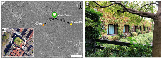
Figure 1.
(a) Locations of the sites used in this case study (including The Westin Palace) in Milan. Yellow dot: ARPA weather station (Juvara); orange dot: Brera Astronomical Observatory weather station. (b) Zoomed-in aerial image of the studied building: The Westin Palace. (c) Photograph of the VGS facing northwest (Ogut, O., 20 March 2022).

2.2. Building Characteristics, VGS Characteristics, and Cultivated Species
The vegetated façade (Figure 1c) is faced to the northwest and has a total dimension of 23 m2. It consists of four different species, i.e., Czakor, also known as big-root cranesbill (Geranium macrorrhizum); sneezewort, or “Perry’s White” (Achilea pitarmica); obsidian (Heuchera micrantha); and star jasmine (Trachelospermum jasminoedes). The features of these plant species are reported in Table 1 below.

Table 1.
Characteristics of the plant species cultivated in this VGS case study.
Table 1.
Characteristics of the plant species cultivated in this VGS case study.
| Scientific Name | Geranium macrorrhizum | Achilea pitarmica | Heuchera micrantha | Trachelospermum jasminoedes |
|---|---|---|---|---|
| Picture |  |  |  |  |
| Common name(s) | Czakor, big-root cranesbill | Sneezewort, Perry’s White | Obsidian, crevice alumroot | Star jasmine |
| Native area | SE Alps, Balkans | Europe, W Asia | W N America, British Columbia | E and SE Asia |
| Water | X | XX | X | X |
| Light | XXX | XX-XXX | XX | XX-XXX |
| Blooming months | 6–10 | 6–9 | 6–7 | 6–8 |
| Growth and form categories | H, D, E, T | H, D, E, T | H, D, T | W, E |
Notes: The capital letters in the “Native area” row stand for the acronyms of cardinal directions. X, XX, XXX represent low, medium, high levels for the described requirements. The blooming periods refer to months from 1 to 12, indicating January to December. Plants: H = herbaceous, W = woody, D = deciduous, E = evergreen, T = tender.
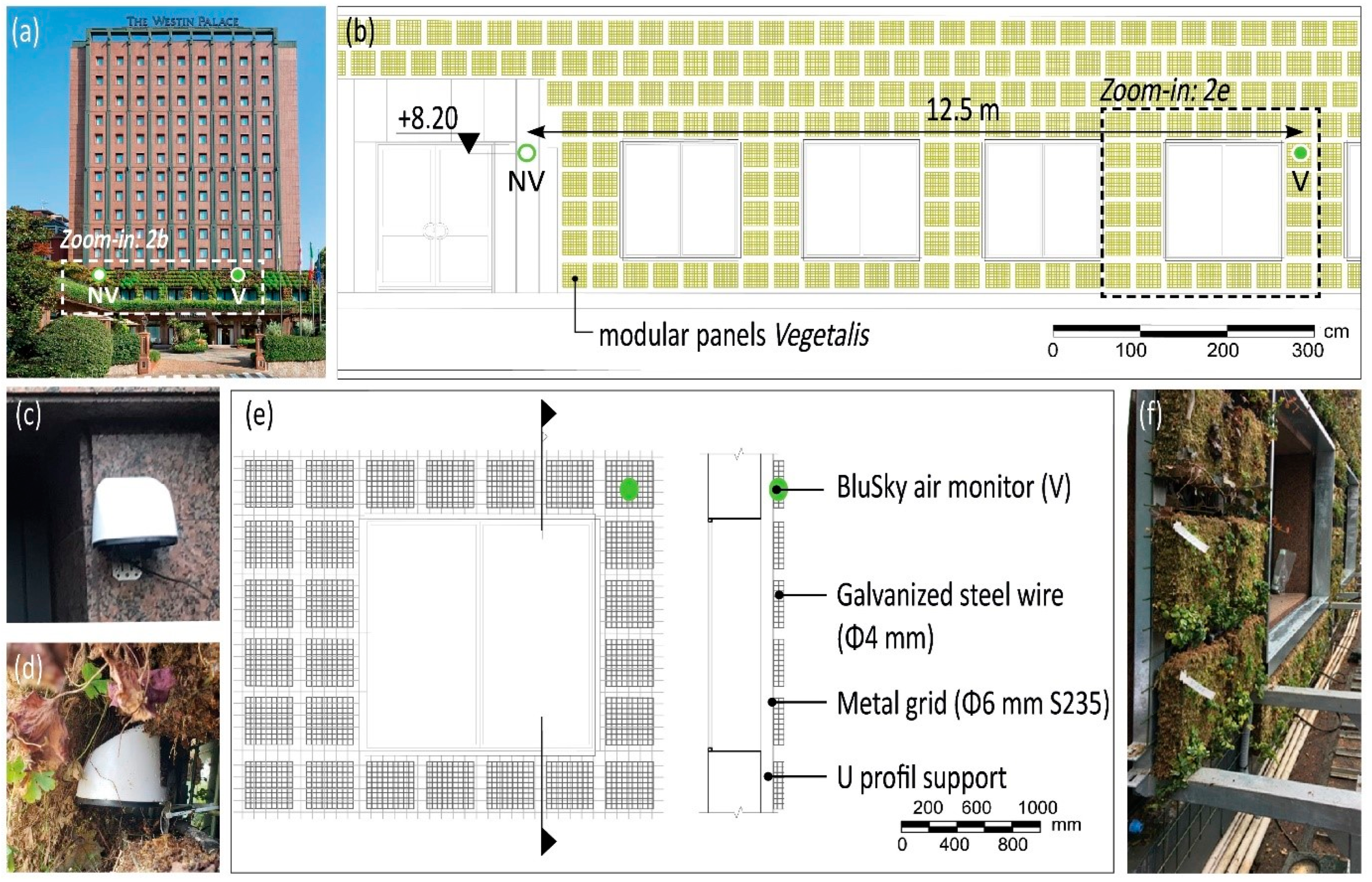
To be specific, this VGS belongs to the LW typology [5] that has a high number of components and a high level of technology; the system was developed by Peverelli srl Giardini e Paesaggi d’autore [24]. It comprises modular box frames (variable dimensions based on specific requirements) made of galvanised steel wire, assembled to the anchoring structure (i.e., a steel grid) by using metal hooks, as shown in Figure 2e. The hooks are attached to the original façade using dowels and screws. Inside the boxes, modular panels called Vegetalis are used. These are made of foam-based growing media using vegetal and natural substrates consisting of an aquatic foam (Figure 2f). Finally, the VGS is equipped with dispensers that allow the moisture in the soil to be adjusted to provide optimal conditions for the growing medium consisting of Sphagnum sp. moss.
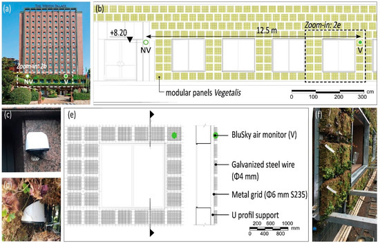
Figure 2.
(a) Elevation of The Westin Palace hotel façade. (b) Zoom-in showing the details of the monitored part of the façade. (c,d) BlueSky™ Air Quality Monitors (Thermo-Systems Engineering Co., USA), (c) positioned on a bare surface (NV wall) and (d) positioned on the VGS surface (V wall). (e) Section of the LW system: the ±0.00 level is considered the entrance/ground-floor level. (f) Modular panel system with growing media.
2.3. Monitoring Setup
Two BlueSky™ Air Quality Monitors, laser-based particle instruments [25] produced by TSI Incorporated (Thermo-Systems Engineering Co., USA), were installed on the façade of the hotel (Figure 2a,b): one in contact with the bare surface (i.e., the NV wall) (Figure 2c) and the other one embedded into the LW system (i.e., the V wall) (Figure 2d). The selection of the locations of these instruments was conditioned by the availability of access points to the internet and electricity and the availability of an easy-to-inspect position in case of complications, while at the same time keeping the visual impact as low as possible, as requested by the building owner. The BlueSky instruments measured particulate matter (PM) mass concentrations in micrograms (one-millionth of a gram) per cubic meter of air (μg/m3), as well as providing real-time temperature measurements in °C and relative humidity in % simultaneously. The measurements of the parameters were set to occur continuously every 15 min. The monitoring campaign started on 1 August 2021, and the analysed data presented here cover one calendar year until 31 July 2022.
3. Methodology
The methodological approach of this study—based on in situ monitoring—is described in a scheme in Figure 3. The analysed datasets were collected from different sources, as highlighted with a colour code in Figure 1a (locations and distances of these data sources) and in Figure 3 (names of the datasets and stages in which they were used in this analysis). They were collected in the following ways:
- −
- Through a dedicated monitoring campaign conducted by the authors during the 2021–2022 period (green dots: BlueSky datasets) [25];
- −
- Through retrieving data from the nearby weather station of v. Juvara (yellow dots: ARPA datasets) installed by ARPA (the Regional Agency for Protection and the Environment of the Lombardy region) [26];
- −
- Through downloading data from the HISTALP database (Historical Instrumental Climatological Surface Time Series of the Greater Alpine Region) [27]. The HISTALP datasets refer to the long-term historical data collected at the weather station of the Brera Astronomical Observatory, a research centre of excellence of the National Institute of Astrophysics (INAF), located in Milan city centre (orange dots: HISTALP datasets—filled and void dots refer to HISTALP datasets for the near-past (NP, 1991–2020) and extremely far-past (EFP, 1763–1792) temporal ranges).
The data analysis consisted of several steps, which are visible in Figure 3 inside the white boxes, together with their interconnections (arrows in Figure 3) that are explained in the following section.
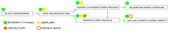
Figure 3.
Datasets and analysis steps followed during the study. Data sources are highlighted with a colour code and a short ID in the legend.
Figure 3.
Datasets and analysis steps followed during the study. Data sources are highlighted with a colour code and a short ID in the legend.

3.1. Data Reconstruction
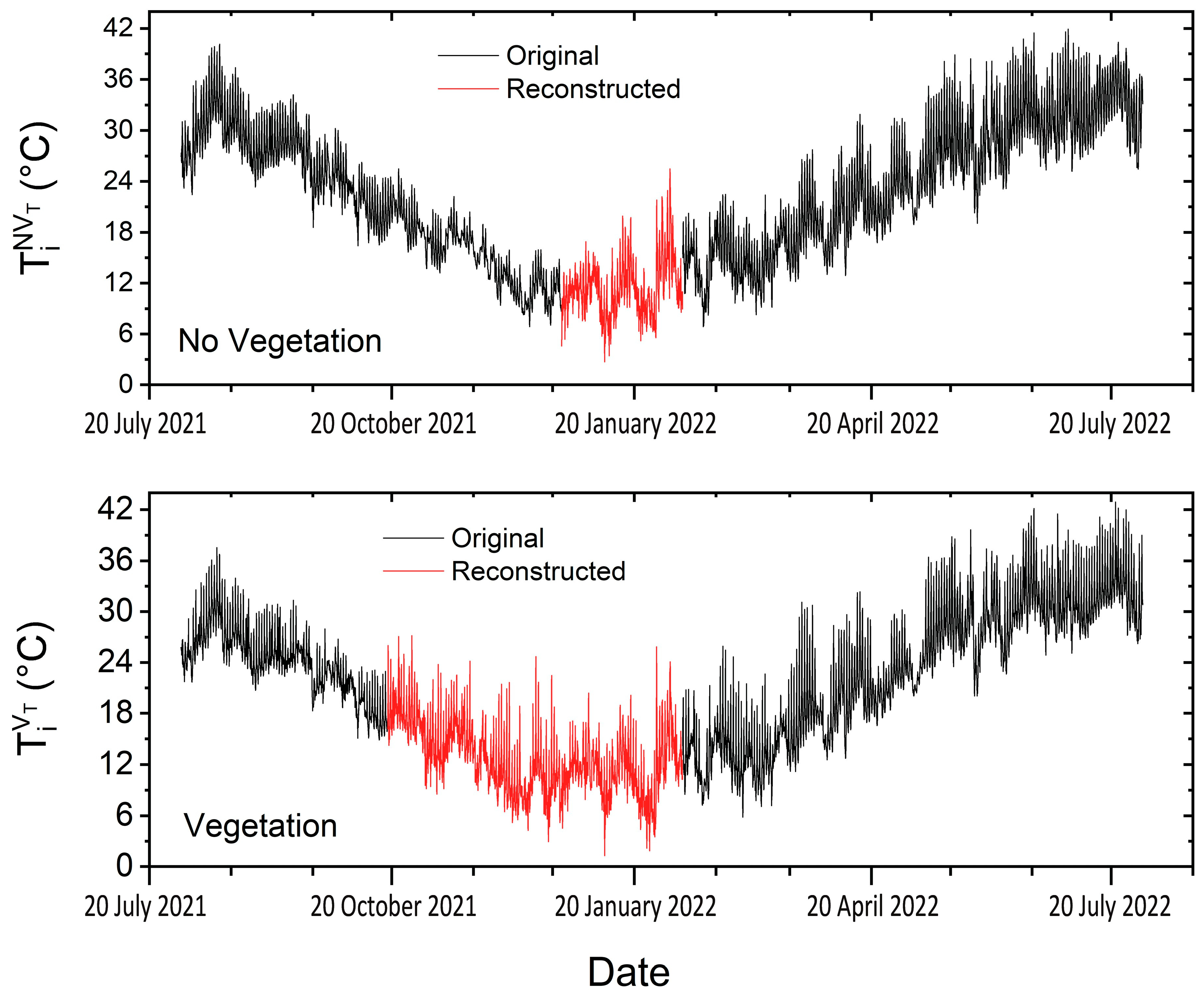
Due to the unstable Wi-Fi connection of the BlueSky devices, the data were downloaded by the authors from the micro-Secure Digital (micro-SD) cards mantled inside the monitors instead of using the Cloud. During the data retrieval, some issues were encountered that caused data losses. The main issue was that a power outage occurred. Since the devices relied on a continuous power source, the electrical disconnection resulted in data being lost during the monitoring period. The missing data spanned from 18 October 2021 to 7 February 2022 and from 23 December 2021 to 7 February 2022, for the monitors installed on the vegetated (V) and non-vegetated (NV) walls, respectively, as plotted in Figure 4 (red lines).
The ARPA time series (ART) allowed us to restore the completeness of the monitored VGS data by using a novel reconstruction method for missing data. The method here proposed calculates the mean daily thermal gradient in relation to the season (subscript S in the equations) using the following formula:
where is the mean hourly (H) temperature (T) in relation to the season S, and n refers to all of the i-th hourly data available for the same season (e.g., ). The average daily (subscript D) thermal gradients were calculated for the three datasets (i.e., the two monitored by the authors using the BlueSky equipment, i.e., VT and NVT, and the dataset retrieved by ARPA, i.e., ART) and for the seasons (∇) in which the data gap of VT and NVT occurred. The difference between the gradients (∇∇ and ∇∇) allowed us to evaluate the vegetation’s influence on the wall temperature in relation to the hourly air temperature data available from the ARPA weather station (ART), thus allowing us to reconstruct the missing data at an hourly resolution. The hourly reconstruction factor (HRF) that was added to the time series ART reconstructed the two-time series VT and NVT as follows:
3.2. Data Analysis
Once the raw data (i.e., comma-separated value (csv) files) for each week of the monitoring campaign, as recorded using the BlueSky instruments, were reconstructed (referred to as the complete database or dataset from now on) following the procedure described in Section 3.1, the data analysis started. To this aim, the complete dataset was divided into time features, i.e., year, season, month, day, and hours, to be able to calculate the maximum, minimum, and average values over different time windows with hourly (H subscript in the following equations) and daily resolution. These calculations were completed using the IF function of Microsoft Excel, which provides statistical values of cells that meet multiple criteria. The functions used for the hourly minimum, maximum, and average temperature values were the MINIFS, MAXIFS, and AVERAGEIFS functions, respectively, as reported below:
The range of each statistical measure (i.e., min, max, and average) included all of the measured temperature values. Once we had calculated , , and , depending on the temporal resolution selected in the analysis, the same Formulas (4)–(6) were used with different input data (in such a case, the subscript changes to the season, month, or day). As an example, to calculate daily statistics (i.e., min, max, and mean), hourly data were used as the input, while to calculate monthly statistics, daily data were used instead.
Table 2 reports the seasonal statistical measures of temperature differences between the non-vegetated (NV) and vegetated (V) walls. The results are categorised according to the day and night times, as well as in relation to no-rain days (NRDs) and rainy days (RDs). To build the table, the seasons were considered as meteorological seasons based on groupings of consecutive months, defined as follows: March, April, and May, standing for spring; June, July, and August, standing for summer; September, October, and November, standing for autumn; and December, January, and February, standing for winter. The day was considered to last from 8.00 to 19.00 and the night lasted from 20.00 to 7.00. Moreover, the rainy days in the monitoring period were those with precipitation higher than 1 mm. The no-rain days represented the others.
In addition to seasonal findings, smaller temporal windows were considered for further analyses. The impact of the VGS on modifying the temperature in proximity to the wall surface was analysed according to the anomaly between the reconstructed monitoring reference series described in the previous section:
where i is the i-th hourly mean measurement for the bare wall () or the vegetated wall ().
To better visualise the inter-weekly and weekly TAnomaly,VGS variability, and to illustrate the overall microclimatic conditions during the monitoring period of August 2021–June 2022, the running averages over time windows of 3 and 7 days were calculated and are presented in Figure 5a,b (top panel), respectively, together with precipitation values (millimetres, centre panel) and air temperature (°C, bottom panel) from the ARPA weather station. In connection with this analysis, the temperature monthly averages of the two V and NV monitored datasets over the 2021–2022 period allowed us to clearly observe in which period of the year (i.e., TAnomaly,VGS representative threshold value) the VGS has a higher potential cooling effect on the wall surface due to the optimal vegetative growth. This was calculated with Equations (8) and (9), below:
where is the monthly (subscript M) mean temperature of the monitored NV wall, with being that of the V wall, and n is the hourly T values in a specific month, ranging from 1 = January to 12 = December.
Three-day and seven-day VGS anomaly running averages larger than the identified TAnomaly,VGS representative threshold value after precipitation events highlighted an optimal vegetative growth of the VGS. The occurrence of such events is highlighted in Figure 5a,b and Figure 6 by the green background. Similarly, the second TAnomaly,VGS representative threshold occurring in conjunction with precipitation identified the possible risk of frost damage among the vegetation, as reported in Figure 5 and Figure 6 with the green background.
The steps taken in this analysis to evaluate how representative or anomalous the monitored period (2021–2022) is in respect to an average 30-year period are usually adopted in climatology to represent the state of the climate, thus ensuring that what is being described is an aspect of the climate system and not of the more variable weather. In the present contribution, the analysed reference period was the near-past (NP) period of 1991–2020 from the ARPA datasets. To extract anomalies between the monitored period and the NP period, two indices were used: ZT and ZR. The first referred to temperature and the second referred to rainfall, as defined by Equations (10) and (11):
where T and are, respectively, the monthly mean temperature in the monitored period and the monthly mean temperature in the representative year of the NP period; and and are the sum of yearly precipitation in the monitored year and the mean monthly precipitation over the representative year of the NP period, respectively. and are the standard deviations of temperature and precipitation over the NP period.
Once ZT is plotted versus ZR (Figure 7a), the Cartesian plan can be divided into four climatic areas (i.e., areas I, II, III, and IV) and the plot can become a tool to evaluate which types of climatic conditions—over a specific monitored year—occur in respect to a long-term reference period, such as, in this case, the NP period. If the monitored months (2021–2022) fell in the top-right area (I), they represented an anomalous warm and humid period; in the bottom-right area (II), they represented warm and dry conditions for the VGS’s growth; in the bottom-left area (III), they represented cold and dry conditions; and in the top-left area (IV), they represented a cold and humid climate. Then, we used another graphical tool (Figure 7b) to study the impact of frequent hot spells, defined as “a period of abnormally hot weather, exceeding a temperature threshold of 25 °C, with respect to a previous 7-day mean”, on the VGS vegetation’s well-being. In this contribution, the effect of the hot spells’ frequency (i.e., the higher the frequency of hot spells in a specific month, the weaker the foliage’s luxury) was evaluated by calculating the number of times the 7-day (weekly) temperature running-average data exceeded the threshold of 25 °C.
Finally, an assessment of the effects of climate change, as shown in Figure 8, was carried out with the index provided in the following equation:
where is the average monthly temperature of the extremely far-past thirty-year (1763–1792) reference period derived from the HISTALP database [28].
3.3. Errors
The errors were calculated according to the accuracy of the instruments used to retrieve data in the monitored datasets, as follows:
- −
- The accuracy of the NTC (Negative Temperature Coefficient) sensor in a BlueSky air monitor is ±0.2 °C, ±1.8% for temperature and relative humidity, while for the PM sensor, the accuracy is ±10% μg/m3 [25].
- −
- The accuracy of the meteorological sensors used in the ARPA weather station, in compliance with the World Meteorological Organisation [29,30], is ≤±0.1 °C for temperature sensors, from ±0.4% to ±2.4% for relative humidity sensors, and from ±0.4% to ±2.0% for rain gauges.
In addition to the instrumental accuracy, we calculated the error propagation and uncertainty present in the data analysis. The uncertainty associated with the reconstructed time series was calculated after calculating the error propagation average value, given in the following equation:
where x is the monitored variable, and N is the number of measures. The uncertainty of HRF was then calculated by using the formula below:
where is the monthly average T uncertainty assessed with Equation (13) (the superscript M refers to the months), and is the accuracy of the instruments used in the analysis (the superscript A stands for the accuracy of the BlueSky or ARPA instruments).
The same formulas were used for calculating the propagation of the uncertainties on the ZT and ZR indices, obtaining the following:
where is the monthly average T uncertainty assessed over the NP period (the superscript NP refers to “near past”).
3.4. Comparison with the Existing Literature
A selective literature review was carried out to detect previous studies conducted to investigate the temperature mitigation capability of VGSs for a qualitative comparison. The keywords used to identify the papers were “vertical green structure”, “green wall”, “green façade”, “living wall”, “vegetated wall”, “vertical green”, “building energy”, “temperature”, “thermal performance”, and “urban heat island”. Once we had identified the papers through these keywords, two screening criteria were used:
- −
- We selected papers using the same methodology, i.e., in situ monitoring;
- −
- We selected papers reporting VGS case studies conducted under a KG climate classification similar to that of Milan (i.e., Cfa).
This means that contributions which used computer simulations and laboratory tests were not included in the review. Secondly, for the papers included in the review, the climate classification of each case study’s location was checked on a global map [31] unless it was already reported in the reviewed paper. Only the case studies monitored under the same KG climate classification as that of our case study in Milan were reviewed and are reported here. In total, the number of publications obtained after these screenings was 13, as summarised in Table 3 in Section 4.2, firstly grouping the 13 documents based on the monitoring period (i.e., per season) and then looking at the VGS’s properties that may have an impact on the thermal behaviour of the system, i.e., the orientation of the wall, the typology of the VGS, and the cultivated species. The orientation was reported as either a cardinal or an intermediate direction. The typology included two main classes, i.e., green façades (GFs) and living walls (LWs). The plant species mentioned in the reviewed papers varied from evergreen to deciduous and from climbing plants to shrubs. In Table 3, they are classified based on their life forms and growth habits as herbaceous (H), woody (W), deciduous (D), evergreen (E) or semi-evergreen (E’), and tender (T). It must be noted that the information reported in this table is limited to the details available in the papers, and there were no cases in the literature of LWs oriented towards the northwest as in our monitored case study in Milan. Even if there had been, however, it would have been difficult to make a quantitative comparison as there are many other parameters, e.g., the LW typology, the system component’s material, the cultivated plant species, the thickness of the vegetation, etc., that have an influence on the value of . However, to obtain an idea of the trends, differences, and similarities, the LWs that faced to the north and west in the selected documents were considered as key case studies for a qualitative comparative analysis with our results, as presented in Section 4.2.
The key parameters (4 in total) considered in the qualitative comparison per each identified case study were as follows:
- (1)
- (TNV-TV)day (°C): temperature difference between the NV and V walls during the daytime.
- (2)
- (TNV-TV)night (°C): temperature difference between the NV and V walls during the nighttime;
- (3)
- (TNV-TV)NRD (°C): temperature difference between NV and V during no-rain days (NRDs);
- (4)
- (TNV-TV)RD (°C): temperature difference between NV and V during rainy days (RDs).
4. Results and Discussion
4.1. Data Reconstruction and Analysis of the VGS’s Temperature Mitigation Capacity
4.1.1. Data Reconstruction and Uncertainty
The entire monitored datasets over the calendar year are shown in Figure 4. The top panel shows the temperature measurements for the non-vegetated wall, whereas the bottom panel shows the ones for the LW (the vegetated wall). The black line in each plot shows the original measured data. The data reconstructed for the case study location using the ARPA datasets from the closest (1.7 km distance) weather station (see Figure 1a for the locations of the datasets) are represented with a red line.
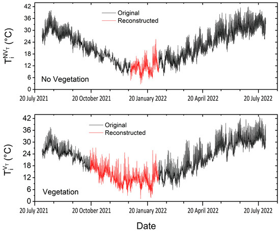
Figure 4.
The whole calendar year dataset as originally measured (black line) for the non-vegetated wall (top panel) and the vegetated wall (bottom panel) and as reconstructed after comparison with the closest ARPA weather station (red line).
Figure 4.
The whole calendar year dataset as originally measured (black line) for the non-vegetated wall (top panel) and the vegetated wall (bottom panel) and as reconstructed after comparison with the closest ARPA weather station (red line).
The uncertainty associated with the T-reconstructed time series (ΔHRF) is, in total, ±0.5 °C (i.e., the sum of the three uncertainty values provided by assessing the accuracy of the BlueSky equipment, the ARPA thermometer, and the error propagation rounded to the first decimal).
4.1.2. Seasonal and Monthly Results
Table 2 reports the seasonal values of the measured temperature differences (NV wall minus V wall, i.e., data from the top–bottom panels in Figure 4). Negative values in Table 2 represent a warming effect caused by the VGS, while positive values represent a cooling effect. Overall, the VGS’s mean effect is a cooling effect, as 0.3 < .
Table 2.
Seasonal temperature differences between NV and V walls (min, max, and mean) during the day, during the night, on NRDs, and on RDs over the monitored period.
Table 2.
Seasonal temperature differences between NV and V walls (min, max, and mean) during the day, during the night, on NRDs, and on RDs over the monitored period.
| Season | (TNV-TV)day (°C) | (TNV-TV)night (°C) | (TNV-TV)RD (°C) | (TNV-TV)NRD (°C) | ||||||||
|---|---|---|---|---|---|---|---|---|---|---|---|---|
| Min | Max | Mean | Min | Max | Mean | Min | Max | Mean | Min | Max | Mean | |
| Summer | −6.8 | 7.4 | 2.1 | −6.8 | 5.8 | 1.1 | −2.6 | 6.1 | 1.6 | −6.8 | 7.4 | 2.1 |
| Autumn | −7.2 | 8.7 | 2.8 | −2.4 | 7.6 | 2.2 | −2.9 | 8.7 | 1.9 | −7.2 | 7.9 | 2.9 |
| Winter | −10.3 | 7.7 | 0.8 | −4.8 | 7.7 | 0.8 | −6.7 | 7.0 | 1.2 | −10.3 | 7.7 | 0.8 |
| Spring | −8.7 | 8.1 | 0.8 | −5.9 | 4.9 | 0.5 | −2.1 | 2.3 | 0.3 | −8.7 | 8.1 | 0.9 |
Note: The day is considered to last from 8:00 to 19:00 and the night is considered to last from 20:00 to 7:00.
In autumn, the mean cooling values are the highest among all of the seasons. During the day, the bare wall is, according to the mean, 2.8 °C warmer than the vegetated wall, while at nighttime this difference is 2.2 °C. The diurnal effect of the VGS in fall ranges from a warming influence (−7.2 °C) to a cooling influence (8.7 °C). Similarly, in the night, such effect is slightly reduced, with the warming influence being much less visible (−2.4 °C) and the cooling effect still being effective (7.6 °C). It is especially during the rainy days that a decrease in the warming capability of the VGS is observed.
Summer shows a similar warming effect in the day and night (albeit reduced on cloudy days): while the VGS shows an average diurnal cooling effect of 2.1 °C at the maximum peaks, the cooling effect reaches 7.4 °C during the NRDs.
In winter, during the daytime and especially on NRDs, the VGS shows that despite the maximum warming capacity fluctuating over the season, the overall effect is still, on average, a cooling effect of 0.8 °C. The VGS’s warming effect mainly reduces during the night and on rainy days. In late winter and early spring, the VGS does not show any bias in directing cooling/warming effects: it shows values fluctuating almost symmetrically, with the maximum symmetrical variability in warming and cooling effects occurring during the daytime on NRDs (about ±8.4 °C) and the minimum occurring on rainy days (about ±2.2 °C).
These findings coincide with the phenological growing patterns of the vegetation. When the mass of vegetation or leaves reaches its maximum (i.e., in summer and autumn), the thermal impact is the highest. However, during the dormant period (i.e., winter) and early stage of the growing period (i.e., spring), this impact is lower. The consistent mean values above 0 °C indicate that the VGS consistently maintained cooler temperatures compared to the bare wall during the analysed calendar year, offering valuable insights into the role of vegetation in influencing microclimates and, above all, in reducing global warming’s effects during these seasons. The results described in Figure 5 and Figure 6 highlight how the vegetation contributed to dynamically reducing the temperature in proximity to the wall surface, behaving similarly to an insulation layer. Such contribution is, however, not constant during the calendar year, and is rather more or less effective depending on the microclimatic conditions. The two TAnomaly,VGS representative thresholds that were identified through the data analysis explained in Section 3.2 overlapped with the vegetation’s growing season (GS). The first TAnomaly,VGS threshold can be extracted looking at the minimum T value during the GS, i.e., TAnomaly,VGS = 2.6 °C, as is visible in Figure 6 (optimal conditions, green areas in Figure 5 and Figure 6), while the second TAnomaly,VGS threshold refers to the risk of frost damage and/or low greenery growth, which may occur when there is a concomitant effect of rainfall/snowfall presence with temperatures lower than zero and/or cold-spell climate events (red areas in Figure 5). In such conditions, the vegetation limits its cooling potential, i.e., the decrease in temperature is limited. The results described in Figure 5 show that the periods with optimal conditions occur most frequently in the summer months after significant rainfall. The inter-week durability of optimal conditions can, however, last up to mid-October (Figure 5a, green areas). The red areas during the winter months highlight the period in which the risk of the vegetation being damaged due to freezing is high, while the red areas during spring highlight climatic cold spells or chilly nights.
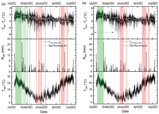
Figure 5.
(a) One-year monitored data (top panel) for the temperature differences of the NV and V walls with inter-weekly running averages, and the precipitation (central panel) and temperature (bottom panel) from the ARPA (AR subscript) weather station in Milan; (b) (from top to bottom) 1-year data for the temperature differences of the NV and V walls with weekly running averages, and the precipitation, and temperature in Milan. Green areas refer to optimal conditions, while red areas represent the risk of frost damage and/or low greenery growth due to cold-spell climate events. As introduced above, the monthly variability of the NV and V mean temperatures (Figure 6b, thick black and green lines, respectively) and TAnomaly,VGS are described in Figure 6 together with the optimal GS. The zero value of TAnomaly,VGS in April–May (see the coincident peaks of the black and green lines in Figure 6b) coincides with the beginning of the vegetation growth (i.e., the GS’s start time). The maximum impact of the vegetation occurs in the months from July to October, when the foliage is more luxuriant, contributing to an efficient cooling effect. Both Figure 5 and Figure 6 clearly show the identification of a period of stress on the vegetation and the optimal GS, and this phenological growing pattern is aligned with the thermal cooling impact.
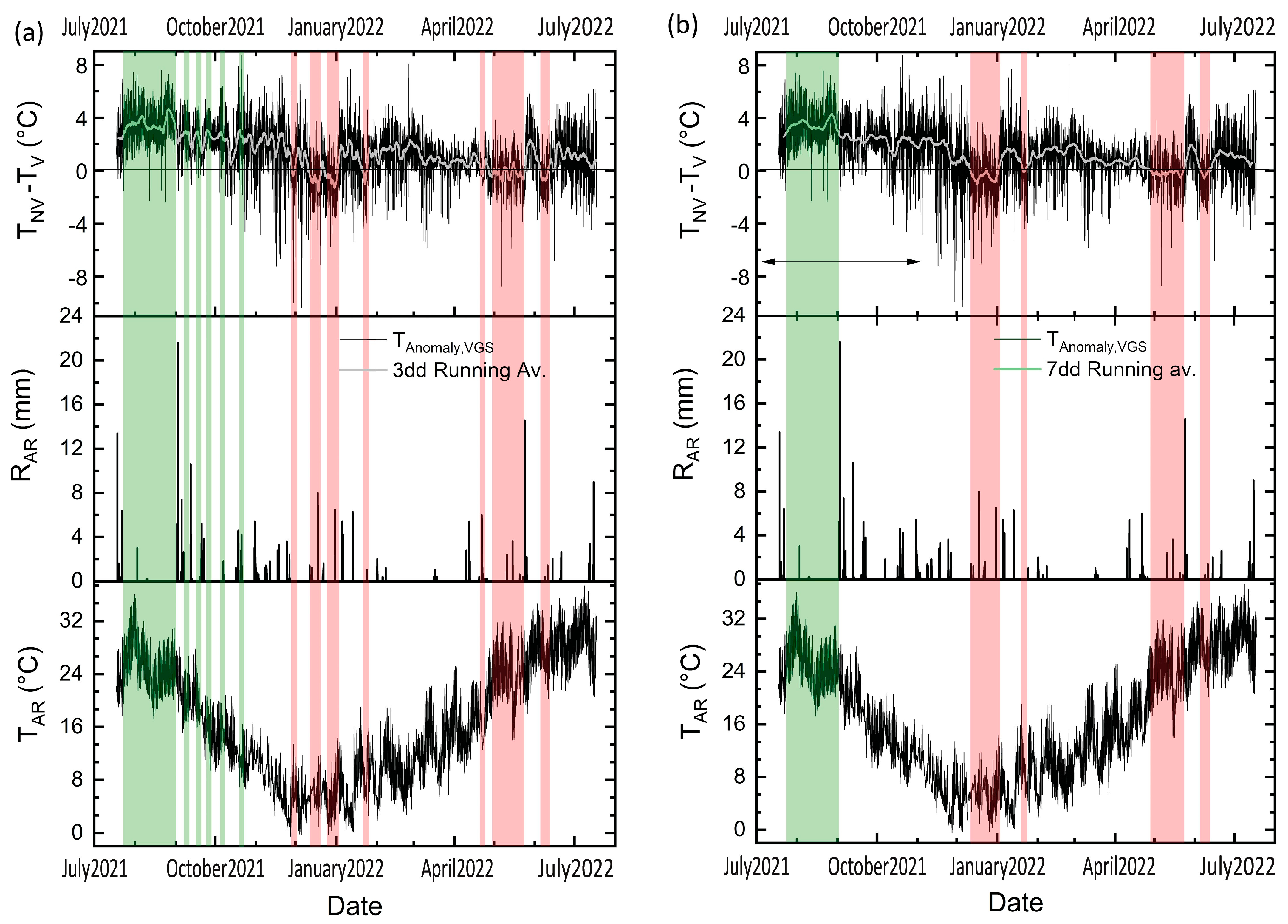
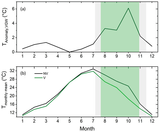
Figure 6.
(a) Monthly anomalies and (b) monthly mean temperatures of the NV and V walls over the monitored calendar year. The green area highlights the GS period.
Figure 6.
(a) Monthly anomalies and (b) monthly mean temperatures of the NV and V walls over the monitored calendar year. The green area highlights the GS period.
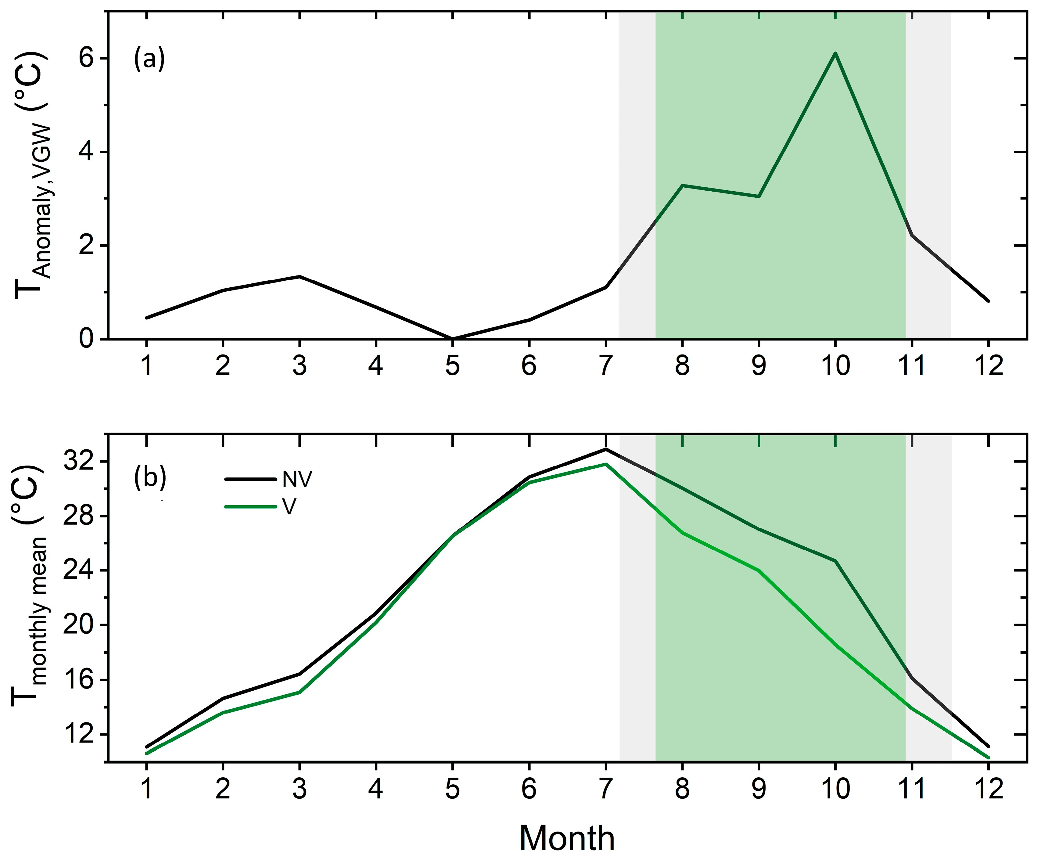
Figure 7a reports both the anomalies in the climatic conditions recorded over the monitored period of 2021–2022 with respect to the typical annual climate over the NP period (1991–2020), and the cooling/warming effect of the V wall with respect to the NV wall. The plot clearly highlights the GS starting month (i.e., coincident orange and green dots in May), as well as the overall cooling effect of the V wall that—in each month—shows a zT value lower than that of its NV counterpart. In the plot, the months with the larger cooling effects are those within the GS (i.e., July, August, September, and October). Taking into consideration the total error of ±0.8 °C constituted by the accuracy of the instruments (i.e., the BlueSky and ARPA T sensors, in total equalling ±0.3 °C), that of the ΔZ = ±0.45 °C. The seasons that can be considered anomalous over the 2021–2022 period, with respect to the typical T and precipitation conditions over the NP period, are the spring and summer of 2022, being generally warmer and drier (with autumn 2021 being similar to the NP period). In May (month 5), both the rain and T indices of the NV and V walls overlap, and therefore this month can be selected as the GS starting point and as the zero level for the TAnomaly,VGS in Figure 7b. This figure shows the impact of frequent hot spells on the state of vegetation, relating TAnomaly,VGS with the difference in the number of heatwave events with respect to the NP period (ΔNT>25 °C) for the months with vegetative activity (i.e., May–September) only. In detail, the x-axis shows the daily average of the NV–V temperature difference (i.e., TAnomaly,VGS), while the y-axis reports the difference in the number of times in the hourly data that T exceeds the threshold of T = 25 °C over the monitoring period (i.e., 2021–2022) with respect to the previous 7 days of the typical year in the NP period. The insulating power of the VGS is directly proportional to the luxuriance of the plants. The frequency of hot spells can have an impact on the health of the foliage, which may consequently—if subjected to frequent thermal stress—lower the value of TAnomaly,VGS. The relation of the VGS’s well-being is highlighted with the linear regression equation below:
The results described in Figure 7a,b show the further enhancement of climate anomalies and cooling/warming effects of the vegetation. Thanks to the newly developed rain and T indices, it was possible to quantify the degree of anomaly in the monitored period with respect to the reference years (visible in Figure 7a). Figure 7b in particular identifies vegetation stress states in relation to the frequency of hot spells and their effects in terms of reducing the cooling capability.

Figure 7.
(a) Rain and temperature indices for the NV (orange dots) and V (green dots) walls each month during the monitored period. (b) TAnomaly,VGS versus the difference in the number of heatwave events with respect to the NP period (ΔNT>25 °C) for the months with vegetative activity (i.e., May–September).
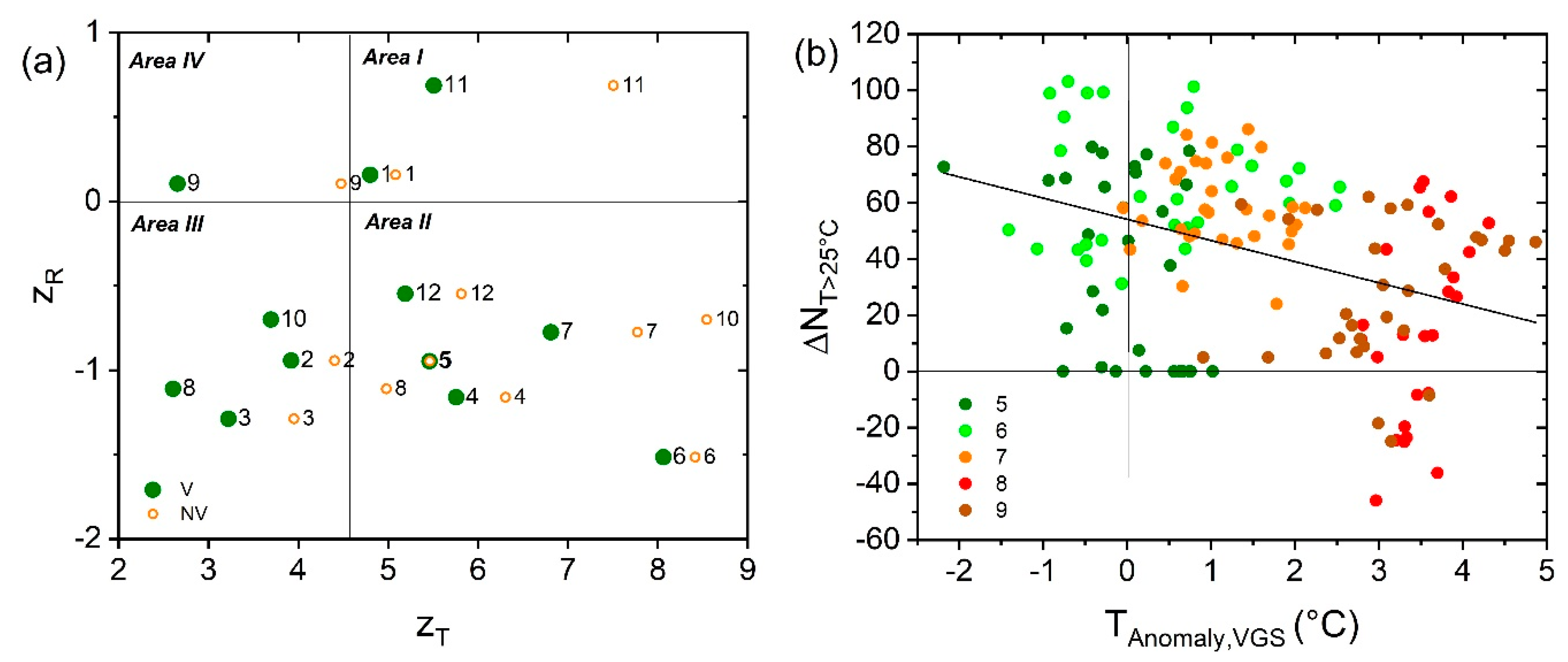

Figure 8.
Global warming (CC) effects, with reference to an EFP period, for the bare wall (white bars) and the vegetated wall (green bars). Grey area reports the error band.
Figure 8.
Global warming (CC) effects, with reference to an EFP period, for the bare wall (white bars) and the vegetated wall (green bars). Grey area reports the error band.
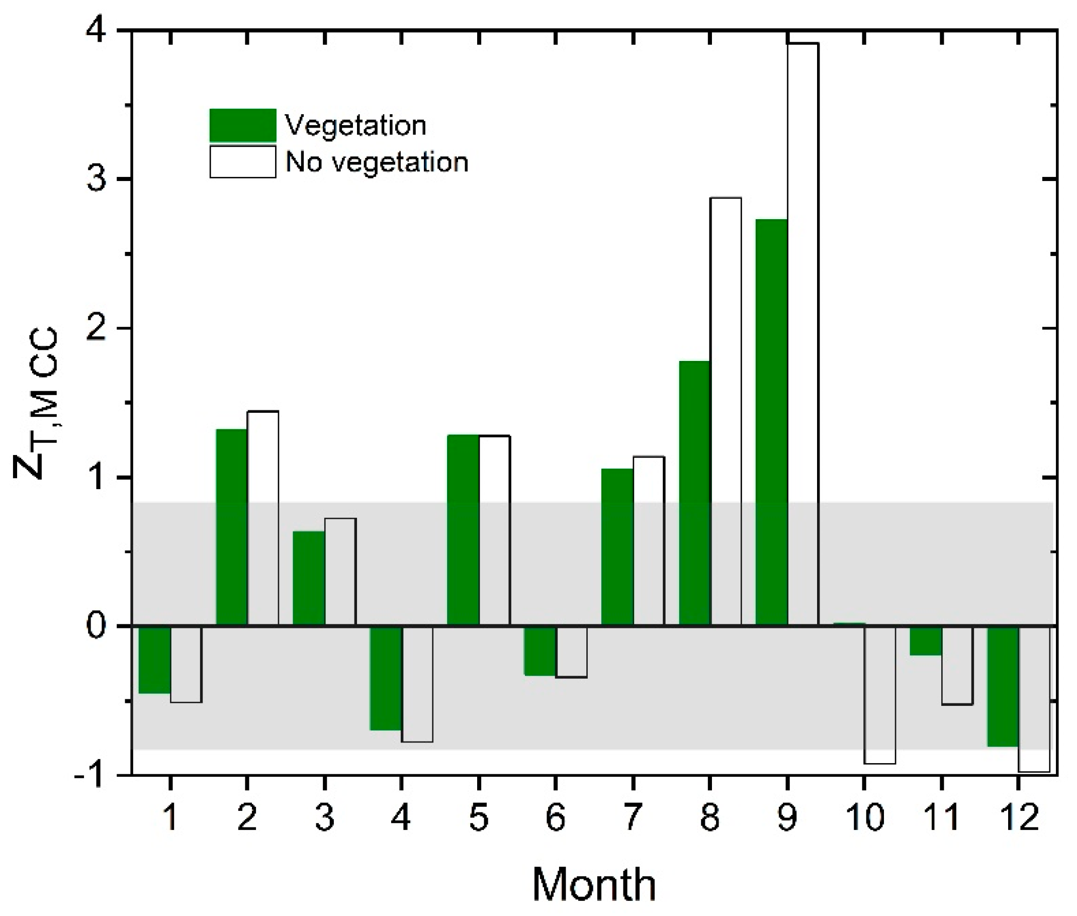
Finally, the last result obtained in this study is related to the VGS’s capacity to mitigate the local climate change (CC) impact using Equation (12) reported above. The index (i.e., zT,M CC) used to investigate the local CC mitigation achieved with the LW allows us to represent visually the T differences between the monitoring period and the extremely far-past (EFP) historical reference. When the index is above 0, it means that the contemporary monitored temperature in a specific month is higher than the temperature recorded in the corresponding month in the EFP, which is the expected case at present because of the concomitant effects of global warming and the existing urban core in the city centre. In contrast, values below 0 indicate that the monitored temperature nowadays is lower than the EFP reference average (for the corresponding month). However, the climate change indications need to be considered within the error band; once this is considered, the instrumental error and the propagation error exist in the range of ±0.8 °C, as highlighted by the grey band in Figure 8. In the plot, the warming effect in the proximity of the bare wall is represented by the white bars, while the same effect measured with the air T sensor embedded in the vegetation is denoted with the green bars. The effect of global warming is evident and intense with respect to the EFP in February and May, and from July to September. The GS months are also the ones when the most significant cooling impact driven by the VGS may be observed (lower green bars with respect to the white bars). This specific zT,M CC index helped us to estimate the impact of the global warming that occurred over a period of circa 260 years in the city centre of Milan in an area spatially ranging between The Westin Palace and Brera Astronomical Observatory (1.3 km distance), and to observe the potential a VGW may have in reducing such warming (difference between the white and green bars in Figure 8).
4.2. Qualitative Comparison with the Existing Literature
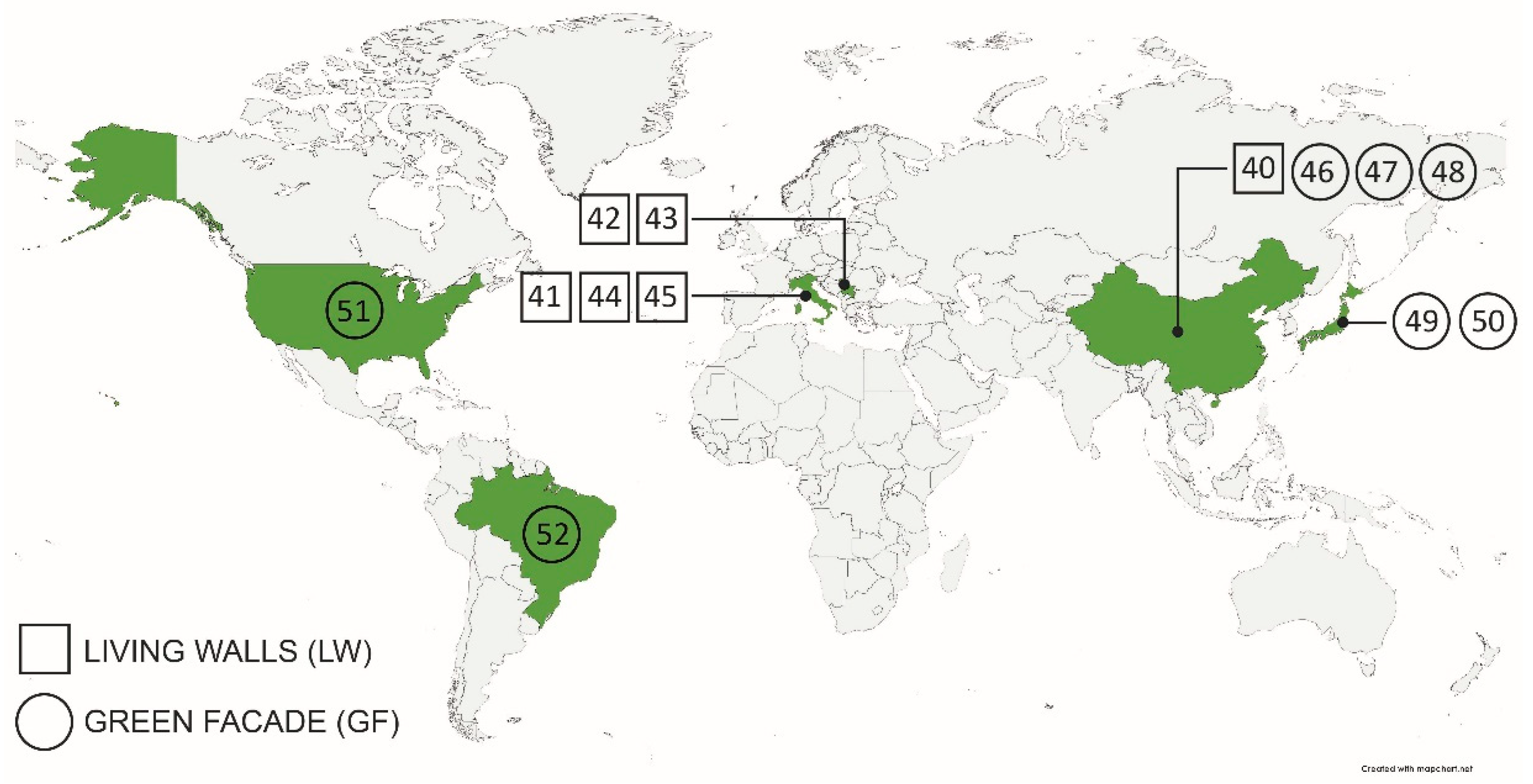
To compare the results achieved during the monitoring campaign and reported in Table 2 with those in the existing literature, a summary of the selected (as explained in Section 3.4) thirteen reviewed papers is reported in Table 3 below, while the locations of the VGS case studies reported in these papers are mapped in Figure 9. In the following, only the case studies reporting LWs in areas with the Cfa KG climate classification have been qualitatively compared with the same VGS typology installed in Milan (shown in bold in Table 3). Although, among the 13 selected papers, no LW case studies were found that faced the northwest direction (such as the LW on the hotel in Milan); however, the cases studies [32,33] were considered more representative in defining similarities with the present study. In [33], Serra et al. monitored an LW case, located in Turin (Italy), facing towards north during summer. They reported a maximum for the specie Lonicera nitida L. equal to 6.5 °C (7.4 ± 0.5 °C in our study during the 2021–2022 period; see Table 2). In the same season, Sudimac et al. [34,35] monitored an LW with Geranium macrorrhiuum, Cordifolia stock, and Nitida lemon facing south and located in Belgrade, Serbia. They found a maximum diurnal equal to 6.3 °C (7.4 ± 0.5 °C in our contribution); then, in detail, they found the mean during the day to be 1.7 °C for Geranium macrorrhiuum, 2.9 °C for Cordifolia stock, and 3.3 °C for Nitida lemon (2.1 ± 0.5 °C in our contribution). The authors concluded that the preferred species for inducing a cooling effect was Nitida lemon. In the paper in [32], the outcomes achieved with LWs facing W (located in Wuhan, China), monitored during summer and autumn periods, show a maximum range of surface temperature variability equal to 20.8 °C [32] (in our contribution, the maximum range of diurnal air T variation in summer and autumn is circa 15.0 ± 0.5 °C, as shown in Table 2). In addition to , Chen et al. measured the air temperature in the gap between a building façade and an LW, reporting a 9.7 °C T anomaly during the day and a 1.6 °C T anomaly during the night. According to these authors, a sealed air layer in the air gap performs better in its cooling ability than a naturally ventilated air layer. Moreover, a smaller air gap distance between the façade of the building and the green wall performs better as well. In [36], the authors studied two LWs facing SW, cultivated with several shrubs, grasses, and climber-plant species, located in Lonigo and Venice, northeastern Italy. During the monitored period (summer–autumn) in Lonigo, the had a total variability during NRDs of 20.0 °C, while in Venice, the total variability during NRDs was 16.0 °C (14.7 ± 0.5 °C in our contribution as an average between summer and autumn). The authors in [36] concluded that, because of the LW, the prevalence of outgoing heat fluxes had a significant advantage during the summer season as the presence of LW contributed to reducing the cooling load supplied by the HVAC system with a consequent reduction in the primary cooling energy consumption. On the other hand, only one study was conducted during the winter season, i.e., on an LW facing south located in Turin having a single species (Lonicera nitida L.). In this work, the maximum during NRDs was 8.0 °C [37] (in our contribution, this was 7.7 ± 0.5 °C). The authors in [37] also tested a second species, Bergenia cordifolia L. (not directly in the LW), obtaining interesting findings related to the visual damages observed on this species in microclimatic conditions with air temperatures < 10 °C. In these conditions, the Bergenia cordifolia L. showed damages in the form of frozen leaves that appeared burnt. This risk threshold can be related to our method of selecting risky periods, as highlighted in Figure 5.
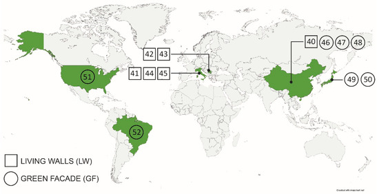
Figure 9.
Map of case studies from the 13 selected papers in the literature, coloured in green.
Figure 9.
Map of case studies from the 13 selected papers in the literature, coloured in green.
To sum up the qualitative comparison explained above, the results from Turin, Italy [37] (facing S, monitored in W) are aligned with the results presented in this contribution. In addition, similar cooling effects were observed with the species Geranium macrorrhiuum, as reported in [35], suggesting consistency with this contribution since this plant is also one of the cultivated plants in the LW in Milan, and it is close to the installed BluSky device. Our study tended to overestimate cooling effects compared to studies in other locations like Turin (Italy) [33] (facing N, monitored in S) and Belgrade (Serbia) [34,35] (facing S, monitored in S). On the contrary, studies such as [32] from Wuhan (China) and [36] from Lonigo and Venice observed more impactful cooling effects. These underestimations and overestimations could be due to several reasons, e.g., the unique microclimatic conditions in the specific areas in the city based on the morphology, the building geometry, in addition to the orientation, and the vegetation types. Regarding the vegetation types, even if the phenological attributes reported in Table 2 and Table 3 seem similar, the results vary as expected due the different orientations. The accuracy of the sensors and the duration of the data collection periods are other possible reasons for discrepancy, since other studies monitored for shorter periods with different sensors.
Table 3.
Report of results from the literature (KG climate class: Cfa). Bold text indicates parameters closely resembling the case study, used for qualitative comparison.
Table 3.
Report of results from the literature (KG climate class: Cfa). Bold text indicates parameters closely resembling the case study, used for qualitative comparison.
| Period | Reference | Orientation | Typology | Plants | Parameters |
|---|---|---|---|---|---|
| S | [33] | N | LW | W, E | (1) |
| [38] | S | GF | W, D, E′, T | (1) (2) (3) | |
| [34,35] | S | LW | H, D, E, T | (1) (2) (3) | |
| [39] | E | GF | W, D, E′, T | (1) (3) | |
| [40] | S, N | GF | H, E, T | (1) (2) (3) | |
| [41] | W, SW | GF | W, D, E′, T | (1) | |
| [42] | S | GF | H, W, D, E′, T | (1) | |
| S–A | [36] | SW | LW | H, D, T > W, E | (1) (2) (3) |
| [32] | W | LW | NS (6 species) | (1) | |
| [43] | S, W | GF | H < E < W, D, T | (1) (3) (4) | |
| W | [37] | S | LW | W, E | (2) (3) (4) |
| ALL | [44] | W | GF | W, D, T | (1) |
Notes: Period: Monitoring periods are represented by the first letters (e.g., S = summer). Orientation: The capital letters for orientation stand for the acronyms of cardinal directions (e.g., S = south). Plants: H = herbaceous, W = woody, D = deciduous, E = evergreen, E’ = semi-evergreen, T = tender. Parameters: (1) = (NVT-VT)day, (2) = (NVT-VT)night, (3) = (NVT-VT)sunny, (4) = (NVT-VT)cloudy (°C).
4.3. Future Climate Change Scenarios and Consequences for VGSs
As already stated, the KG climate classification of Milan is nowadays defined as Cfa. The KG classification was developed in the late 19th century [45], and its ranking still depends on the month-by-month threshold values and seasonality of air T and precipitation. Regions having the same KG climate class share common phenological attributes, as the climate has long since been recognised as the major driver of global vegetation distribution. Different areas worldwide can be compared using the KG climate classification for studying similarities or differences in climatic regimes, for vegetation and ecological modelling, or for assessing the impact of climate change. Therefore, the KG classification has a high potential to be used to forecast how variations in T and precipitation caused by climate change will influence (1) modifications in the selection of optimal vegetation species to be cultivated in a VGS to optimise its performance (e.g., to optimise the cooling effects provided by the vegetation); (2) the healthy state of the vegetation in the long run; (3) the VGS’s visual impact and durability, and the cost of its maintenance.
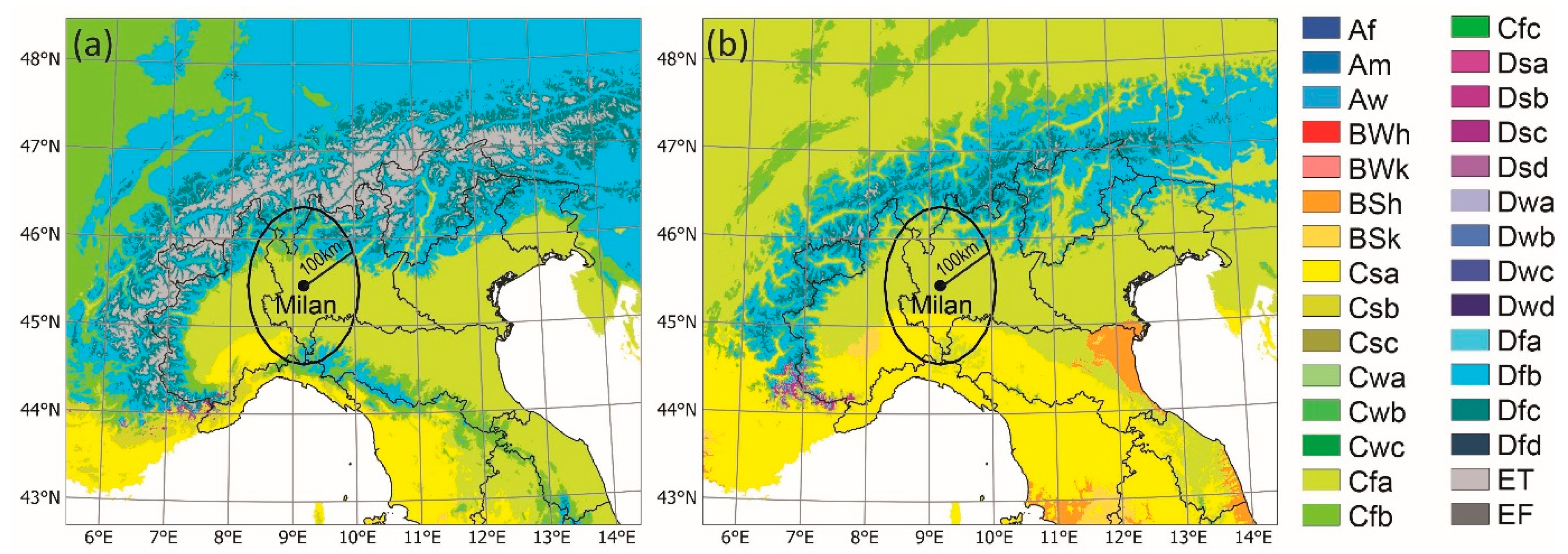
Notwithstanding, when dealing with KG climate classification, vegetation is usually considered as “crystallized in the visible (present) climate”, as stated in [46]; however, as clearly described by Beck et al. in 2018 [31], due to the ongoing climate change, it is expected that in few years from now, a same location will belong to a different KG climate class. In fact, fifty years from now, the impact of climate change will be clearly visible in terms of shifts in KG climate classes, or in their spatial enlargement or reduction, or in the modification of elevation gradients. Such shifts can be reconstructed into a future map (far-future period: 2071–2100, Figure 10b) to be compared towards a map close to the present (close-to-present period: 1980–2016, Figure 10a) using the database made available in [31]. The reconstruction of maps of the KG climate classification at a 1 km resolution is explained in detail in [31]. The present map is derived from an ensemble of four high-resolution, topographically corrected climatic maps, while the far-future map is derived from an ensemble of 32 climate model projections under the most severe scenario RCP8.5. Although Figure 10 shows that Milan will be not directly affected by a KG classification shift, its surrounding area (the area circled in the maps within a radius of 100 km), on the other hand, will be affected. In detail, in the far future, north of Milan, there will be a disappearance of the Cfb climate class (i.e., temperate climate without dry seasons and with warm summers) in the Lombard pre-Alps (i.e., the “Brianza” area), and a retreat of the Dfb KG climate class (i.e., cold climate without dry seasons and with warm summers) in all of the central Alps, departing from the Cfa temperate climate without dry seasons and with hot summers. Then, south of Milan, there will be the simultaneous disappearance of the Cfb and Dfb KG climate classes in the Ligurian Apennines and Tuscan-Emilian Apennines, and the progress of a Csa climate in the Po plain (i.e., a temperate climate with dry and hot summers). These forecasts highlight important insights for the future of building designs and urban planning that aims for the healthy lives of citizens, emphasising the importance of LWs among the sustainable strategies for regulating microclimates affected by global warming, especially in urban areas.
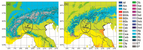
Figure 10.
Present and future Köppen–Geiger classifications of the Alps, northern Italy, and central Italy: (a) shows the map close to the present (1980–2016), and (b) shows the far-future map (2071–2100) (produced after [31]).
Figure 10.
Present and future Köppen–Geiger classifications of the Alps, northern Italy, and central Italy: (a) shows the map close to the present (1980–2016), and (b) shows the far-future map (2071–2100) (produced after [31]).
5. Conclusions and Further Research
In conclusion, this contribution presents a comprehensive analysis of the microclimate surrounding an LW in Milan by focusing on in situ temperature measurements recorded on a bare wall and a vegetated wall during one year. This monitoring duration adds value to this study with respect to the existing literature, as all of the seasons are covered, while most existing studies report short-term monitoring campaigns. Moreover, our data analysis aimed to assess the VGS’s capability for thermal regulation, as well as for the mitigation of urban heat in an urban area. In the monitoring period, some technical issues resulted in data gaps; however, thanks to the existing ARPA databases, this gap was filled with a novel reconstruction method.
Based on our dataset analysis, we found significant insights into the potential of VGSs in regulating microclimates and mitigating the adverse effects of high temperatures, especially during summer and autumn, when vegetation growth is at its peak. The LW consistently maintained cooler temperatures compared to the NV wall, particularly when growing conditions were optimal, such as during precipitation events. We identified threshold values for optimal growth and frost risk, indicating periods when cooling effects may be compromised. During summer, the vegetation helped to lower the wall temperatures, countering the warming effects common in urban areas due to CC and the UHI effect. However, in winter or spring, frost damage from cold spells threatened the vegetation’s survival, reducing its cooling effectiveness.
A historical dataset (EFP) was utilised to estimate the VGS’s potential for mitigating CC. A comparison with the EFP dataset revealed that in Milan, CC events over the past 260 years have been most notable in February, May, and from July to September, highlighting the significant contribution of VGSs to temperature reduction during these months. These findings underscore the importance of VGSs in mitigating the effects of CC and providing sustainable design solutions to enhance environmental conditions in densely built areas. Installing VGSs in compact urban environments offers promising benefits for climate change mitigation and adaptation, as well as sustainable urban development. This solution is particularly crucial given the projected shifts in global climate classifications (KG) expected within the next 50 years. Strategically installing vegetation types capable of withstanding these new climate projections on building envelopes can play a pivotal role in mitigating the global warming effect, offering an effective passive solution.
Lastly, a qualitative comparison between the seasonal data monitored in this study (Table 2) and those extracted from the literature (Table 3) offered insights into the thermal regulation capabilities of VGSs. Despite the promising findings, the performance of VGSs in building envelopes depends on various parameters beyond temperature anomalies, e.g., the local climate, the aspect direction, and the VGS’s typology, individual components, and cultivated species. Since identical studies were not available in the literature, the most similar case studies were selected for qualitative comparison. The comparison revealed that the highest observed mean temperature differences were detected in autumn, followed by summer, highlighting the cooling effect during these seasons, albeit with varying degrees of impact. Additionally, threshold values for optimal growing conditions and the risk of frost among the vegetation were similarly identified in the literature.
The limitations of this study are mainly related to the small number of sensors used for sampling the VGS, which was requested by the building owner in order to limit the visual impact of the monitoring devices; the assumption that the air temperature data measured with the sensors in contact with the non-vegetated and vegetated areas were in thermal equilibrium with their respective surfaces; and, finally, the error introduced in the period of the temperature time series that was reconstructed in order to fill the gaps in the data that occurred during the monitoring campaign.
Author Contributions
O.O.: Conceptualisation, writing—original draft preparation, data curation, formal analysis, visualisation. J.N.T.: Conceptualisation, writing—review and editing, supervision, funding acquisition as a Ph.D. supervisor and through the HARMONIA H2020 project. S.C.: Data reconstruction and curation, formal analysis, writing—original draft preparation. C.B.: Conceptualisation, formal analysis, writing—original draft preparation, writing—review and editing, supervision, funding acquisition as a Ph.D. supervisor. All authors have read and agreed to the published version of the manuscript.
Funding
This paper is funded by the HARMONIA project under grant number 101003517 since the corresponding author is the coordinator of the HARMONIA project. Furthermore, this work was possible within the framework of the PhD scholarship in co-supervision with Politecnico di Milano (POLIMI) and the Norwegian University of Science and Technology (NTNU) under the cotutelle PhD agreement of the first author.
Data Availability Statement
The raw data supporting the conclusions of this article will be made available by the authors on request.
Acknowledgments
The authors would like to acknowledge Maria Vittoria Beatrici, and Gianluca Carrao from the electricity section of The Westin Palace for all of their support and collaboration during this monitoring campaign.
Conflicts of Interest
The authors have no competing interests to declare.
Abbreviations
| ARPA | Regional Agency for Protection and the Environment |
| Cfa | temperate climate without dry seasons and with hot summers (T ≥ 22) |
| EFP | extremely far past (1763–1792) |
| NP | near past (1991–2020) |
| GF | green façade |
| GS | growing season |
| H | herbaceous |
| W | woody |
| D | deciduous |
| E | evergreen |
| E’ | semi-evergreen |
| T | tender |
| HISTALP | Historical Instrumental Climatological Surface Time Series of the Greater Alpine Region |
| KG | Köppen–Geiger |
| LW | living wall |
| N | north |
| W | west |
| S | south |
| E | east |
| NRD | no rainy days |
| NV | non-vegetated |
| NW | northwest |
| NE | northeast |
| SW | southwest |
| SE | southeast |
| NTC | Negative Temperature Coefficient |
| PM | particulate matter |
| RDs | rainy days |
| S | summer |
| A | autumn |
| W | winter |
| SP | spring |
| T | temperature |
| V | vegetated |
| VGS | vertical green structure |
References
- Alcoforado, M.J.; Andrade, H. Global Warming and the Urban Heat Island. In Urban Ecology: An International Perspective on the Interaction between Humans and Nature; Springer: Boston, MA, USA, 2008; pp. 249–262. ISBN 978-0-387-73412-5. [Google Scholar] [CrossRef]
- Shahmohamadi, P.; Che-Ani, A.I.; Maulud, K.N.A.; Tawil, N.M.; Abdullah, N.A.G. The Impact of Anthropogenic Heat on Formation of Urban Heat Island and Energy Consumption Balance. Urban Stud. Res. 2011, 2011, 497524. [Google Scholar] [CrossRef]
- Leal Filho, W.; Echevarria Icaza, L.; Neht, A.; Klavins, M.; Morgan, E.A. Coping with the Impacts of Urban Heat Islands. A Literature Based Study on Understanding Urban Heat Vulnerability and the Need for Resilience in Cities in a Global Climate Change Context. J. Clean Prod. 2018, 171, 1140–1149. [Google Scholar] [CrossRef]
- He, B.J.; Wang, W.; Sharifi, A.; Liu, X. Progress, Knowledge Gap and Future Directions of Urban Heat Mitigation and Adaptation Research through a Bibliometric Review of History and Evolution. Energy Build. 2023, 287, 112976. [Google Scholar] [CrossRef]
- Ogut, O.; Tzortzi, N.J.; Bertolin, C. Vertical Green Structures to Establish Sustainable Built Environment: A Systematic Market Review. Sustainability 2022, 14, 12349. [Google Scholar] [CrossRef]
- Zaid, S.M.; Perisamy, E.; Hussein, H.; Myeda, N.E.; Zainon, N. Vertical Greenery System in Urban Tropical Climate and Its Carbon Sequestration Potential: A Review. Ecol. Indic. 2018, 91, 57–70. [Google Scholar] [CrossRef]
- Charoenkit, S.; Yiemwattana, S. Role of Specific Plant Characteristics on Thermal and Carbon Sequestration Properties of Living Walls in Tropical Climate. Build. Environ. 2017, 115, 67–79. [Google Scholar] [CrossRef]
- Pandey, A.K.; Pandey, M.; Tripathi, B.D. Assessment of Air Pollution Tolerance Index of Some Plants to Develop Vertical Gardens near Street Canyons of a Polluted Tropical City. Ecotoxicol. Environ. Saf. 2016, 134, 358–364. [Google Scholar] [CrossRef] [PubMed]
- Jeong, N.R.; Kim, J.H.; Han, S.W.; Kim, J.C.; Kim, W.Y. Assessment of the Particulate Matter Reduction Potential of Climbing Plants on Green Walls for Air Quality Management. J. People Plants Environ. 2021, 24, 377–387. [Google Scholar] [CrossRef]
- Collins, R.; Schaafsma, M.; Hudson, M.D. The Value of Green Walls to Urban Biodiversity. Land Use Policy 2017, 64, 114–123. [Google Scholar] [CrossRef]
- Shafiee, E.; Faizi, M.; Yazdanfar, S.A.; Khanmohammadi, M.A. Assessment of the Effect of Living Wall Systems on the Improvement of the Urban Heat Island Phenomenon. Build. Environ. 2020, 181, 106923. [Google Scholar] [CrossRef]
- Price, A.; Jones, E.C.; Jefferson, F. Vertical Greenery Systems as a Strategy in Urban Heat Island Mitigation. Water Air Soil Pollut. 2015, 226, 247. [Google Scholar] [CrossRef]
- Maier, D. Perspective of Using Green Walls to Achieve Better Energy Efficiency Levels. A Bibliometric Review of the Literature. Energy Build. 2022, 264, 112070. [Google Scholar] [CrossRef]
- Bustami, R.A.; Belusko, M.; Ward, J.; Beecham, S. Vertical Greenery Systems: A Systematic Review of Research Trends. Build. Environ. 2018, 146, 226–237. [Google Scholar] [CrossRef]
- Eumorfopoulou, E.A.; Kontoleon, K.J. Experimental Approach to the Contribution of Plant-Covered Walls to the Thermal Behaviour of Building Envelopes. Build. Environ. 2009, 44, 1024–1038. [Google Scholar] [CrossRef]
- Carlucci, S.; Charalambous, M.; Tzortzi, J.N. Monitoring and Performance Evaluation of a Green Wall in a Semi-Arid Mediterranean Climate. J. Build. Eng. 2023, 77, 107421. [Google Scholar] [CrossRef]
- Cuce, E. Thermal Regulation Impact of Green Walls: An Experimental and Numerical Investigation. Appl. Energy 2017, 194, 247–254. [Google Scholar] [CrossRef]
- Perini, K.; Ottelé, M.; Fraaij, A.L.A.; Haas, E.M.; Raiteri, R. Vertical Greening Systems and the Effect on Air Flow and Temperature on the Building Envelope. Build. Environ. 2011, 46, 2287–2294. [Google Scholar] [CrossRef]
- Sternberg, T.; Viles, H.; Cathersides, A. Evaluating the Role of Ivy (Hedera Helix) in Moderating Wall Surface Microclimates and Contributing to the Bioprotection of Historic Buildings. Build. Environ. 2011, 46, 293–297. [Google Scholar] [CrossRef]
- Köhler, M. Green Facades-a View Back and Some Visions. Urban Ecosyst 2008, 11, 423–436. [Google Scholar] [CrossRef]
- Ottelé, M.; Perini, K. Comparative Experimental Approach to Investigate the Thermal Behaviour of Vertical Greened Façades of Buildings. Ecol. Eng. 2017, 108, 152–161. [Google Scholar] [CrossRef]
- Bacci, P.; Maugeri, M. The Urban Heat Island of Milan. Nuovo Cimento 1992, 15, 417–424. Available online: https://www.researchgate.net/publication/227088821_The_urban_heat_island_of_Milan (accessed on 19 July 2023). [CrossRef]
- Kottek, M.; Grieser, J.; Beck, C.; Rudolf, B.; Rubel, F. World Map of the Köppen-Geiger Climate Classification Updated. Meteorol. Z. 2006, 15, 259–263. [Google Scholar] [CrossRef] [PubMed]
- Peverelli Design, Construction and Maintenance of Green—Peverelli Garden Design, Construction and Maintenance of Green. Available online: https://www.peverelli.it/en/ (accessed on 25 November 2022).
- BlueSky Air Quality Monitor 8143|TSI. Available online: https://tsi.com/products/environmental-air-monitors/bluesky-air-quality-monitor/ (accessed on 25 November 2022).
- Form Richiesta Dati—ARPA Lombardia. Available online: https://www.arpalombardia.it/temi-ambientali/meteo-e-clima/form-richiesta-dati/ (accessed on 19 July 2023).
- HISTALP. Available online: https://zamg.ac.at/histalp/ (accessed on 19 July 2023).
- Auer, I.; Böhm, R.; Jurkovic, A.; Lipa, W.; Orlik, A.; Potzmann, R.; Schöner, W.; Ungersböck, M.; Matulla, C.; Briffa, K.; et al. HISTALP—Historical Instrumental Climatological Surface Time Series of the Greater Alpine Region. Int. J. Climatol. 2007, 27, 17–46. [Google Scholar] [CrossRef]
- Guide to Instruments and Methods of Observation Volume I-Measurement of Meteorological Variables. Available online: https://library.wmo.int/records/item/68695-guide-to-instruments-and-methods-of-observation?language_id=13&back=&offset= (accessed on 19 July 2023).
- Stagnaro, M.; Colli, M.; Giovanni Lanza, L.; Wai Chan, P. Performance of Post-Processing Algorithms for Rainfall Intensity Using Measurements from Tipping-Bucket Rain Gauges. Atmos. Meas. Tech. 2016, 9, 5699–5706. [Google Scholar] [CrossRef]
- Beck, H.E.; Zimmermann, N.E.; McVicar, T.R.; Vergopolan, N.; Berg, A.; Wood, E.F. Present and Future Köppen-Geiger Climate Classification Maps at 1-Km Resolution. Sci. Data 2018, 5, 180214. [Google Scholar] [CrossRef] [PubMed]
- Chen, Q.; Li, B.; Liu, X. An Experimental Evaluation of the Living Wall System in Hot and Humid Climate. Energy Build. 2013, 61, 298–307. [Google Scholar] [CrossRef]
- Serra, V.; Bianco, L.; Candelari, E.; Giordano, R.; Montacchini, E.; Tedesco, S.; Larcher, F.; Schiavi, A. A Novel Vertical Greenery Module System for Building Envelopes: The Results and Outcomes of a Multidisciplinary Research Project. Energy Build. 2017, 146, 333–352. [Google Scholar] [CrossRef]
- Sudimac, B.; Ilić, B.; Munćan, V.; Anđelković, A.S. Heat Flux Transmission Assessment of a Vegetation Wall Influence on the Building Envelope Thermal Conductivity in Belgrade Climate. J. Clean Prod. 2019, 223, 907–916. [Google Scholar] [CrossRef]
- Sudimac, B.S.; Ignjatovic, N.D.C.; Ignjatovic, D.M. Experimental Study on Reducing Temperature Using Modular System for Vegetation Walls Made of Perlite Concrete. Therm. Sci. 2018, 22, 1059–1069. [Google Scholar] [CrossRef]
- Mazzali, U.; Peron, F.; Romagnoni, P.; Pulselli, R.M.; Bastianoni, S. Experimental Investigation on the Energy Performance of Living Walls in a Temperate Climate. Build. Environ. 2013, 64, 57–66. [Google Scholar] [CrossRef]
- Bianco, L.; Serra, V.; Larcher, F.; Perino, M. Thermal Behaviour Assessment of a Novel Vertical Greenery Module System: First Results of a Long-Term Monitoring Campaign in an Outdoor Test Cell. Energy Effic. 2017, 10, 625–638. [Google Scholar] [CrossRef]
- Li, C.; Wei, J.; Li, C. Influence of Foliage Thickness on Thermal Performance of Green Façades in Hot and Humid Climate. Energy Build. 2019, 199, 72–87. [Google Scholar] [CrossRef]
- Yin, H.; Kong, F.; Middel, A.; Dronova, I.; Xu, H.; James, P. Cooling Effect of Direct Green Façades during Hot Summer Days: An Observational Study in Nanjing, China Using TIR and 3DPC Data. Build. Environ. 2017, 116, 195–206. [Google Scholar] [CrossRef]
- Yang, F.; Yuan, F.; Qian, F.; Zhuang, Z.; Yao, J. Summertime Thermal and Energy Performance of a Double-Skin Green Facade: A Case Study in Shanghai. Sustain. Cities Soc. 2018, 39, 43–51. [Google Scholar] [CrossRef]
- Hoyano, A. Climatological Uses of Plants for Solar Control and the Effects on the Thermal Environment of a Building. Energy Build. 1988, 11, 181–199. [Google Scholar] [CrossRef]
- Koyama, T.; Yoshinaga, M.; Hayashi, H.; Maeda, K.I.; Yamauchi, A. Identification of Key Plant Traits Contributing to the Cooling Effects of Green Façades Using Freestanding Walls. Build. Environ. 2013, 66, 96–103. [Google Scholar] [CrossRef]
- Price, J.W. Green Façade Energetics. Master’s Thesis, University of Maryland, College Park, Maryland, 2010. [Google Scholar]
- Fensterseifer, P.; Gabriel, E.; Tassi, R.; Piccilli, D.G.A.; Minetto, B. A Year-Assessment of the Suitability of a Green Façade to Improve Thermal Performance of an Affordable Housing. Ecol. Eng. 2022, 185, 106810. [Google Scholar] [CrossRef]
- Der Erde, W.K.D.W.; Der Dauer Der Heissen, N. Gemässigten Und Kalten Zeit Und Nach Der Wirkung Der Wärme Auf Die Organische Welt Betrachtet. Meteorol.Ztg. 1884, 1, 215–226. [Google Scholar]
- Köppen, W. Das Geographische System Der Klimate, Handbuch Der Klimatologie [The Geographical System of the Climate, Handbook of Climatology]; Gebrüder Borntraeger: Berlin, Germany, 1936. [Google Scholar]
Disclaimer/Publisher’s Note: The statements, opinions and data contained in all publications are solely those of the individual author(s) and contributor(s) and not of MDPI and/or the editor(s). MDPI and/or the editor(s) disclaim responsibility for any injury to people or property resulting from any ideas, methods, instructions or products referred to in the content. |
© 2024 by the authors. Licensee MDPI, Basel, Switzerland. This article is an open access article distributed under the terms and conditions of the Creative Commons Attribution (CC BY) license (https://creativecommons.org/licenses/by/4.0/).