Spatio-Temporal Dynamics Coupling between Land Use/Cover Change and Water Quality in Dongjiang Lake Watershed Using Satellite Remote Sensing

Abstract

With rapid social and economic development, land use/land cover change (LUCC) has intensified with serious impacts on water quality in the watershed. In this study, we took Dongjiang Lake watershed as the study area and obtained measured data on water quality parameters from the watershed’s water quality monitoring stations. Based on Landsat-5, Landsat-8, or Sentinel-2 remote sensing data for multiple periods per year between 1992 and 2022, the sensitive satellite bands or band combinations of each water quality parameter were determined. The Random Forest method was used to classify the land use types in the watershed into six categories, and the area proportion of each type was calculated. We established machine learning regression models and polynomial regression models with WQI as the dependent variable and the area proportion of each land use type as the independent variable. Accuracy test results showed that, among them, the quadratic cubic polynomial regression model with grassland, forest land, construction land, and unused land as its independent variables was the best model for coupling watershed water quality with LUCC. This study’s results provide a scientific basis for monitoring spatial and temporal changes in water quality caused by LUCC in the Dongjiang Lake watershed.

1. Introduction

Rapid changes in land use structure and spatial patterns significantly impact the sustainable socio-economic development of basins and the stability of regional ecosystems [1,2], posing a major concern for river water quality monitoring globally. The integration of land use and land cover change (LUCC) with water quality has become a standard approach in water resource management [3,4]. The relationship between land use and water quality is known to vary across spatial scales, ranging from stream buffers and riparian corridors to entire watersheds [5]. However, there is no consensus on how this relationship varies. Currently, domestic and international studies propose various methods for assessing water quality, including multivariate statistical methods [6,7], modeling [8], and the water quality identification index (WQI) method [9,10]. Among these, the WQI was originally designed by Horton [11] and has since been further developed [12]. The WQI consolidates multiple physical and chemical parameters into a single value, providing a comprehensive assessment of water quality while eliminating discrepancies that can arise from assessing individual parameters [13]. The conventional method of monitoring water quality through WQI relies on manual sampling and analysis. Şener et al. [10] used WQI to assess the water quality of the Aksu River in southwestern Turkey, and the results showed that the more effective water quality parameters were COD and magnesium (Mg). Mutair et al. [14] conducted a study on the temporal and spatial patterns of water quality in Kuwait Bay from 2009 to 2011 using cluster analysis based on WQI data. The study found that water quality is primarily affected by seasonal variations, coastal point source pollution, and discharges from the Shatt al-Arab. The manual sampling and analysis method can accurately obtain water quality data in multiple areas. However, it is expensive and limited by monitoring stations’ numbers and data completeness. In recent years, researchers have employed techniques like Geographic Information Systems (GIS) and satellite remote sensing to conduct rapid land use studies [15]. The application of these techniques to determine the relationship between land use and water quality has been a significant breakthrough for the in-depth analysis of the correlation between LUCC and WQI [10]. It is also crucial for decision making and optimal allocation for the sustainable use of regional soil and water resources [16]. Satellite remote sensing technology has rapidly developed, and its imagery has advantages, such as wide coverage, fast update speed, low data acquisition costs, and high stability [17]. As a result, it has become one of the most effective means of water quality analysis [17], widely used in long-term water quality monitoring. Najafzadeh et al. [18] proved the high effectiveness of estimating WQI using Landsat 8 OLI-TIRS images, taking the Hudson River as the study area. The use of LANDSAT 7 ETM+ satellite imagery to track the polluted waters of Medrano Creek as it flows into the Río de la Plata resulted in confirmation of the potential of using satellite imagery to track organic pollution in freshwater systems [19]. Also, Najafzadeh et al. [20] characterized the water quality of the Karun River using Landsat-7 ETM+ data.

Dongjiang Lake is an important watershed in China and a pilot area for water resources ecological compensation [21]. The basin is an important source of water resources in Hunan Province, providing a precious source of high-quality water for 13 counties/cities, including Changsha, Zhuzhou, Xiangtan, Hengyang, and Chenzhou [22], and the stability of water quality in the watershed is crucial for regional, social, and economic development.

Previous research on the correlation between land use and water quality has primarily focused on individual water quality parameters, neglecting comprehensive watershed evaluations. And remote sensing data can be influenced by mixed pixels, making inversion accuracy difficult to guarantee, suggesting the need for a more holistic approach to understanding these interactions. To address these issues, this paper selected the Dongjiang Lake Watershed as the study area. We investigated the impact of land use on water quality in the watershed using Landsat-5, Landsat-8, or Sentinel-2 satellite remote sensing data to reveal the coupling relationship between WQI and LUCC in the watershed at different spatial scales. The study results offer theoretical support for the comprehensive management of the Dongjiang Lake Watershed. We improved the parameters of various types of regression models to improve the adaptability of the models according to the needs of the study area [23] and the actual situation of the watershed [24,25]. The proposed method can effectively help to deeply understand the driving mechanisms behind water quality changes.

2. Materials and Methods

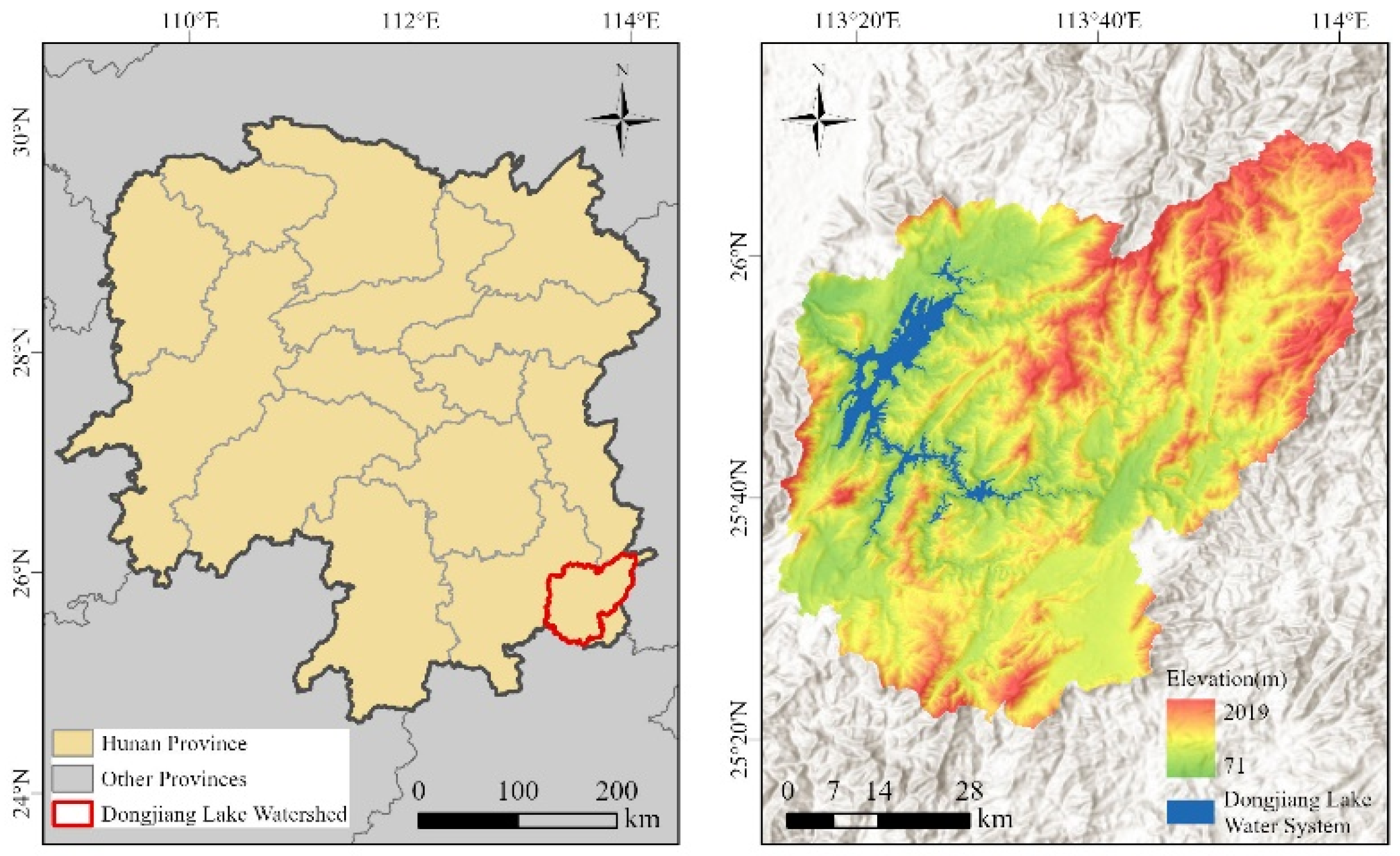
2.1. Study Area

Dongjiang Lake is situated in Zixing County-level City, Hunan Province (Figure 1), spanning a 113°08′–113°44′ east longitude and 25°34′–26°18′ north latitude. The watershed covers a total area of 4718 km², with a water surface area of 160 km², a total storage capacity of 974 million m³, and an average water depth of 61 m, making it one of the top ten freshwater lakes in China. The watershed originates from Yanzhubu Fort in Guidong County, and it covers four counties/cities, including Rucheng, Guidong, Zixing, and Yizhang, accounting for 43.31%, 27.62%, 26.04%, and 3.03% of the total watershed area, respectively (

Table 1. The area of the Dongjiang Lake Watershed in each administrative district and its proportion of the whole watershed.

County/City	Area in Each Administrative District (km2)	Area Proportion of the Whole Watershed (%)
Zixing County-Level City	1748.7	37.18
Rucheng County	1601.3	34.04
Guidong County	1234.7	26.25
Yizhang County	118.9	2.53
Total	4703.60	100

). The lake is fed by a total of 819 rivers, including Zheshui, Xianshui, Zixingjiang, Huojiang, and Hongjiang rivers. The upstreams of the secondary tributaries Zheshui, and Huojiang are located in the counties of Rucheng and Guidong, respectively. The soil types in the watershed are mainly red soil, yellow-red soil, yellow-brown soil, mountain meadow soil, and purple soil. The vegetation in the watershed belongs to subtropical evergreen broad-leaved forests, with a forest cover of 72%.

The Dongjiang Lake Watershed has 13 monitoring sections (

Table 2. Distribution of water quality monitoring stations in Dongjiang Lake Watershed.

Number	Water Body	Name of Water Quality Monitoring Section	Monitoring Frequency	Monitoring Affiliation
1	Dongjiang Lake	Xiaodongjiang Station	Once a month	Chenzhou City Station
2	Dongjiang Lake	Toushan Station	Once a month	Chenzhou City Station
3	Dongjiang Lake	Bailang Station	Once a month	Chenzhou City Station
4	Dongjiang Lake	Dongping	Once a quarter	Zixing City Station
5	Dongjiang Lake	Yanzipai Station	Once a quarter	Zixing City Station
6	Dongjiang Lake	Chukou Station	Once a quarter	Zixing City Station
7	Ou River	Chengguan Songshan Station	Once a month	Guidong County Station
8	Ou River	Chengguan Gaoqiao Station	Once a quarter	Guidong County Station
9	Ou River	Shibishan Hydropower Station	Once a quarter	Guidong County Station
10	Zheshui	Sigongqiao Station	Once a quarter	Rucheng County Station
11	Zheshui	Mantianxing Power Station	Once a quarter	Rucheng County Station
12	Zheshui	Longhudong Reservoir Station	Once a month	Rucheng County Station
13	Zheshui	Sandaianqiao Station	Once a quarter	Rucheng County Station

), including two monitoring sections in the primary protection area of the lake, namely, Xiaodongjiang and Toushan, and four in the secondary protection area of the lake, namely, Bailang, Chukou, Dongping, and Yanzipai. There are three in the Ou River section of the inlet rivers, including Chengguan Songshan Station, Chengguan Gaoqiao Station, and Shibishan Hydropower Station. Additionally, there are four in the Zheshui section of the inlet rivers, including Sigongqiao Station, Mantianxing Power Station, Sandaianqiao Station, and Longhudong Reservoir Station.

2.2. Data Resource

With the rapid development of satellite imaging technology, satellite remote sensing images have been widely used in monitoring the spatial and temporal dynamics of water resources due to their wide coverage, fast update speed, low data acquisition cost, and high stability. Commonly used data for water quality remote sensing monitoring are classified into high (<10 m), medium (10–200 m), and low (>200 m) spatial resolution, and appropriate spatial resolution data can be selected according to the size of the monitored waters. The low spatial resolution data are usually of low accuracy, but with short return periods, large monitoring areas, and simple data acquisition, making them suitable for monitoring large water bodies. Smaller catchments require high-precision data but such data have low temporal resolution, a long return period that limits continuous monitoring of the area, and high data acquisition costs that limit practical applications. Medium-resolution data have a moderate resolution that meets general monitoring requirements, a reasonable return period, and free access to the data, making medium-resolution data such as Landsat-5, Landsat-8, and Sentinel-2 the most widely used satellite remote sensing data for water quality monitoring.

2.3. Inversion of Water Quality Variables

Based on the water quality data of Dongjiang Lake obtained from the water quality monitoring stations in the watershed, this study identified the dissolved oxygen index (DO), permanganate index (COD_Mn), chemical oxygen demand index (COD), ammonia nitrogen index (NH₃-N) and total phosphorus index (TP) as the main water quality parameters in the study area [26]. The correlation relationship between each parameter and Landsat multispectral images was established, and the inversion models of five parameters were constructed. Among them, DO is an important indicator reflecting the self-purification ability of water bodies; the lower the DO, the more serious the degree of pollution in the water bodies [27]. The COD_Mn index refers to the amount of oxidant consumed by the unit of reducing substances in the water body that needs to be oxidized under specified conditions [28]; the higher the value of COD_Mn, the more the water bodies are polluted by organic and inorganic oxidizable substances [29]. COD refers to the amount of reducing substances in water samples that need to be oxidized and measured chemically, especially organic pollutants [30]; NH₃-N is a nutrient in the water body that can lead to the phenomenon of water eutrophication and is the main oxygen-consuming pollutant in the water body; TP is the total amount of phosphorus in the water body, and excess phosphorus can cause eutrophication of the water body and disturb the balance of the water body [31].

Table 3. Correlation coefficients between Landsat band combinations and measured data of DO, COD_Mn, COD, NH₃-N, and TP.

Band Combination	Band Combination Form	DO	CODMn	COD	NH3-N	TP
S1	b2 + b3	−0.19 *	0.21 **	0.33 **	−0.16 *	0.22 *
S2	b2 + b3 + b4	−0.18 *	0.22 **	0.33 **	−0.16 *	0.22 *
S3	b4/b2	0.04	0.18 *	0.25 *	−0.11 *	0.21 *
S4	b4/b3	−0.04	0.20 *	0.29 *	−0.11 *	0.23 *
S5	(b5 − b4) × (b5/b3)	0.87 **	−0.07	−0.13	−0.18 *	0.14
S6	(b3 + b4)/b2	0.08	0.12 *	0.18	−0.10	0.19
S7	b3/b2	0.08	0.24 **	0.29 *	−0.09	0.21 *
S8	b5/b3	0.60 **	0.25 **	0.32 **	−0.09	0.21 *
S9	(b3 + b5)/b2	0.12 *	0.19 *	0.24 *	−0.09	0.21 *
S10	(b2 + b5)/b3	−0.02	0.29 **	0.16	0.01	0.08
S11	b4 + b5	0.01	0.01	−0.04	0.06	0.01
S12	(b4 + b5)/(b2 − b3)	0.14 *	−0.04	−0.02	0.10	0.17
S13	b4/b5	−0.03	−0.24	−0.25 *	0.06	−0.18
S14	b2 + b3 + b5	−0.17 *	0.23 **	0.34 **	−0.16 *	0.23 *
S15	b2 + b3 + b4 + b5	−0.11	0.20 *	0.40 **	−0.16 *	0.30 **
S16	b6 − b7	0.15 *	0	0.04	0.03	0.05
S17	b2 + b3 + b6 + b7	−0.17 *	0.22 **	0.35 **	−0.16 *	0.23 *
S18	(b2 − b3)/(b2 + b3)	0.16 *	0.14 *	0.17	−0.12	0.81 **
S19	b4/b6	−0.13	−0.04	0.04	−0.03	−0.30 **
S20	b4/b7	−0.07	−0.09	0.35 **	−0.03	−0.30 **
S21	b5/b6	−0.15 *	0.08	−0.25 *	−0.06	−0.32 **
S22	b5/b7	−0.06	−0.01	−0.31 **	−0.05	−0.32 **
S23	b4 − b6	−0.04	−0.03	−0.18	−0.01	−0.11
S24	b5 − b6	0.08	0.14 *	−0.04	−0.01	−0.04
S25	b4 − b7	0.02	−0.03	−0.18	0	−0.10
S26	b5 − b7	0.12	0.11	0	−0.02	−0.01
S27	b4/(b6 + b7)	−0.09	−0.09	−0.30 **	−0.02	−0.32 **
S28	b5/(b6 + b7)	0.10	0.01	−0.30 **	−0.05	−0.34 **
S29	(b4 − b5)/(b6 + b7)	−0.07	−0.16 *	−0.22 *	0.01	−0.20
S30	(b4 + b5)/(b2 + b3 + b6 + b7)	0.04	0.18 *	0.18	−0.07	0.16
S31	b4 + b6 + b7	−0.14 *	0.23 **	0.35 **	−0.16 *	0.24 *
S32	b5 + b6 + b7	−0.13	0.23 **	0.36 **	−0.16 *	0.24 *
S33	b5	−0.15 *	0.53 **	0.86 **	−0.31 **	0.31 **
S34	b5/b2	−0.03	0.76 **	0.56 **	−0.15 *	0.14
S35	((b4 + b5) + (b2/b5) × (b2 + b5) + (b2/b5))	−0.19 *	−0.25 **	0.04	0.61 **	−0.17

The symbol * represents the level of significance of the significant factor, with a higher number of * indicating a more significant factor. Where * indicates that the correlation is significant at the 0.05 level, and the ** correlation indicates that it is significant at the 0.01 level.

shows all the correlation coefficients between the reflectance of each band combination and measured data of DO, COD_Mn, COD, NH₃-N, and TP.

The optimal band combinations were selected based on the results presented in Table 3. The dependent variables were DO, COD_Mn, COD, NH₃-N, and TP, which were measured from the monitoring sections in the watershed. The independent variables were the values of the optimal band combinations in the same period. A sample set was constructed using these variables, which was then divided into a training set and a test set in a 4:1 ratio. Multiple linear stepwise regression was used to fit the inverse model for each parameter to the sample data in the training set. The fitting results are presented in

Table 4. Fitting results of DO, COD_Mn, COD, NH₃-N, and TP inversion model.

	Parameters	Values	Lower Limit	Upper Limit
DO	a	1.1508	−0.8536	1.4480
	b	−1.3064	−3.0258	0.4130
CODMn	a	1.0785	−0.4578	2.3787
	b	−0.0604	−0.1176	−0.0032
COD	a	0.9458	−2.5422	4.4338
	b	0.5427	1.6231	2.7034
NH3-N	a	1.0143	0.0289	1.9997
	b	−0.0105	−0.0310	0.0100
TP	a	1.7047	−0.0049	3.4143
	b	0.0041	0.0014	0.0068

.

The specific forms of the DO inversion model (Equation (1)), COD_MN inversion model (Equation (2)), COD inversion model (Equations (3) and (4)), NH₃-N inversion model (Equation (5)), and TP inversion model (Equation (6)) are presented below, respectively.

$$DO=1.1508\times [\left(B_5-B_4\right)\times (B_5/B_3\left)\right]-1.3064$$

(1)

$${COD}_{Mn}=1.0785\times (B_5/B_2)-0.0604$$

(2)

$$Chla=4535.2\times B_5\times B_5+179\times B_5+12.44$$

(3)

$$COD=0.9458\times Chla+0.5427$$

(4)

$${NH}_3-N=1.0143\times [\left(B_4+B_5\right)+{(B}_2/B_5)\times (B_2+B_5)+(B_2/B_5)]-0.0105$$

(5)

$$TP=1.7047\times \left[\right(B_2-B_3)/(B_2+B_3\left)\right]+0.0041$$

(6)

where $DO$ denotes dissolved oxygen index; ${COD}_{Mn}$ denotes permanganate index; $Chla$ denotes chlorophyll $a$ index; $COD$ denotes chemical oxygen demand index; ${NH}_3-N$ denotes ammonia nitrogen index; $TP$ denotes total phosphorus index; and $B_2$, $B_3$, $B_4$, and $B_5$ are the second, third, fourth, and fifth bands of Landsat satellites.

To assess the accuracy of the prediction model and prepare for future coupling experiments, we validated the inverse model using the test set. We used R², MAE, and RMSE as indicators to evaluate the regression model’s fitting effect. The coefficient of determination, also known as R², is an indicator of the goodness-of-fit of the model. Its value ranges from 0 to 1, with a higher value indicating a better model-fitting effect. The Mean Absolute Error (MAE) measures the average difference between the predicted and true values of the model. The value range of the model is [0, ∞). MAE is less affected by the number of model variables. The Root Mean Square Error (RMSE) is an indicator of the square root of the difference between the predicted and true values of the model. A smaller value indicates a better model fit. It takes the same range of values as MAE, and a smaller value indicates a better model fit. However, it is more sensitive to model bias.

Table 5. Accuracy tests of the inverse models of DO, COD_Mn, COD, NH₃-N, and TP.

	DO	CODMn	COD	NH3-N	TP
R2	0.7508	0.7640	0.8063	0.7650	0.6650
MAE	0.3390	0.3570	1.0880	0.0320	0.0020
RMSE	0.4130	0.5090	1.2710	0.0390	0.0017

shows the results. In Table 5, the R² of TP is the lowest among the parameters. This is because remote sensing data are limited by atmospheric conditions, sensor noise, viewing angles, and other factors [32], resulting in the fact that achievement of very high R² values is challenging when using remote sensing to inverse water parameters. However, data provide broad and continuous observations, which offer valuable information over large areas that traditional in situ measurements cannot reach. Also, water quality parameters exhibit complex spatial and temporal variations. In water quality parameter retrieval models, an R² value of 0.67 indicates that the model can explain 67% of the data variability. Given the numerous uncontrollable and unknown factors in natural environments, explaining about 67% of the variability already provides substantial scientific support for the following water quality assessment [33].

2.4. WQI Calculation

The WQI can be used to evaluate water environment categories, water quality data, and water quality compliance in a systematic and objective manner [34]. The index provides both qualitative and quantitative evaluations of water quality, producing objective results for the overall water quality condition without negating it due to deviations in individual water quality indicators [35]. Equation (7) characterizes the integrated water quality category and pollution level of the lake based on the arithmetic mean of the single-factor water quality identification index of the following five parameters.

$$WQI=\frac{1}{5}\sum (P_{DO}^{\prime }{+P}_{{COD}_{Mn}}^{\prime }+P_{COD}^{\prime }+P_{{NH}_3-N}^{\prime }+P_{TP}^{\prime })$$

(7)

where $WQI$ is the integrated water quality identification index, and $P_{DO}^{\prime }$, $P_{{COD}_{Mn}}^{\prime }$, $P_{COD}^{\prime }$, $P_{{NH}_3-N}^{\prime }$, $P_{TP}^{\prime }$ represents the single-factor water quality identification index of DO, COD_Mn, COD, NH₃-N, and TP, respectively.

2.5. Method for Coupling WQI and LUCC

Land use is a crucial research topic in the context of global climate change [36]. Scholars in related fields have extensively studied the effects of changes in land use on land cover, which, in turn, affects land use patterns [37]. Land and water resources are crucial for human survival and development. “Land cover change” [38], “improving water quality” [39], and “increasing the ecological self-purification service function of land” [40] are the main areas of focus in global ecological and environmental research. This study employed machine learning and polynomial regression modeling to investigate the spatial-temporal dynamic coupling relationship between water quality and land use types in Dongjiang Lake. A coupled model of WQI and LUCC in the watershed was established.

2.5.1. Land Use Classification Methods Based on the Random Forest Method

Random forest (RF) was proposed by American scientist Leo Breiman [41] in 2001. It is an integrated learning method that combines the Bagging integrated learning theory and the random subspace method. The basic classifier used in this method is the decision tree. RF is a non-parametric method for classification and regression that does not require prior knowledge and is easy to use. It guarantees good accuracy using decision trees as the basic classifier. It is based on the Bagging integrated learning theory, which allows it to tolerate a certain amount of noise and outliers. Additionally, it can parallelize the processing of high-dimensional massive data, making it an efficient machine learning algorithm.

The land cover classification system for the study area consists of six land classes, including forest land, arable land, grassland, water bodies, construction land, and unused land. This system is based on the Current Land Use Classification (GB/T 21010-2017), which was revised by the Ministry of Land and Resources of China. The attributes of Landsat-5, Landsat-8 data, and Sentinel-2 data, as well as the distribution characteristics of land cover in the watersheds were taken into consideration. Relevant information was also consulted. This study employed the RF to classify land in the watershed into the above six categories, and the results of the land use classification were compiled.

2.5.2. Comparison of WQI and LUCC Coupled Models Based on Machine Learning Regression Method and Polynomial Regression Method

Machine learning regression modeling can learn the relationship between input and output variables from training data and predict unknown output variables. Compared to mathematical-statistical regression modeling, machine learning regression modeling typically achieves higher accuracy. Additionally, it can adapt to various types of data, making it highly adaptable. Furthermore, machine learning regression modeling offers better interpretability, aiding in the understanding of the relationship between input and output variables, as well as the factors that affect the output variables. Lastly, machine learning regression modeling is highly optimizable, allowing for the learning and optimization of model parameters from training data to minimize the error between the predicted and true output.

• Support Vector Machine (SVM);

SVM is commonly used for regression and classification problems. It performs well with high-dimensional and non-linear data and has the ability to generalize to new data [42]. SVM can handle non-linear data by transforming them into a high-dimensional space using kernel functions. It is also able to use a small number of input variables to undertake predictions, making the model easier to interpret and reducing computational complexity.

We utilized RStudio to conduct SVM regression calculations and filter modeling variables. The standardization and normalization of input variables are necessary when performing the support vector machine regression algorithm. We employed default parameters for the following four important parameters: kernel function, SVM type, C-parameter, and ε-parameter.

• RF;

RF is a machine learning algorithm that combines multiple decision trees for classification and regression tasks. RF integrates several decision tree models to improve accuracy and reduce overfitting. It generates multiple decision tree models during the training process. Each decision tree model is based on a randomly sampled training dataset and a randomly selected set of features. During prediction, the outputs of the multiple decision tree models are combined into a single average, which improves the accuracy and robustness of the prediction. This model can be used to predict continuous output variables.

We utilized RStudio to train RF. The model parameters included n-Trees, which is the number of decision trees set to 1000 in this study, and m-Try, which is the maximum number of features in the construction of the decision trees. The final parameter was set to obtain the minimum error, which was 13 in this study.

Mathematics statistics algorithms.

• Multiple Linear Regression Model (MLRM);

To avoid the multicollinearity relationship of each variable and the random influence of the independent variables on the dependent variable, multiple linear regression analyses were performed to determine the main and secondary influences as independent variables and to explain the changes in the dependent variable. After determining the specific formula of the base model of WQI-Forest Land, the MLRM was fitted with construction land, grassland, arable land, unused land, and the water body as the independent variables of multiple linear regression individually and in combination, respectively. The results of the fitting are shown in

Table 6. Parameter estimation of multivariable linear regression model.

Land Use Factor	Model	R2	RMSE	MAE
Forest Land	M1	0.629	0.614	0.803
Forest Land + Construction Land	M2	0.631	0.618	0.802
Forest Land + Grassland	M3	0.637	0.599	0.795
Forest Land + Unused Land	M4	0.633	0.605	0.799
Forest Land + Arable Land	M5	0.640	0.595	0.792
Forest Land + Water Bodies	M6	0.631	0.604	0.801
Forest Land + Construction Land + Grassland	M7	0.639	0.600	0.792
Forest Land + Construction Land + Unused Land	M8	0.640	0.610	0.791
Forest Land + Construction Land + Arable Land	M9	0.645	0.581	0.745
Forest Land + Arable Land + Grassland	M10	0.640	0.591	0.791
Forest Land + Arable Land + Unused Land	M11	0.640	0.596	0.792
Forest Land + Grassland + Unused Land	M12	0.638	0.596	0.794
Forest Land + Unused Land + Construction Land	M13	0.640	0.610	0.791
Forest Land + Construction Land + Grassland + Arable Land + Unused Land	M14	0.646	0.595	0.785

.

Based on the evaluation indexes in Table 6, it is evident that the model’s accuracy improved after including grassland, unused land, construction land, arable land, and water bodies as sub-correlated independent variables. The model results and evaluation for M9 are presented when the dependent variables of cropland and construction land are added to the base model. The results show that M9 outperforms the other models in terms of fitting. When grassland and unused land are added as independent variables in the model (M14), the R² value improves but the MAE and RMSE index values increase, indicating overfitting. Thus, this study determined that M9 is the optimal model for multiple linear regression and the dynamic coupling between water quality and LUCC in the Dongjiang Lake Watershed. The specific formula of this model is as follows (Equation (8)):

$${WQI}_{ij}=-6.118+11.491\times F_{ij}+34.738\times A_{ij}-4.330\times C_{ij}+{\epsilon }_{ij}$$

(8)

where ${WQI}_i$ is the mean value of WQI in region $j$ in the $i_{th}$ remote sensing image. $F_{ij}$, $A_{ij}$, and $C_{ij}$ are the area proportion of forest land, arable land, and construction land in the $i_{th}$ remote sensing image in range $j$, respectively. ${\epsilon }_{ij}$ is the error term in the $i_{th}$ remote sensing image in range $j$.

• Mixed Effects Regression Model (MERM);

The MERM is a linear model that considers random effects. Unlike ordinary linear models, it contains both fixed effects and random effects, which are used to describe the variation and correlation at each level. It also has the ability of model selection and fitting, which can be widely used to solve the problems of multi-level data analysis, longitudinal studies, and experimental design. Based on the base model, grassland, construction land, unused land, and arable land, which affect the WQI, are introduced as random effects parameters. Parameter combinations of $a$ and $b$ refer to constructing MERM by adding random effects parameters to each parameter separately. MERM is fitted after their introduction, and the results are summarized in

Table 7. Parameter estimation of linear mixed effect model.

Random Effect Parameter	Model	Parameters	R2	RMSE	MAE
Construction Land	M1	a	0.6237	0.8031	0.6142
	M2	b	0.6312	0.7888	0.6171
Grassland	M3	a	0.5896	0.7524	0.5716
	M4	b	0.6202	0.8007	0.6058
Arable Land	M5	a	0.6392	0.8112	0.6143
	M6	b	0.6445	0.7865	0.6039
Unused Land	M7	a	0.6237	0.8417	0.6260
	M8	b	0.6381	0.8031	0.6142
Construction Land + Grassland	M9	a + a	0.6392	0.8067	0.8381
	M10	a + b	0.5896	0.7524	0.5716
Construction Land + Arable Land	M11	a + a	0.6418	0.7321	0.6977
	M12	a + b	0.7341	0.5847	0.4826
Construction Land + Unused Land	M13	a + a	0.6254	0.8124	0.7205
	M14	a + b	0.6082	0.8096	0.6823
Construction Land + Arable Land + Grassland	M15	a + a	0.5896	0.7524	0.5716
	M16	a + b	0.6392	0.8420	0.6264
Construction Land + Arable Land + Unused Land	M17	a + a	0.6237	0.8031	0.6142
	M18	a + b	0.6381	0.8007	0.6058

.

According to the evaluation indexes in Table 7, it can be ascertained that the accuracy of the model improved and RMSE and MAE were reduced after adding the construction land, grassland, arable land, and unused land to the fixed model individually, in combination, or through K-means clustering and grading as a random effects parameter. From the evaluation results of M2, M4, M6, and M8, it can be seen that when adding a single random effect parameter, the accuracy of the model is not significantly improved. And when construction land and arable land are used as a random effect group (M12), the accuracy of the model improves more. Then, we introduced grassland and unused land into the random effects group of construction land and arable land, respectively, and the enhancement of R², RMSE, and MAE in the model was not evident. Therefore, grassland and unused land were not considered as random effect parameters, and construction land and arable land were identified as random effect parameters in the MERM.

According to Table 7, we selected M12 as the optimal model. The evaluation indexes of the M12 model showed that R² increased from 0.6290 to 0.7341, which is 16.71% higher, MAE decreased from 0.6140 to 0.4826, which is 21.40% lower, and RMSE decreased from 0.8030 to 0.5847, which is 27.19% lower. R² showed clear improvement, and MAE and RMSE underwent a clear decrease. The determined model formula is as follows (Equation (9)):

$${WQI}_{ij}=a\times F_{ij}+\left(b+b_C+b_A\right)+{\epsilon }_{ij}$$

(9)

where ${WQI}_{ij}$ is the water quality index for the $i_{th}$ class of construction land and the $j_{th}$ class of arable land. $F_{ij}$ is the proportion of forest land in the $i_{th}$ class of construction land and the $j_{th}$ class of arable land. $b_C$ is the random effects parameter for the construction land. $b_A$ is the random effects parameter for the arable land. ${\epsilon }_{ij}$ is the error for the $i_{th}$ class of construction land and the $j_{th}$ class of arable land.

• Polynomial Regression Method;

To enhance the correlation between land use types and WQI, we combined multiple land use types according to the contribution of each land use type to WQI, and weighting and arithmetic operations were performed to improve the strength of reflection on the WQI. The mathematical relationship can be expressed as a multivariate n_th degree polynomial. We used various weights and combinations of land use types as independent variables to explain their impact on the WQI and any resulting changes. Before fitting a polynomial regression model, it is essential to conduct the Pearson correlation analysis to ensure that there is a significant relationship between the variables and ranks of variables.

(1) Ternary n_th Degree Polynomial.

Using the results of multi-factor correlation, we selected the three land use types with the highest correlation as independent variables. We established a Ternary n_th Degree Polynomial, as shown in Equation (10). And we calculated the coefficient values separately to describe the coupling effect of the three land use types on the WQI.

$$y=\sum _{i=0}^n\sum _{j=0}^{n-i}\sum _{k=0}^{n-i-j}{x}_{ijk}{\alpha }^i{\beta }^j{\gamma }^k$$

(10)

where $i, j, k=\mathrm{0,1},2,\cdots \cdots ,n$ ($n$ is a natural number); $\alpha ,\beta ,\gamma$ are the three land use types with the highest correlation; and $x_{ijk}$ is the coefficient of the independent variable.

(2) Quaternion n_th Degree Polynomial.

Based on the selection of the four land use types with the highest correlation, a Quadratic n_th Degree Polynomial was established, as shown in Equation (11). By changing different values of $n$, the coefficient values were calculated separately to describe the coupling effect of the four land use types on the WQI.

$$y=\sum _{i=0}^n\sum _{j=0}^{n-i}\sum _{k=0}^{n-i-j} \sum _{l=0}^{n-i-j-k}{x}_{ijkl}{\alpha }^i{\beta }^j{\gamma }^k{\delta }^l$$

(11)

where $i, j,k,l=\mathrm{0,1},2,\cdots \cdots ,n$ ($n$ is a natural number); $\alpha ,\beta ,\gamma ,\delta$ are the four land use types with the highest correlation; and $x_{ijkl}$ is the coefficient of the independent variable.

(3) Quintuple n_th Degree Polynomial.

We used the five land use types with the highest correlation to establish a Quintuple n_th Degree Polynomial, as shown in Equation (12). We calculated the coefficient values separately by changing different values of n to describe how the five land use types affected the WQI.

$$y=\sum _{i=0}^n\sum _{j=0}^{n-i}\sum _{k=0}^{n-i-j}\sum _{l=0}^{n-i-j-k}\sum _{m=0}^{n-i-j-k-l}{x}_{ijklm}{\alpha }^i{\beta }^j{\gamma }^k{\delta }^l{\epsilon }^m$$

(12)

where $i, j,k,l,m=\mathrm{0,1},2,\cdots \cdots ,n$ ($n$ is a natural number); $\alpha ,\beta ,\gamma ,\delta ,\epsilon$ are the five land use types with the highest correlation; and $x_{ijklm}$ is the coefficient of the independent variable.

3. Results

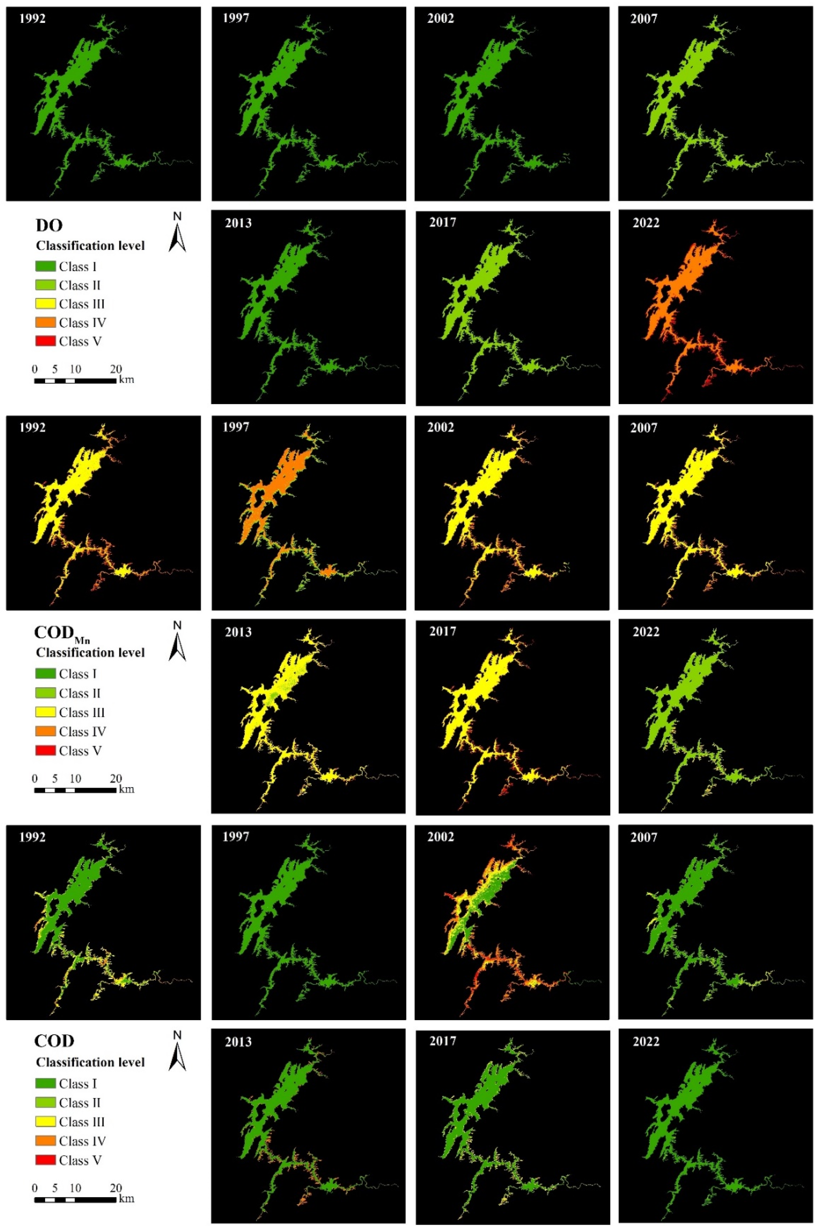
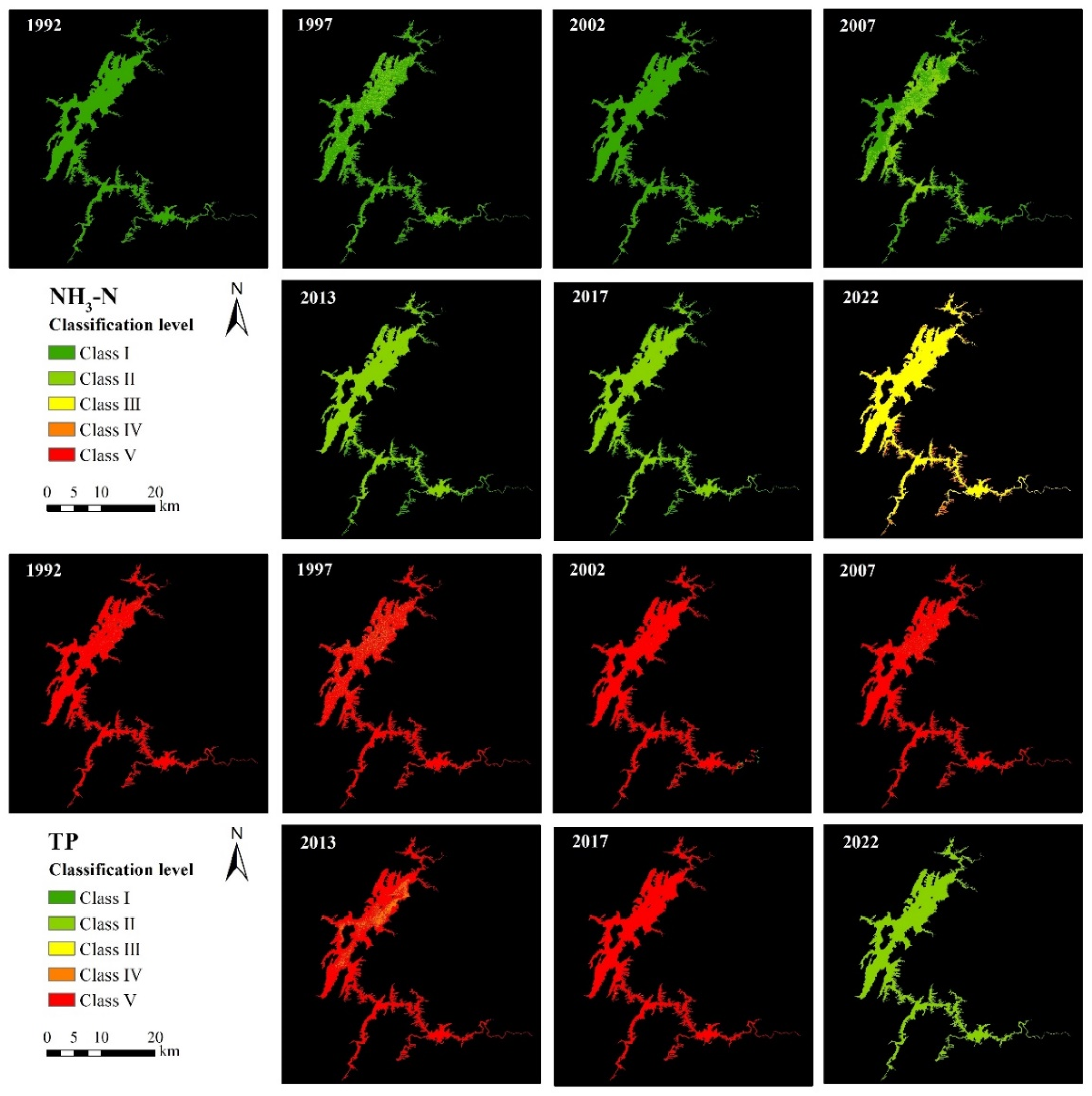
3.1. Inversion Results of Water Quality Variables

This study established remote sensing inversion models for DO, COD_Mn, COD, NH₃-N, and TP within the Dongjiang Lake. By utilizing satellite remote sensing data (with less than 10% cloud content) every five years from 1992 to 2022, we drew spatial distribution maps of DO, COD_Mn, COD, NH₃-N, and TP (Figure 2).

Based on the inversion results of each water quality parameter, we counted the annual average area proportion of the five water quality parameters that were under the Class I-V standard from 1992 to 2022 (every five years) according to the Environmental Quality Standards of Surface Water in

Table 8. Comparison of area proportion changes in five water quality parameters every five years from 1992 to 2022 based on five standards of Environmental Quality Standards of Surface Water.

Year	Parameter	Class I	Class II	Class III	Class IV	Class V
1992	DO	100.00%	0.00%	0.00%	0.00%	0.00%
	CODMn	0.00%	0.00%	70.94%	23.16%	5.90%
	COD	67.07%	0.00%	27.21%	4.45%	1.28%
	NH3-N	99.98%	0.02%	0.00%	0.00%	0.00%
	TP	0.00%	0.00%	0.08%	1.61%	98.30%
1997	DO	100.00%	0.00%	0.00%	0.00%	0.00%
	CODMn	0.00%	27.59%	8.08%	64.19%	0.14%
	COD	98.81%	0.00%	0.39%	0.47%	0.33%
	NH3-N	82.57%	17.39%	0.03%	0.01%	0.00%
	TP	0.00%	0.01%	0.62%	9.63%	89.74%
2002	DO	99.95%	0.01%	0.00%	0.01%	0.03%
	CODMn	0.11%	0.29%	74.72%	21.95%	2.93%
	COD	28.19%	0.00%	25.42%	38.75%	7.63%
	NH3-N	99.85%	0.15%	0.00%	0.00%	0.00%
	TP	0.33%	0.01%	0.05%	0.21%	99.40%
2007	DO	100.00%	0.00%	0.00%	0.00%	0.00%
	CODMn	0.00%	1.27%	79.80%	15.12%	3.80%
	COD	74.05%	0.00%	22.23%	2.72%	0.99%
	NH3-N	65.83%	34.13%	0.03%	0.00%	0.00%
	TP	0.00%	0.00%	0.02%	1.97%	98.01%
2013	DO	99.86%	0.14%	0.00%	0.00%	0.00%
	CODMn	0.00%	5.04%	86.72%	4.09%	4.16%
	COD	84.22%	0.00%	0.66%	14.60%	0.52%
	NH3-N	24.04%	75.94%	0.01%	0.00%	0.00%
	TP	0.00%	0.00%	0.00%	9.96%	90.04%
2017	DO	99.99%	0.01%	0.00%	0.00%	0.00%
	CODMn	0.00%	0.45%	80.07%	8.98%	10.50%
	COD	79.35%	0.00%	17.86%	1.70%	1.09%
	NH3-N	26.92%	73.07%	0.00%	0.00%	0.00%
	TP	0.00%	0.00%	0.00%	0.17%	99.82%
2022	DO	0.00%	0.00%	0.00%	78.99%	21.01%
	CODMn	0.00%	88.04%	10.51%	1.45%	0.00%
	COD	99.66%	0.00%	0.34%	0.00%	0.00%
	NH3-N	0.00%	0.45%	86.80%	12.20%	0.54%
	TP	0.00%	100.00%	0.00%	0.00%	0.00%

to evaluate the water quality of Dongjiang Lake as a whole.

According to the results in Table 8, it can be seen that from 1992 to 2017, the DO in the watershed was under Class I and Class II standards, but in 2022, the DO in the watershed was reduced to Class IV and Class V standards, which accounted for 78.99% and 21.01%, respectively. And the Class V standards were mainly located in the northeastern and southeastern parts of the drainage systems, which were adjacent to the land.

From 1992 to 2017, more than 70% of COD_Mn was of Class III, IV, and V standards, and in 2022, the area proportion under Class I and II standards reached 88.04%, and the area proportion under Class V standards was reduced to 0%. The quality of COD_Mn was improved overall.

Over the past 30 years, the COD has shown a trend of deterioration followed by improvement. The percentage of the Class I standard area for this parameter decreased from 98.81% to 28.19% in 1997–2002 but continued to improve to 99.66% over the following 20 years. Supported by the national policy, the government has strengthened the management of wastewater discharges, which effectively reduces the amount of organic waste discharged by industry, agriculture, and municipalities.

From 1992 to 2022, the share of Class I zones for the NH₃-N decreased from 99.98% to 0%, with the largest decrease of 41.79% from 2007 to 2013. More than 90% of the NH₃-N in the watershed decreased from Class I and Class II standards to Class III and Class IV standards. Over the past 30 years, the continuous increase in NH₃-N in Dongjiang Lake had a significant impact on the water quality.

From 1992 to 2017, more than 90% of the TP area was under the Class V standard, indicating that the TP concentration in the water body during the period was large and the water body eutrophication was serious. It posed a certain threat to the watershed ecosystem and human health. By 2022, TP improved to Class II standards due to the effective national environmental policies and regulations, which improved wastewater treatment facilities, controlled industrial wastewater discharges, and reduced exogenous nutrient inputs.

3.2. WQI Calculation Results

Based on the inversion results of the five water quality parameters, the WQI results for 1992–2022 (every five years) were calculated by the WQI formula (Figure 3).

The mean value of WQI in each map was calculated, and the ratio of the area with WQI in different classes to the total area in Figure 3 is counted in

Table 9. WQI means and its share in each category.

Year	WQI Means	WQI Class
		Class I	Class II	Class III	Class IV	Class V	Sub-Class V
1992	4.5945	0.00%	0.00%	16.15%	29.78%	32.54%	21.53%
1997	3.9695	0.00%	0.01%	5.68%	92.68%	0.62%	1.01%
2002	5.2784	0.00%	0.00%	0.02%	22.75%	26.58%	50.65%
2007	4.3345	0.00%	0.00%	27.40%	37.15%	10.03%	25.41%
2013	2.9708	0.00%	14.23%	78.74%	4.36%	1.03%	1.63%
2017	3.6886	0.00%	0.00%	74.10%	3.85%	1.16%	20.90%
2022	3.1000	0.96%	89.35%	8.42%	1.25%	0.01%	0.00%

.

From the results in Figure 3 and Table 9, it can be seen that the WQI of Dongjiang Lake decreased from 4.5945 to 2.1000 in 1992–2022, a decrease close to 60%, and improved from Class IV to Class II. Among them, 21.53% of the area in 1992 was Sub-Class V, mainly distributed in the western and southeastern parts of the water system. In 1997, the overall water quality improved; more than 90% of the area was a Class IV water body, and only 1.01% of the water body was in Class V. Due to the development of industrialization and urbanization, industrial wastewater discharges and agricultural pollution had a poor impact on water quality, and the water quality of Dongjiang Lake was at its worst in 2002, with more than 70% of the area being Class V and Sub-Class V. In 2007, water quality conditions slightly improved, but there was still 25.41% of the water body in the Sub-Class V water body. And from the aspect of spatial distribution, the central of the watershed significantly improved, and the pollution of the water body was controlled. In 2013, the WQI fell to 2.9708, and Class II and Class III accounted for more than 90%. The water quality gradually recovered to a good state, with only 2.66% in Class V and Sub-Class V. Compared to 2013, the water quality in 2017 relatively deteriorated, with 20.90% of the water body classified as Sub-Class V, and this was found in areas where the water body bordered the land. This is due to the large-scale tourism development with the Dongjiang Lake, where the passenger flow has increased dramatically, which had a negative impact on the water quality. In 2022, affected by the epidemic, the tourism industry suffered a certain blow; the flow of passengers in scenic spots decreased, coupled with the control of industrial and agricultural sewage discharges, and the water quality gradually recovered, with more than 90% being of Class I and Class II. People could drink cleaner and safer water, reducing the threat of the water body to the ecosystem.

In general, the water quality of Dongjiang Lake has shown a trend of gradual improvement during the past 30 years, but this change is still unstable. In terms of overall spatial distribution, water bodies bordering land are more vulnerable to pollution. The water quality of Dongjiang Lake is affected by industry, agriculture, tourism, and other factors. There is still a need to strictly control wastewater discharges, enhance environmental education for residents and tourists, and minimize the negative impacts of development in various sectors on water quality.

3.3. Result of Spatial and Temporal Dynamic Coupling between Water Quality and LUCC

3.3.1. Land Use Classification Results

This study employed the RF method to classify the land in the Dongjiang Lake watershed into the following six categories: grassland, arable land, unused land, forest land, water bodies, and construction land (Figure 4) and counted the area proportion of each land use from 1992 to 2022 (

Table 10. Each land use proportion from 1992 to 2022 (every 5 years) based on RF.

Year	Area/Proportion	Land Use
		Forest Land	Arable Land	Grassland	Water Bodies	Construction Land	Unused Land
1992	Area (km2)	4147.61	372.87	4.19	100.14	6.93	9.09
	Proportion (%)	89.37%	8.03%	0.09%	2.16%	0.15%	0.20%
1997	Area (km2)	4139.48	373.65	3.80	103.73	8.04	12.13
	Proportion (%)	89.20%	8.05%	0.08%	2.24%	0.17%	0.26%
2002	Area (km2)	4115.61	396.22	3.82	104.12	10.08	10.99
	Proportion (%)	88.68%	8.54%	0.08%	2.24%	0.22%	0.24%
2007	Area (km2)	4123.13	388.67	4.59	103.78	11.96	8.71
	Proportion (%)	88.84%	8.37%	0.10%	2.24%	0.26%	0.19%
2013	Area (km2)	4093.91	412.06	5.55	104.01	18.08	7.21
	Proportion (%)	88.22%	8.88%	0.12%	2.24%	0.39%	0.16%
2017	Area (km2)	4061.32	441.44	6.28	102.92	22.39	6.49
	Proportion (%)	87.51%	9.51%	0.14%	2.22%	0.48%	0.14%
2022	Area (km2)	4048.69	450.35	6.09	102.49	26.36	6.87
	Proportion (%)	87.24%	9.70%	0.13%	2.21%	0.57%	0.15%

).

As shown in Figure 4 and Table 10, from 1992 to 2022, each category in the Dongjiang Lake Watershed experienced changes in spatial distribution. Forest land was widely distributed and mainly distributed in the central part of Dongjiang Lake Watershed. Forest land decreased in most regions, with a relatively large reduction in area. Xingning Township, Qingjiang Township, Yaogangxian Township, Wenming Township, and Luyang Township were the main regions where the forest land area decreased. Arable land was mainly concentrated in the south-western, north-western, and south-eastern parts of the Dongjiang Lake Watershed. Luyang Township, Quanshui Township, Daping Township, and Jingpo Township had a large area of arable land, the main source of which was the conversion of forest land into arable land. And the trend of expansion was to the periphery of the original arable land. Construction land was mainly located in Xingning Town, Luyang Town, and Oujiang Town in the watershed, and its area increased significantly. The main sources of the area increase were forest land and arable land. Over the past 30 years, the prosperity of tourism in Dongjiang Lake has led to an increase in the demand for construction land in the surrounding regions, including hotels, scenic facilities, and transport infrastructure. And the expansion of construction land in Luyang Town, Oujiang Town, and other regions was mainly driven by the urbanization and expansion of Rucheng County and Guidong County, as well as the transfer of farmers to towns and cities, the development of the rural economy, and the establishment of infrastructures. Grassland and unused land had only a small distribution in the township, but the area was small and not very variable compared to other land types. Overall, the three land categories of forest land, arable land, and construction land in the Dongjiang Lake Watershed changed the most from 1992 to 2022, while the rest of the land categories changed relatively little.

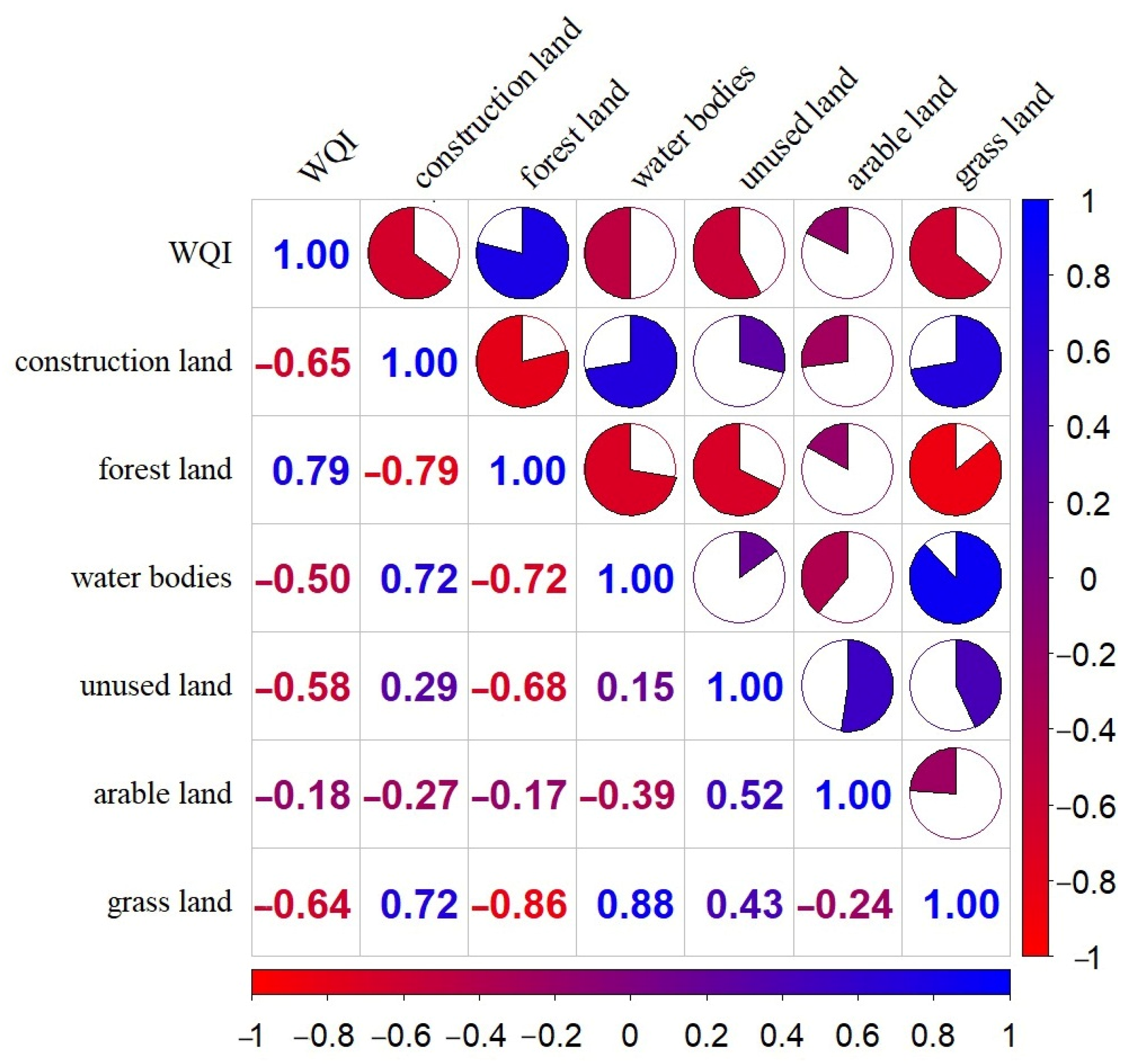
3.3.2. WQI and LUCC Coupling Results

The correlation analysis of LUCC and WQI ensures that the coupled model focuses on the most meaningful interactions between the two variables. Analysis improves the accuracy and reliability of the model, reduces the potential for errors and uncertainties in the coupling process, minimizes noise and extraneous information, and enhances model performance. This study utilized six primary land use types, including arable land, forest land, grassland, water bodies, construction land, and unused land, as independent variables to establish a mathematical statistical model. The dependent variable was the WQI. Pearson correlation analyses were conducted on the variables, and the results are presented in Figure 5.

Based on the fitting results of the coupled model between WQI and LUCC in Dongjiang Lake Watershed, the R², MAE, and RMSE of each model were calculated (Figure 6) to verify and compare the accuracy of each model.

Figure 6 shows that the polynomial model has a higher fitting accuracy than the machine learning regression model. The cubic polynomial in five variables has an R² of 0.9950, an RMSE of 0.0970, and an MAE of 0.0470, with the best fitting accuracy among all the regression models. In comparison, the cubic polynomial in four variables has slightly lower R² (0.9530), RMSE (0.2870), and MAE (0.1760), but it is 37.50% simpler than the cubic polynomial in five variables, making it more applicable and suitable.

Combining the accuracy and applicability of the model, the study established a cubic polynomial in the four variables model with grassland, forest land, construction land, and unused land as the independent variables and WQI as the dependent variable to form a spatial-temporal dynamic coupling model of water quality and LUCC in the Dongjiang Lake Watershed. Its specific form is as follows:

$$\begin{array}{cc}\hfill WQI=3.976+& 712.3\times G-8.942\times F-498.1\times C-1687.0\times U-1596.0\times G\times F-885.8\times G\times C\hfill \\ & +4986.0\times G\times U+1099.0\times F\times C+3774.0\times F\times U+6992.0\times C\times U-3009.0\times G^2\hfill \\ & +5.028\times F^2+2424.0\times C^2+5309.0\times U^2+756.2\times F\times G\times C-5451.0\times F\times G\times U\hfill \\ & -7773.0\times F\times C\times U+3465.0\times F\times G^2+2789.0\times C\times G^2-3048.0\times U\times G^2\hfill \\ & +894.7\times G\times F^2-605.3\times C\times F^2-2113.0\times U\times F^2-875.7\times G\times C^2-2700.0\times F\times C^2\hfill \\ & -13810.0\times U\times C^2-11380.0\times G\times U^2-5676.0\times F\times U^2-17500.0\times C\times U^2\hfill \\ & +2272.0\times G^3-1702.0\times C^3-6959.0\times U^3\hfill \end{array}$$

(13)

where $G$ represents the area proportion of grassland, $F$ represents the area proportion of forest land, $C$ represents the area proportion of construction land and $U$ represents the area proportion of unused land.

4. Discussion and Conclusions

LUCC affects nutrient cycling in watersheds, particularly the availability and transport of nitrogen and phosphorus [43], and thus, is a major driver of spatio-temporal changes in water quality [44]. As a non-renewable and important resource on earth, the protection and management of water quality is paramount. Rapid and drastic LUCC severely affects the water quality [45]. For the Dongjiang Lake Watershed, an important freshwater resource area, the spatial and temporal dynamic coupling relationship between its water quality and LUCC is of great significance for water quality management and environmental protection [46].

Remote sensing satellites offer cost-effective and wide-coverage-standardized monitoring data with a long time series [47]. However, the use of remote sensing data to explore the coupling relationship between water quality and LUCC is plagued [48] by problems such as the difficulty of capturing small-scale features and processes, time-consuming data processing, large errors in the estimation of water quality parameters, and poor compatibility between remote sensing and ground data [49]. This study analyzed measured data in the Dongjiang Lake Watershed to identify key water quality parameters, including DO, COD_Mn, COD, NH₃-N, and TP [26]. According to the principle that different water quality parameters have different reflectance characteristics on multispectral or hyperspectral images, the optimal band combinations for the inversion of DO, COD_Mn, COD, NH3-N, and TP were determined by Pearson correlation analysis. The measured data were combined with cross-section monitoring to assess accuracy. Multiple stepwise regression analysis was then employed to determine the inverse models for each of the five parameters. Then, we calculated the WQI of the watershed to carry out systematic and objective evaluation. The five parameters of water quality evaluation chosen by the study are in accordance with the actual characteristics of Dongjiang Lake Watershed and its water quality, which is scientifically guided and practically applicable for water quality prevention and control in the region.

Based on the spatial and temporal dynamic patterns of water quality and land use in Dongjiang Lake Watershed, this study constructed a coupled model of WQI and LUCC in the region and quantified their relationship. Based on the spatio-temporal dynamic results of water quality and land use in the study area during 1992–2022, the deep learning regression model and polynomial regression model were used to quantitatively explore the coupling relationship between WQI and LUCC in the watershed. The cubic polynomial in the four variables model with grassland, forest land, construction land, and unused land as independent variables and comprehensive water quality identification index being a dependent variable was proposed as the spatial-temporal dynamic coupling model of water quality and LUCC in Dongjiang Lake Watershed. The accuracy of the model was compared using R², MAE, and RMSE, with R² = 0.9530, MAE = 0.2870, and RMSE = 0.1760. The cubic polynomial in the four variables model can express the effect of LUCC on WQI through multiple interaction terms, which can consider the effect of different land use types on water quality more comprehensively. A high R² value indicates that the model can adequately explain the relationship between WQI and LUCC, and low RMSE and MAE values indicate that the model has a lower error between the predicted and real values and that the model can predict the changes in WQI better. The relationship between water quality index (WQI) and land use change (LUCC) is usually non-linear, and the cubic polynomial in the four variables model can effectively capture these complex non-linear relationships and, thus, predict the changes in WQI more accurately. The model can accurately reflect the coupled relationship between water quality and land use/cover change in the study area, providing a good database for accurately predicting future trends in water quality changes and for rational planning and management of water resources.

This study analyzed the coupling between LUCC and water quality from a quantitative perspective and explored the relationship and interactions between water quality and LUCC by coupling water quality and land use/cover changes (LUCCs). The proposed method can effectively help to deepen our understanding of the driving mechanisms behind the water quality changes caused by LUCC. Further studies can combine water quality modeling with climate change modeling to investigate the long-term impacts of climate change on water quality in the Dongjiang Lake Watershed. By simulating water quality changes under different climate scenarios, possible future trends in water quality changes can be predicted, and corresponding water resource management and protection strategies can be proposed.

References

1. John, V.; Jain, P.; Rahate, M.; Labhasetwar, P. Assessment of deterioration in water quality from source to household storage in semi-urban settings of developing countries. Environ. Monit. Assess. 2014, 186, 725–734. [Google Scholar] [CrossRef] [PubMed]
2. Scanlon, B.R.; Jolly, I.; Sophocleous, M.; Zhang, L. Global impacts of conversions from natural to agricultural ecosystems on water resources: Quantity versus quality. Water Resour. Res. 2007, 43. [Google Scholar] [CrossRef]
3. Todd, A.S.; Manning, A.H.; Verplanck, P.L.; Crouch, C.; McKnight, D.M.; Dunham, R. Climate-change-driven deterioration of water quality in a mineralized watershed. Environ. Sci. Technol. 2012, 46, 9324–9332. [Google Scholar] [CrossRef]
4. Horton, R.K. An index number system for rating water quality. J. Water Pollut. Control Fed. 1965, 37, 300–306. [Google Scholar]
5. Wu, Z.; Zhang, D.; Cai, Y.; Wang, X.; Zhang, L.; Chen, Y. Water quality assessment based on the water quality index method in Lake Poyang: The largest freshwater lake in China. Sci. Rep. 2017, 7, 17999. [Google Scholar] [CrossRef]
6. Singh, K.P.; Malik, A.; Sinha, S. Water quality assessment and apportionment of pollution sources of Gomti river (India) using multivariate statistical techniques—A case study. Anal. Chim. Acta 2005, 538, 355–374. [Google Scholar] [CrossRef]
7. Mir, R.A.; Gani, K.M. Water quality evaluation of the upper stretch of the river Jhelum using multivariate statistical techniques. Arab. J. Geosci. 2019, 12, 1–19. [Google Scholar] [CrossRef]
8. Huang, J.; Gao, J.; Zhang, Y. Eutrophication prediction using a markov chain model: Application to lakes in the Yangtze River basin, China. Environ. Model. Assess. 2016, 21, 233–246. [Google Scholar] [CrossRef]
9. Wu, N.; Schmalz, B.; Fohrer, N. Development and testing of a phytoplankton index of biotic integrity (P-IBI) for a German lowland river. Ecol. Indic. 2012, 13, 158–167. [Google Scholar] [CrossRef]
10. Şener, Ş.; Şener, E.; Davraz, A. Evaluation of water quality using water quality index (WQI) method and GIS in Aksu River (SW-Turkey). Sci. Total Environ. 2017, 584, 131–144. [Google Scholar] [CrossRef]
11. Mwaijengo, G.N.; Msigwa, A.; Njau, K.N.; Brendonck, L.; Vanschoenwinkel, B. Where does land use matter most? Contrasting land use effects on river quality at different spatial scales. Sci. Total Environ. 2020, 715, 134825. [Google Scholar] [CrossRef] [PubMed]
12. Kuemmerlen, M.; Schmalz, B.; Guse, B.; Cai, Q.; Fohrer, N.; Jähnig, S.C. Integrating catchment properties in small scale species distribution models of stream macroinvertebrates. Ecol. Model. 2014, 277, 77–86. [Google Scholar] [CrossRef]
13. Kulmatov, R. Problems of sustainable use and management of water and land resources in Uzbekistan. J. Water Resour. Prot. 2014, 2014, 42350. [Google Scholar] [CrossRef]
14. Al-Mutairi, N.; Abahussain, A.; El-Battay, A. Spatial and temporal characterizations of water quality in Kuwait Bay. Mar. Pollut. Bull. 2014, 83, 127–131. [Google Scholar] [CrossRef] [PubMed]
15. Wu, Z.; Wang, X.; Chen, Y.; Cai, Y.; Deng, J. Assessing river water quality using water quality index in Lake Taihu Basin, China. Sci. Total Environ. 2018, 612, 914–922. [Google Scholar] [CrossRef] [PubMed]
16. Ritchie, J.C.; Zimba, P.V.; Everitt, J.H. Remote sensing techniques to assess water quality. Photogramm. Eng. Remote Sens. 2003, 69, 695–704. [Google Scholar] [CrossRef]
17. Topp, S.N.; Pavelsky, T.M.; Jensen, D.; Simard, M.; Ross, M.R. Research trends in the use of remote sensing for inland water quality science: Moving towards multidisciplinary applications. Water 2020, 12, 169. [Google Scholar] [CrossRef]
18. Najafzadeh, M.; Basirian, S. Evaluation of River Water Quality Index Using Remote Sensing and Artificial Intelligence Models. Remote Sens. 2023, 15, 2359. [Google Scholar] [CrossRef]
19. Vignolo, A.; Pochettino, A.; Cicerone, D. Water quality assessment using remote sensing techniques: Medrano Creek, Argentina. J. Environ. Manag. 2006, 81, 429–433. [Google Scholar] [CrossRef]
20. Najafzadeh, M.; Homaei, F.; Farhadi, H. Reliability assessment of water quality index based on guidelines of national sanitation foundation in natural streams: Integration of remote sensing and data-driven models. Artif. Intell. Rev. 2021, 54, 4619–4651. [Google Scholar] [CrossRef]
21. Mo, W.; Zhao, Y.; Yang, N.; Xu, Z.; Zhao, W.; Li, F. Effects of climate and land use/land cover changes on water yield services in the Dongjiang Lake Basin. ISPRS Int. J. Geo-Inf. 2021, 10, 466. [Google Scholar] [CrossRef]
22. Cao, F.; Qin, P.; Lu, S.; He, Q.; Wu, F.; Sun, H.; Wang, L.; Li, L. Measurement of volatile organic compounds and associated risk assessments through ingestion and dermal routes in Dongjiang Lake, China. Ecotoxicol. Environ. Saf. 2018, 165, 645–653. [Google Scholar] [CrossRef] [PubMed]
23. Lyu, L.; Bi, S.; Yang, Y.; Zheng, D.; Li, Q. Effects of vegetation distribution and landscape pattern on water conservation in the Dongjiang River basin. Ecol. Indic. 2023, 155, 111017. [Google Scholar] [CrossRef]
24. Jiang, J.; Wang, Z.; Lai, C.; Wu, X.; Chen, X. Climate and landuse change enhance spatio-temporal variability of Dongjiang river flow and ammonia nitrogen. Sci. Total Environ. 2023, 867, 161483. [Google Scholar] [CrossRef] [PubMed]
25. Mo, W.; Yang, N.; Zhao, Y.; Xu, Z. Impacts of land use patterns on river water quality: The case of Dongjiang Lake Basin, China. Ecol. Inform. 2023, 75, 102083. [Google Scholar] [CrossRef]
26. Dong, L.; Gong, C.; Huai, H.; Wu, E.; Lu, Z.; Hu, Y.; Li, L.; Yang, Z. Retrieval of Water Quality Parameters in Dianshan Lake Based on Sentinel-2 MSI Imagery and Machine Learning: Algorithm Evaluation and Spatiotemporal Change Research. Remote Sens. 2023, 15, 5001. [Google Scholar] [CrossRef]
27. Kannel, P.R.; Lee, S.; Lee, Y.-S.; Kanel, S.R.; Khan, S.P. Application of water quality indices and dissolved oxygen as indicators for river water classification and urban impact assessment. Environ. Monit. Assess. 2007, 132, 93–110. [Google Scholar] [CrossRef] [PubMed]
28. Zhang, S.; Zhang, H. Anthropogenic impact on long-term riverine CODMn, BOD, and nutrient flux variation in the Pearl River Delta. Sci. Total Environ. 2023, 859, 160197. [Google Scholar] [CrossRef] [PubMed]
29. Liu, L.; Cao, T.-t.; Wang, X.-d.; Dandan, Z.; Cui, C.-W. Spatio-temporal variability and water quality assessment of the Mudan River Watershed, Northern China: Principal component analysis and water quality index. Desalination Water Treat 2021, 238, 38–48. [Google Scholar] [CrossRef]
30. Rodríguez-López, L.; Alvarez, D.; Bustos Usta, D.; Duran-Llacer, I.; Bravo Alvarez, L.; Fagel, N.; Bourrel, L.; Frappart, F.; Urrutia, R. Chlorophyll-a Detection Algorithms at Different Depths Using In Situ, Meteorological, and Remote Sensing Data in a Chilean Lake. Remote Sens. 2024, 16, 647. [Google Scholar] [CrossRef]
31. Johnes, P.; Moss, B.; Phillips, G. The determination of total nitrogen and total phosphorus concentrations in freshwaters from land use, stock headage and population data: Testing of a model for use in conservation and water quality management. Freshwat. Biol. 1996, 36, 451–473. [Google Scholar] [CrossRef]
32. Said, S.; Khan, S.A. Remote sensing-based water quality index estimation using data-driven approaches: A case study of the Kali River in Uttar Pradesh, India. Environ. Dev. Sustain. 2021, 23, 18252–18277. [Google Scholar] [CrossRef]
33. Zeng, J.; Liu, Z.; Liu, X.; Zhang, L.; Zhang, J.; Zeng, Y. The Spatiotemporal Variations and Potential Causes of Water Quality of Headwaters of Dongjiang River, Southeastern China. Sustainability 2023, 15, 6455. [Google Scholar] [CrossRef]
34. Uddin, M.G.; Nash, S.; Olbert, A.I. A review of water quality index models and their use for assessing surface water quality. Ecol. Indic. 2021, 122, 107218. [Google Scholar] [CrossRef]
35. Poonam, T.; Tanushree, B.; Sukalyan, C. Water quality indices-important tools for water quality assessment: A review. Int. J. Adv. Chem. 2013, 1, 15–28. [Google Scholar]
36. Liu, W.; Liu, J.; Kuang, W.; Ning, J. Examining the influence of the implementation of Major Function-oriented Zones on built-up area expansion in China. J. Geogr. Sci. 2017, 27, 643–660. [Google Scholar] [CrossRef]
37. Singh, S.K.; Mustak, S.; Srivastava, P.K.; Szabó, S.; Islam, T. Predicting spatial and decadal LULC changes through cellular automata Markov chain models using earth observation datasets and geo-information. Environ. Process. 2015, 2, 61–78. [Google Scholar] [CrossRef]
38. Hasan, S.S.; Zhen, L.; Miah, M.G.; Ahamed, T.; Samie, A. Impact of land use change on ecosystem services: A review. Environ. Dev. 2020, 34, 100527. [Google Scholar] [CrossRef]
39. Abd Ellah, R.G. Water resources in Egypt and their challenges, Lake Nasser case study. Egypt. J. Aquat. Res. 2020, 46, 1–12. [Google Scholar] [CrossRef]
40. Zhang, X.; Chen, P.; Han, Y.; Chang, X.; Dai, S. Quantitative analysis of self-purification capacity of non-point source pollutants in watersheds based on SWAT model. Ecol. Indic. 2022, 143, 109425. [Google Scholar] [CrossRef]
41. Breiman, L. Random forests. Mach. Learn. 2001, 45, 5–32. [Google Scholar] [CrossRef]
42. Leong, W.C.; Bahadori, A.; Zhang, J.; Ahmad, Z. Prediction of water quality index (WQI) using support vector machine (SVM) and least square-support vector machine (LS-SVM). Int. J. River Basin Manag. 2021, 19, 149–156. [Google Scholar] [CrossRef]
43. Belay, H.; Melesse, A.M.; Tegegne, G. Scenario-Based Land Use and Land Cover Change Detection and Prediction Using the Cellular Automata–Markov Model in the Gumara Watershed, Upper Blue Nile Basin, Ethiopia. Land 2024, 13, 396. [Google Scholar] [CrossRef]
44. Lang, F.; Liang, Y.; Li, S.; Cheng, Z.; Li, G.; Guo, Z. Spatio-Temporal Patterns of Land Use and Cover Change in the Lancang–Mekong River Basin during 2000–2020. Land 2024, 13, 305. [Google Scholar] [CrossRef]
45. Al-Taei, A.I.; Alesheikh, A.A.; Darvishi Boloorani, A. Land Use/Land Cover Change Analysis Using Multi-Temporal Remote Sensing Data: A Case Study of Tigris and Euphrates Rivers Basin. Land 2023, 12, 1101. [Google Scholar] [CrossRef]
46. Wang, Y.; Yang, F.; He, F. Spatiotemporal Characteristics of Land Cover Change in the Yellow River Basin over the Past Millennium. Land 2024, 13, 260. [Google Scholar] [CrossRef]
47. Bygate, M.; Ahmed, M. Monitoring Water Quality Indicators over Matagorda Bay, Texas, Using Landsat-8. Remote Sens. 2024, 16, 1120. [Google Scholar] [CrossRef]
48. Jang, W.; Kim, J.; Kim, J.H.; Shin, J.-K.; Chon, K.; Kang, E.T.; Park, Y.; Kim, S. Evaluation of Sentinel-2 Based Chlorophyll-a Estimation in a Small-Scale Reservoir: Assessing Accuracy and Availability. Remote Sens. 2024, 16, 315. [Google Scholar] [CrossRef]
49. Jakovljevic, G.; Álvarez-Taboada, F.; Govedarica, M. Long-Term Monitoring of Inland Water Quality Parameters Using Landsat Time-Series and Back-Propagated ANN: Assessment and Usability in a Real-Case Scenario. Remote Sens. 2024, 16, 68. [Google Scholar] [CrossRef]
Figure 1. Geographical location of the study area in Dongjiang Lake Watershed.
Land 13 00861 g001
Figure 2. Inversion results of DO, CODMn, COD, NH3-N, and TP from 1992 to 2022 (every five years).
Land 13 00861 g002aLand 13 00861 g002b
Figure 3. The WQI results from 1992 to 2022 (every five years).
Land 13 00861 g003
Figure 4. Land use classification results from 1992 to 2022 (every 5 years) based on RF. LULC in the figure means land use and land cover.
Land 13 00861 g004
Figure 5. Results of Pearson correlation analysis between land use type and WQI.
Land 13 00861 g005
Figure 6. Accuracy comparison of WQI- and LUCC-coupled models based on R2, MAE, and RMSE evaluation indexes. C represents cubic polynomial, Q represents quadratic polynomial, L represents Linear Polynomial, A represents Quartic Polynomial, and I represents Quintic Polynomial. The use of 3 represents the polynomial in three variables, 4 represents the polynomial in four variables, and 5 represents the polynomial in five variables. So, Q-3 means Quadratic Polynomial in three variables, and the rest is the same.
Land 13 00861 g006