Article

The Spatiotemporal Variability of Soil Available Phosphorus and Potassium in Karst Region: The Crucial Role of Socio-Geographical Factors

1
College of Resources and Environment, Southwest University, Chongqing 400716, China
2
Southeast Sichuan Geological Team, Chongqing Bureau of Geology and Minerals Exploration, Chongqing 400038, China
3
College of Computer and Information Science, Southwest University, Chongqing 400716, China
*
Author to whom correspondence should be addressed.
Land 2024, 13(6), 882; https://doi.org/10.3390/land13060882
Submission received: 10 May 2024 / Revised: 13 June 2024 / Accepted: 17 June 2024 / Published: 18 June 2024
(This article belongs to the Special Issue New Insights in Soil Quality and Management in Karst Ecosystem II)

Abstract

:
The contents of soil available phosphorus (AVP) and potassium (AVK) in karstic mountainous agricultural areas have changed rapidly in recent decades. This temporal variation displays strong spatial heterogeneity due to these areas’ complex topography and anthropogenic activities. Socio-geographical factors can reflect the changes in the natural environment caused by human beings, and our objective is to enhance understanding of their role in explaining the changes of AVP and AVK. In a typical karst region (611.5 km2) with uniform soil parent material and low climatic variability, 255 topsoil samples (138 in 2012 and 117 in 2021) were collected to quantify the temporal AVP and AVK changes. Random forest (RF) and partial dependence plot analyses were conducted to investigate the responses of these changes to socio-geographical factors (distance from the nearest town center [DFT] and village density [VD]), topography, biology, and landscape pattern indexes. The mean values of AVP (48.25 mg kg−1) and AVK (357.67 mg kg−1) in 2021 were significantly (p < 0.01) higher than those in 2012 (28.84 mg kg−1 and 131.67 mg kg−1, respectively). Semi-variance analysis showed strong spatial autocorrelation for AVP and AVK, ranging from 7.29% to 10.95% and 13.31% to 10.33% from 2012 to 2021, respectively. Adding socio-geographical factors can greatly improve the explanatory power of RF modeling for AVP and AVK changes by 19% and 27%, respectively. DFT and VD emerged as the two most important variables affecting these changes, followed by elevation. These three variables all demonstrated clear nonlinear threshold effects on AVP and AVK changes. A strong accumulation of AVP and AVK was observed at DFT < 5 km and VD > 20. The AVP changes increased dramatically when the elevation ranged between 1298 m and 1390 m, while the AVK changes decreased rapidly when the elevation ranged between 1350 m and 1466 m. The interaction effects of DFT and VD with elevation on these changes were also demonstrated. Overall, this study examined the important role of socio-geographical factors and their nonlinear threshold and interaction effects on AVP and AVK changes. The findings help unravel the complex causes of these changes and thus contribute to the design of optimal soil phosphorus and potassium management strategies.

1. Introduction

Phosphorus (P) and potassium (K) are crucial elements of plant nutrition, and their deficiencies can contribute to reduced plant growth, yield, and health [1,2,3,4]. Unlike nitrogen with an atmospheric source, terrestrial plants obtain most of their P and K only from soils [5]. The portions of total P and K that are readily available for absorption by plant roots are referred to as soil available P (AVP) and soil available K (AVK) [6], which are very limited in natural soils [3,5,7]. To prevent crop P and K deficiencies, farmers in major agricultural countries (e.g., China) have been intensively applying chemical P/K fertilizers over the past decades [8,9,10]. Despite boosting crop yields, the excessive application of these fertilizers poses many ecological and economic concerns, such as resource wastage, low P/K efficiency, an unbalanced composition of soil nutrients, and P leaching [3,7,11,12,13,14]. The spatiotemporal variability of AVP and AVK in agroecosystems is determined by various environmental variables, such as natural and socio-geographical factors [1,2,3,4,7,15,16,17]. Therefore, understanding the dynamics of AVP and AVK and the factors influencing their variability in agricultural systems is important to achieve optimal soil management for crop production and environmental quality.
The effects of natural factors (e.g., topography) on soil P and K have been well documented in previous studies [1,2,3,7,15]. For example, elevation can influence the weathering of bedrock and the transport and deposition of soil P and K [1,3,18]. The spatiotemporal variability of soil P and K in agro-ecosystems can also be influenced by human beings through intentional actions (e.g., land use type and fertilization) or incidental effects (enrichment sources of P and K [e.g., rubbish dumps and manure piles]) [4]. However, except for land use types and their derived variables (e.g., landscape pattern indices), other anthropogenic factors (e.g., fertilizer, enrichment sources) are generally difficult to investigate and quantify [19,20]. By contrast, socio-geographical factors (e.g., distance from the nearest town center and village/population density), which reflect the transformation of the natural environment triggered by the productive activities of humans, can be accurately investigated and spatialized. Previous studies have also revealed the great potential of these factors in driving AVP and AVK variability [4,16,17,21,22]. For example, Turner and Hiernaux [4] and Samaké [17] found higher levels of soil P and K in fields located close to villages and attributed such findings to the large amount of agricultural inputs and net nutrient transfers from outlying areas. Population density is also positively correlated with soil K and P content [16,21,22]. Overall, socio-geographical factors have an important influence on AVP and AVK, but their relative importance compared with natural factors remains unclear. This outstanding issue might prevent an integrative understanding of the critical drivers of soil P and K dynamics in agricultural areas.
Many scholars suggest that the relationship between natural factors and soil nutrients (e.g., soil P) [2,23] and between socio-geographical factors and soil pollutants [24,25] may be nonlinear or has a threshold type. However, only a few studies have verified the nonlinear threshold effects of socio-geographical factors on soil P and K [17]. Samaké et al. [17], who identified the potential nonlinear threshold effects of socio-geographical factors on soil P and K, found that soil P and K in fallow plots do not significantly differ when the distance from the village exceeds a specific threshold (500 m and 1000 m, respectively). However, they identified these thresholds by discretizing the independent variables [17], which cannot sufficiently reflect the sudden changes in the relationship between socio-geographical factors and soil P and K [25]. Other studies suggest that the effect of one environmental factor on soil P and K is often driven by another factor [1,4,20,22]. For example, after controlling for the locational factor, the soil P content remains negatively related to the distance to the village, although the significance of such a relationship has declined [4]. Overall, socio-geographical factors may have nonlinear threshold and interaction effects on AVP and AVK. Exploring such potential effects may provide insights into the spatial variation mechanisms of soil P and K.
As the largest continuous karst region in the world, the southwest China karst region is also one of the least undeveloped areas in China [26]. To escape poverty, tobacco is widely cropped by local farmers as an important source of income. In recent years, the rapid accumulation of P and K in tobacco soils has been witnessed [27,28]. However, the influence of socio-geographical factors, as important factors characterizing anthropogenic activities, on soil P and K accumulation remains unclear. Therefore, the objectives of this study are to (1) investigate the temporal changes in AVP and AVK; (2) determine the impact of socio-geographical factors on these changes; and (3) explore the nonlinear threshold and interaction effects of socio-geographical factors on these changes. This study was conducted in a karstic sub-region (611.5 km2) with uniform soil parent material and low climatic variability. Especially, random forest (RF) modeling and partial dependence plot (PDP) analysis were employed to examine the effects of socio-geographical factors on AVK and AVK changes.

2. Materials and Methods
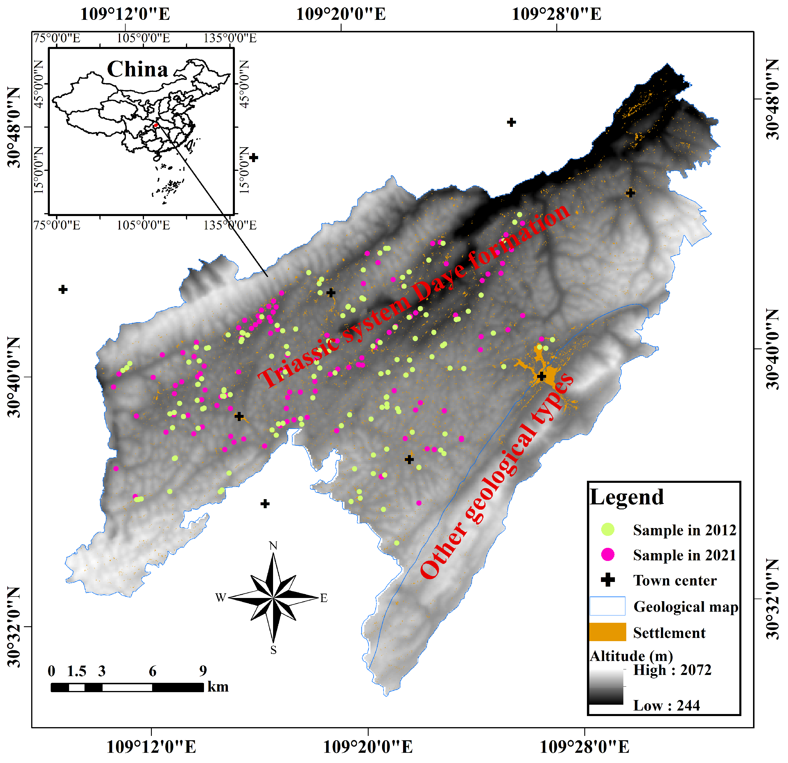
2.1. Study Area

The study area is located in the karst region of southwest China (109°9′–109°32′ E, 30°29′–30°49′ N), which covers an area of 611.5 km2 (Figure 1). This site has a typical subtropical monsoon climate with a mean temperature of 18 °C, mean annual precipitation of 1132 mm, mean annual total evaporation of 870.4 mm, relative humidity of 67%, and sunlight of 1242.6 h. The topography is mountainous, with an elevation varying between 244 m and 2072 m and a slope ranging between 0° and 75°. The Triassic system Daye formation carbonate rocks cover about 95% of the study area. The population density in the area is relatively low, at 182 person km−2, while the distribution of settlements is scattered. Planting flue-cured tobacco (Nicotiana tabacum L.) is the main source of income for local farmers. Tobacco fields are mainly distributed on both sides of the roads. The growing season for tobacco lasts from May to September, and most tobacco fields are not cropped during the other months. The amount of nitrogen fertilizer consumed in this area reaches approximately 111.45 kg ha−1 every year, while those of P and K fertilizers are 90 kg ha−1–120 kg ha−1 and 270 kg ha−1–315 kg ha−1, respectively.

2.2. Soil Sampling and Chemical Analysis

A total of 138 and 117 tobacco field topsoil (0 cm–20 cm) samples were collected from the study area in 2012 and 2021, respectively, before tobacco planting and fertilization (March). The sampling densities in 2012 and 2021 were 0.23 and 0.19 points per square kilometer, respectively. The average sampling distance in 2012 and 2021 was 0.59 km and 0.45 km, respectively. According to a highly influential review [29], the sampling density for studies within a spatial extent of 104 km2 is usually between 0.01 and 0.1 points per square kilometer. According to the recent national-scale soil surveys in China (i.e., the third national soil census), the sampling distance of the topsoil cropland samples in this area is 1 km. Therefore, the sampling densities and average sampling distances in 2012 and 2021 fall within the commonly used ranges.
The sampling sites were selected from local unique organizational units, namely, basic planting units (BPU). Each BPU consists of multiple neighboring tobacco fields with a total area exceeding 8 hectares. These BPUs are randomly dispersed across the entire study area, and our sampling activities in 2012 and 2021 encompassed all of them. Moreover, in each BPU, at least one representative tobacco field with 600 m2 to 1000 m2 was selected for sampling. The spatial location of these sites was recorded using a handheld GPS receiver, and 3 to 5 subsamples were collected and well mixed to represent the AVP and AVK information for each site. About 2 kg of the well-mixed sample was air-dried in a laboratory and then gently crushed to pass through a nylon sieve. The AVP content was determined via HCl-H2SO4 extraction and colorimetry, while the AVK content was measured via ammonium acetate extraction and colorimetry [30].

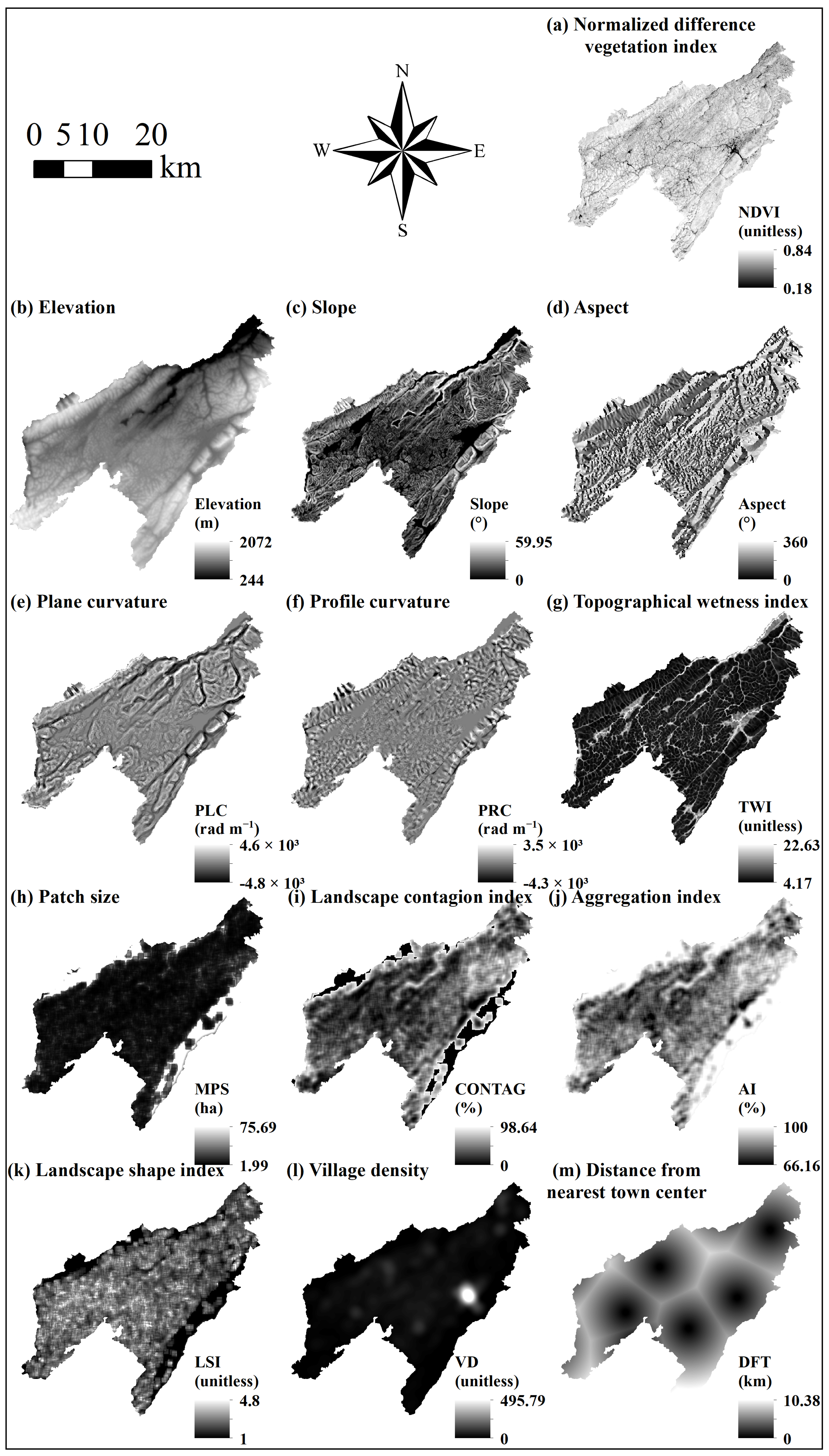
2.3. Environmental Variables

Based on classical theories (i.e., Jenny’s factorial model of soil formation and Scorpan model) [31,32] and existing studies [1,2,3,4,17,22,25,33,34,35,36], a total of 13 environmental variables representing topography, biology, landscape pattern, and socio-geographical factors were used to assess the spatiotemporal variability of AVP and AVK (Table 1 and Figure 2). All samples were obtained from the same geological formation (i.e., Triassic system Daye formation) (Figure 1). The annual temperature of sampling sites is closely related to altitude, and the soil samples received similar amounts of precipitation with a coefficient of variation (CV) of 0.05%. Consequently, geological and climatic variables were excluded from the environmental variable set.
The annual normalized difference vegetation index (NDVI) of Landsat-8 images taken from 2013 to 2021 was computed from the Google Earth Engine platform using the maximum value composite procedure [37]. In 2012, no available NDVI products from the Landsat missions were found. Specifically, the satellites from Landsat-1 to Landsat-5 ceased acquiring images in 2012. The Landsat-6 satellite launch failed. Landsat-7 products were not considered due to well-known striping issues (i.e., wedge-shaped scan-to-scan gaps). The Landsat-8 satellite had not yet been launched in 2012. The average NDVI values were calculated at a 30 m resolution.
An elevation map (ASTER GDEM v3) with a resolution of 30 m was used in this paper [38]. Six terrain indicators, namely, elevation (Ele), aspect (Asp), slope (Slp), plane curvature (PLC), profile curvature (PRC), and topographical wetness index (TWI), were calculated using SAGAGIS v7.2.0 [28].
Four classical landscape metrics, namely, mean patch size (MPS), landscape contagion index (CONTAG), aggregation index (AI), and landscape shape index (LSI), were employed to provide landscape pattern information [19,39]. A higher MPS corresponds to a larger average area of patches in the landscape, higher CONTAG and AI correspond to higher connectivity, and larger LSI corresponds to more complex landscape shapes [39]. The landscape metrics of each parcel were calculated at the landscape level using the moving window method and based on the land use map with a 30 m resolution and the FRAGSTATS 4.1 software [19,39]. The land use map, surveyed by the Chongqing Provincial Department of Land and Resources, was not open to the public. The original data for the land use map is a 1:10,000 vector file, but we only had access to the 30 m resolution raster file derived from the vector file. The optimal sliding window of 840 m was determined through extensive testing following the procedures in Liu et al. [19].
The raster maps of village density (VD) and distance from the nearest town center (DFT) were generated using the point density and near tool of ArcGIS v10.3 [40], respectively. Village vectors were derived from the land use map taken in 2016, and the town centers were determined from the land use map and the Google Earth Pro platform.

2.4. Classical Statistics

Descriptive statistical analysis (i.e., mean, median, minimum, maximum, standard deviation [SD], coefficient of variation [CV], and skewness) was performed to characterize the AVP and AVK contents and environmental variables. The independent sample t-test was applied to assess the differences in the AVP and AVK contents between the two periods after natural log transformation. All statistical analyses were conducted in SPSS v22 [41].

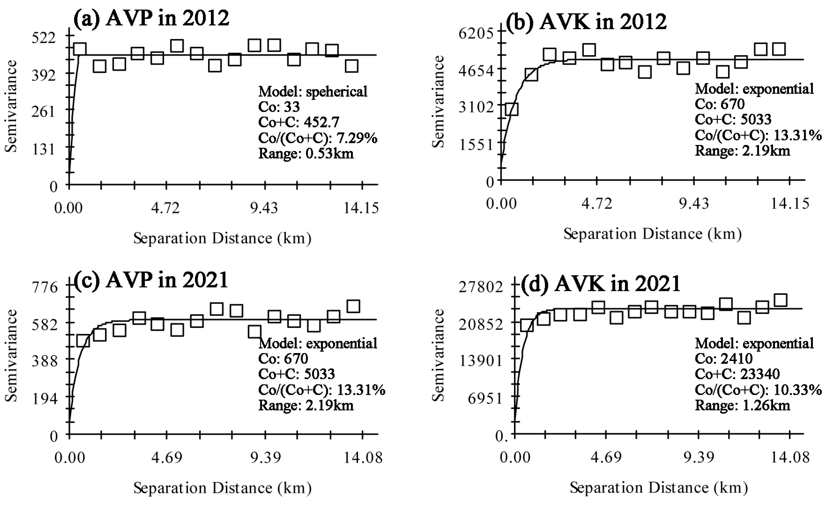
2.5. Spatiotemporal Analysis of AVP and AVK

The spatial variability of AVP and AVK in 2012 and 2021 was identified through a semi-variance analysis in GS+ 7.0 software [42]. The software automatically selects the optimal theoretical model, as indicated by the smallest residual sum of squares (RSS) and the largest coefficient of determination (R2), and the corresponding parameters, namely, nugget variance (Co), sill variance (Co + C), and range. The ratio of Co and Co + C represents the nugget effect, which is an important parameter for describing spatial autocorrelation. Nugget effects of <25%, 25%–75%, and >75% represent strong, moderate, and weak spatial autocorrelations, respectively [42]. Moreover, based on the basic parameters derived from the semi-variance analysis, the raster maps of AVP and AVK in 2012 and 2021 were produced via ordinary kriging interpolation in the geostatistical analyst tools of ArcGIS v.10.3 [40]. Using geostatistical analyst tools, the directions and ranges of the major axis and minor axis were examined, and the anisotropy ratio (the ratio of the major axis range to the minor axis range) was calculated. If the anisotropy ratio is greater than 1, it means that soil properties exhibit greater spatial variability in the major axis direction, and vice versa [43].
The maps of AVP and AVK changes were then generated by performing raster subtraction on the predictions captured in 2012 and 2021. Afterward, information on the AVP and AVK changes was extracted from the 255 samples collected in 2 years using the extract multi values to points tool in ArcGIS v.10.3 [40]. The spatial clustering of AVP and AVK changes was detected using the local indicators of spatial association (LISA) analysis developed by Anselin [38]. The following clustering patterns were identified: (i) no significant spatial dependence; (ii) high–high, high value in a high-value neighborhood; (iii) high–low, high value in a low-value neighborhood; (iv) low–high, low value in a high-value neighborhood; and (v) low–low, low value in a low-value neighborhood [28,44].

2.6. RF Modeling and Accuracy Comparison

The effects of topographical factors, landscape pattern factors, and socio-geographic factors on AVP changes and AVK changes were analyzed and compared by RF modeling. RF is a typical bagging ensemble learning model that combines the output of multiple decision trees to reach a single result [45]. RF is developed based on two important ideas, namely, the bagging method and feature randomness. In bagging, a large number of trees are built based on bootstrap sampling of training data. All tree predictions are aggregated through averaging, and these averages are taken as the final predictions. Feature randomness means that only a subset of the original covariate set is considered in the tree-splitting process. RF has two main hyperparameters, which need to be set before training. The hyperparameter “n_estimators” (the number of trees in the forest) was set to 500 since our repeated experiments showed that this was sufficient to obtain stable results. The hyperparameter “max_features” (the number of maximum features provided to each tree) was set to the default value of the square root of the total number of covariates.
Five RF models were constructed based on different combinations of environmental variables. Model-A includes NDVI and the topographic variables; Model-B includes NDVI, the topographic variables, and landscape patterns; Model-C includes NDVI, the topographic variables, and socio-geographical factors; and Model-D includes all variables. Given that the reduction in the prediction performance of Model-D for AVK and AVP changes was due to information redundancy (Section 3.3) [46], the Boruta algorithm was used to select the optimal combination of variables for Model-E. The Boruta algorithm is a popular variable selection method used in machine learning, as proposed by Kursa and Rudnicki [47]. The main steps of the Boruta algorithm are as follows: (1) enlarge the variable database and add >5 shadow attributes to each variable; (2) perform shuffle procedures on all attributes to remove correlations; (3) execute RF modeling based on the expanded data and calculate Z-scores (Equation (1)) for each attribute; (4) select variables based on Z-scores and generate a new dataset; (5) repeat the above steps until assigned criteria.
Z   scores = M e a n ( O O B a c c O O B a c c _ s h u f f l e ) S D ( O O B a c c O O B a c c _ s h u f f l e )
where OOBacc and OOBacc_shuffle are the out-of-bag accuracy of each decision tree with and without shuffle attributes, respectively. The mean and SD represent the mean and standard deviation of OOBacc-OOBacc_shuffle, respectively.
A 10-times 10-fold cross-validation (100 replications) technique was used to evaluate the five RF models. The prediction performance of these models was assessed by root mean square error (RMSE) (Equation (2)) and R2 (Equation (3)).
R M S E = 1 n i = 1 n ( x i y i ) 2
R 2 = 1 - i = 1 n ( x i y i ) 2 i = 1 n ( x i y m ) 2
where xi and yi represent the measured and predicted values of the i-th sample, respectively, n is the number of soil samples, and ym is the mean prediction values. The RF model and Boruta algorithm were developed based on the Scikit-learn and BorutaPy libraries embedded in Python v3.8, respectively.

2.7. Variable Importance and Partial Dependence Plot Analysis

The effects of environmental variables on AVP changes and AVK changes were revealed by the nodes’ impurity decrease method [45]. In 100 repetitions of each RF model, the mean values of the relative contribution of environmental variables to sAVP changes or AVK changes can be identified. The contribution of the most important variable was set to 100%, and the relative importance of the other variables was scaled.
PDP analysis was performed to visualize the complex effects of environmental variables on AVP changes and AVK changes. This method can reveal the marginal effect of one or two features on the predicted outcome of the RF model [48,49], which is accomplished in this study by a one-way PDP analysis and a two-way PDP analysis, respectively. Considering the sample set size, all samples were used for PDP analysis. PDP analysis was executed in Python v3.8.

3. Results

3.1. Descriptive Statistics

The AVP and AVK levels in 2012 and 2021 are shown in Table 2. The mean ± standard deviation of AVP in 2012 and AVP in 2021 were 28.84 ± 21.11 mg kg−1 and 48.25 ± 24.76 mg kg−1, respectively, while their mean values were 131.67 mg kg−1 (32.12 mg kg−1–371.44 mg kg−1) and 357.34 mg kg−1 (97.54 mg kg−1–782.79 mg kg−1). The distributions of AVP and AVK in 2012 and 2021 are positively skewed (right-skewed). According to the independent samples t-test, the AVP and AVK contents increased significantly (p < 0.01) by 19.41 mg kg−1 and 225.67 mg kg−1 from 2012 to 2021, respectively. As indicated by their CV, the AVP and AVK contents in these two periods exhibited high variability (CV > 35%) [50], with the variabilities in 2021 being lower than those in 2012.
The tobacco fields in the study area were distributed at high elevations (>1000 m) and in any slope direction and terrain curvature (concave or convex). The mean values of NDVI, Slp, TWI, MPS, AI, CONTAG, and LSI were 0.65, 7.55°, 10.2, 6.65 ha, 81.81%, 25.32%, and 1.73, respectively. The distances of tobacco fields from the town center ranged from 0.65 km to 7.77 km, with an average distance of 3.65 km. The village density was 29.44 ± 21.38. The distributions of NDVI, Ele, PLC, PRC, and AI are negatively skewed (left-skewed), while those of the other environmental variables are positively skewed (right-skewed). NDVI, Ele, AI, and LSI showed low variability (CV < 15%), and all other environmental variables demonstrated strong variability with CV values ranging from 37.33% to 128.78%.

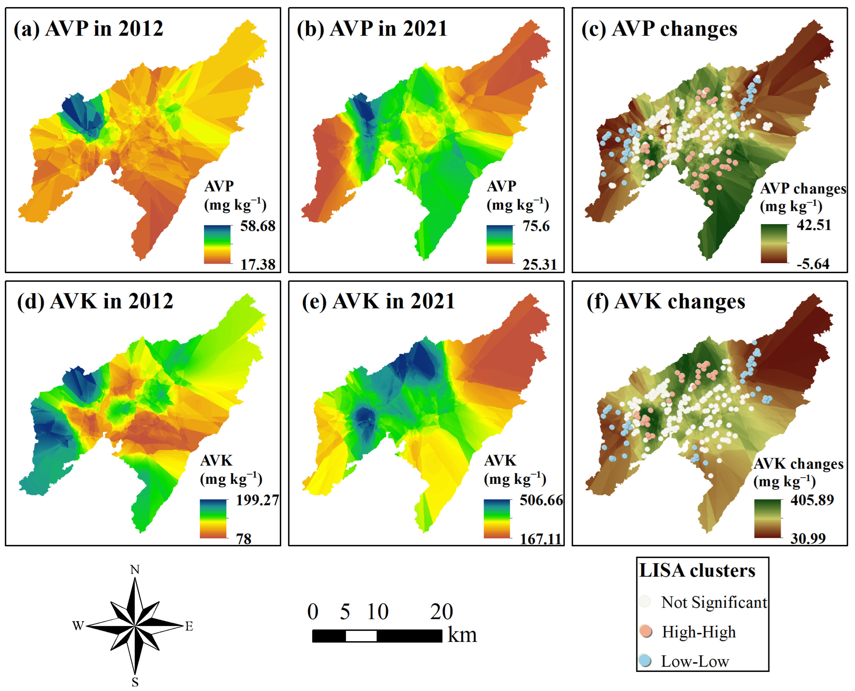
3.2. Spatio-Temporal Variability of Soil Properties

AVP2012 was optimally fitted by the spherical semi-variogram model, while AVP2021, AVK2012, and AVK2021 were best fitted by the exponential model (Figure 3 and Table S1). Following the classification described in Cambardella et al. [42], a strong spatial autocorrelation was observed in AVP2012, AVP2021, AVK2012, and AVK2021 (nugget effect [Co/(Co + C)] < 25%). The spatial autocorrelation ranges of AVP2021 exceeded those of AVP2012, thereby suggesting that the spatial distribution of the former was more homogeneous than that of the latter [42]. Similarly, compared with AVK2021, the spatial distribution of AVK2012 was more homogeneous. Besides, the anisotropy assessment results showed that the directions of the major axis were northwest-southeast, and the anisotropy ratios of AVP and AVK were all less than 1 (Table S1). This implied that AVP and AVK exhibited stronger variations in the minor axis direction (i.e., southwest-northeast), which was consistent with the topographical direction. The ranges for AVP and AVK in the two periods were greater than or close to the sampling distance, implying that our sampling system was adequate for detecting the spatial patterns of AVP and AVK [52,53,54].
The optimal parameters identified in the semi-variance analysis were employed as input parameters for ordinary kriging interpolation. The spatial distributions of AVK and AVP differed between the two periods (Figure 4a,b,d,e). For example, the AVP content in the central part of the study area was higher than that in the eastern and western parts in 2021 yet was generally similar to that in the eastern and western parts in 2012. The spatial distribution of AVP and AVK changes (Figure 4c,f) was similar in the northern, eastern, and western parts of the study area. The southern part exhibited high AVP changes and low AVK changes, while the AVP and AVK changes in the eastern and western parts predominantly displayed low–low clustering. In the southern part, a high–high clustering of AVP changes and a slight low–low clustering of AVK changes were observed.

3.3. Model Performance

Statistics on the prediction performance of all five models for AVP and AVK changes are summarized in Table 3. Using only terrain variables, Model-A explained 14% and 15% of the variance in AVP and AVK changes, respectively. Model performance was slightly improved by the addition of landscape pattern indices and significantly improved by the addition of socio-geographical factors. Model-D employed all variables to predict AVP and AVK changes and obtained R2 values of 0.36 ± 0.13 and 0.40 ± 0.11 and RMSE values of 7.34 ± 0.77 mg kg−1 and 58.91 ± 6.69 mg kg−1, respectively. Model-E obtained the best prediction performance for AVP and AVK changes, with the highest R2 of 0.41 ± 0.14 and 0.44 ± 0.13 and the lowest RMSE of 7.11 ± 0.79 mg kg−1 and 56.89 ± 6.57 mg kg−1, respectively. Among the 13 environmental variables, the Boruta algorithm retained 8 and 9 covariates for AVP and AVK changes, respectively (Table S2). NDVI, DFT, VD, Ele, Slp, PLC, and AI were retained in the prediction of AVP and AVK changes. Other variables used for predicting AVP changes included TWI in Model-E, while those used for predicting AVK changes included CONATG and Asp.

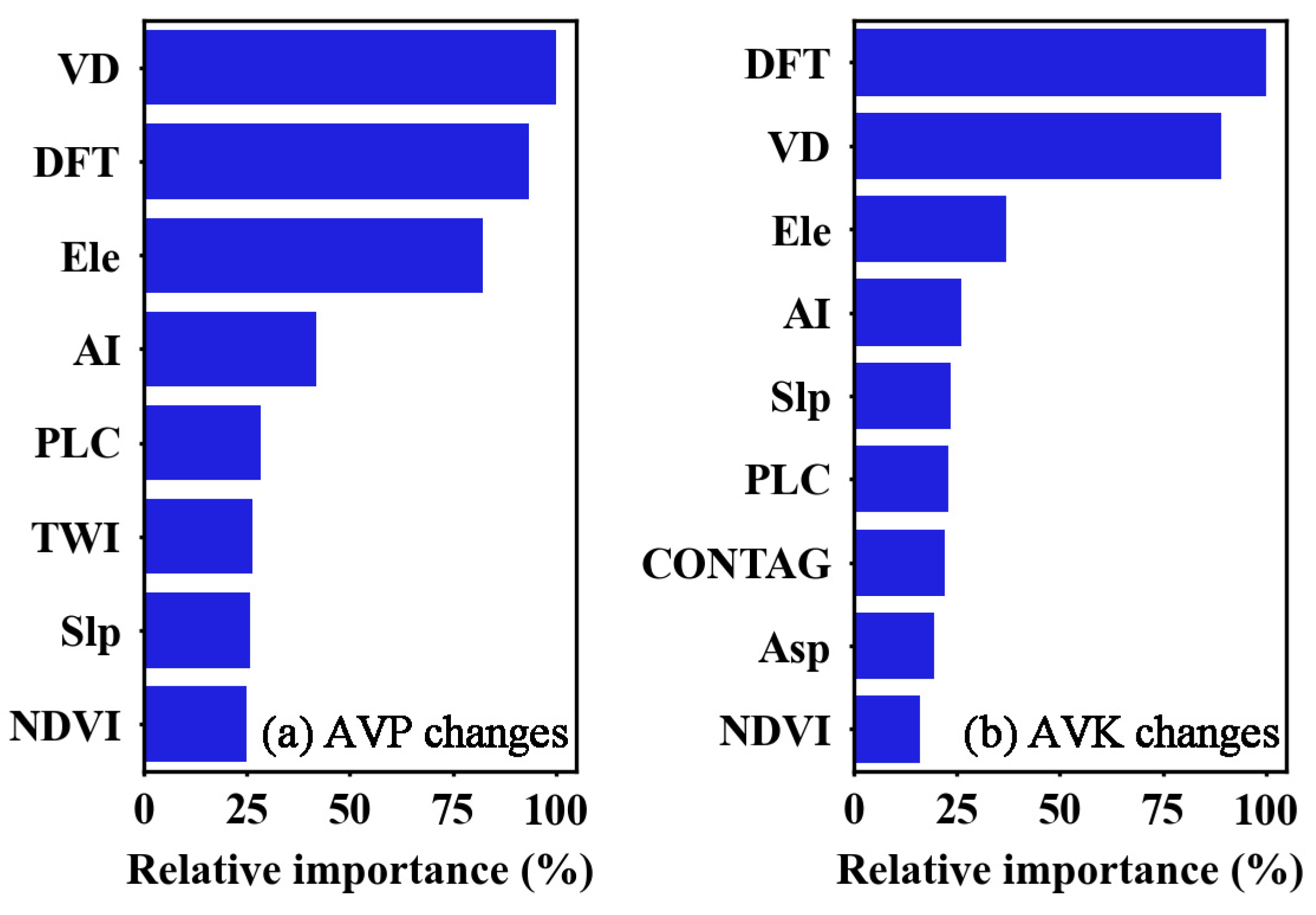
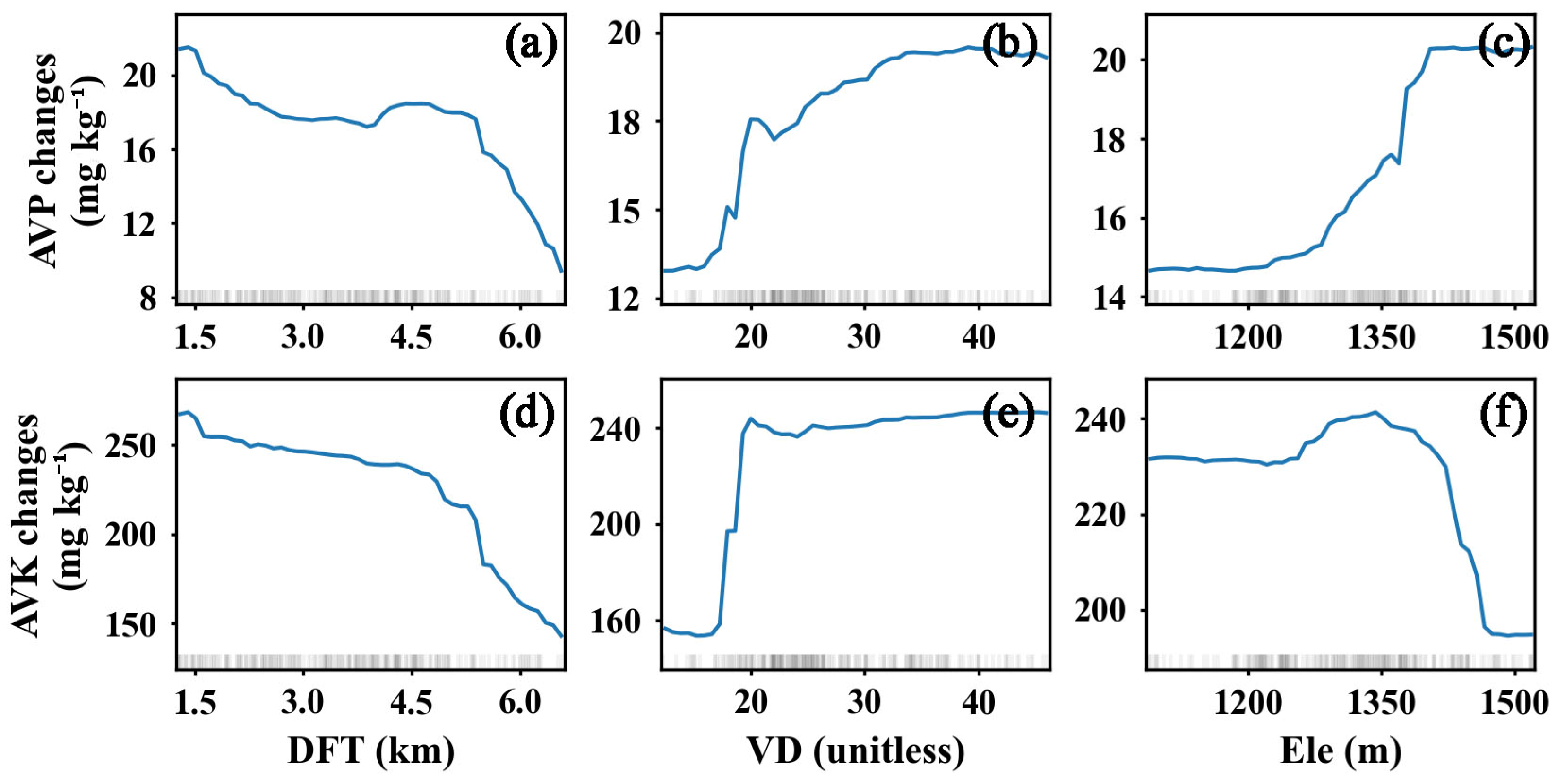
3.4. Relative Importance of Covariates and PDP Analysis

Model-E was iterated 100 times, and the mean relative importance of the environmental variables in predicting AVP and AVK changes was recorded and presented in Figure 5. DFT and VD were ranked as the top two most important variables, followed by elevation. The relative importance of the other variables was relatively low, and their contribution was generally around 25% of the most important variable.

3.5. Nonlinear Threshold and Interaction Effects of Key Factors

Given that the relative importance of DFT, VD, and Ele far outweighed those of other factors, their associations with AVP and AVK changes were visualized via PDP analysis (Figure 6). Generally, AVP and AVK changes were negatively related to DFT and positively correlated with VD. AVP changes increased along with elevation, while AVK changes showed a decreasing trend. All three variables exhibited non-linear threshold effects on AVP changes and AVK changes. Specifically, the effects of DFT and VD on AVP and AVK changes were mutated at 5 km and 20, respectively. These changes flattened when DFT < 5 km and VD > 20, decreased rapidly when DFT > 5 km, and increased drastically when VD ranged between 0 and 20. The AVP changes also increased dramatically when Ele ranged between 1298 m and 1390 m, while the AVK changes decreased rapidly when Ele ranged between 1350 m and 1466 m.
The bivariate interaction effects of the three most important environmental variables on AVP and AVK changes are visualized in Figure 7. Tobacco soils exhibited lower AVP and AVK accumulation in areas with VD < 20, and in areas with DFT > 5 km and VD ranging between 20 and 34. The effects of DFT and VD on AVP and AVK changes significantly varied across different elevations. Specifically, the relationship between DFT and AVP changes was roughly stable when Ele < 1298 m, while the effect of DFT on AVP changes exhibited a large abrupt change near DFT = 5 km in the area with Ele > 1390 m (Figure 7b). When Ele < 1466 m, the relationship between DFT and AVK changes fluctuated dramatically around DFT = 5 km, and when Ele > 1466 m, such a relationship was roughly stable (Figure 7e). In regions with Ele < 1390 m, the relationship between VD and AVP changes fluctuated dramatically when VD ranged between 20 and 33, but when Ele > 1390 m, such a relationship abruptly changed near VD = 20 (Figure 7c). At any altitude, the relationship between VD and AVK changes fluctuated at VD = 20, and this fluctuation was stronger at altitudes less than 1466 m (Figure 7f).

4. Discussion

4.1. Temporal Changes of AVP and AVK from 2012 to 2021

From 2012 to 2021, the AVP and AVK contents in tobacco fields increased significantly (p < 0.01) by 67.3% and 171.39%, respectively (Table 2), which were much higher than those in Chinese arable land. Specifically, the AVK content of China’s arable land increased by 15.1% between 1988–2007 and 2008–2018 [55]. Such a rapid increase in AVP and AVK content was inextricably linked to long-term heavy fertilization [27,28]. Given that tobacco is a high-value crop, farmers tend to apply higher amounts of chemical fertilizers in tobacco production than in staple crop production [27,28,55]. For example, the annual application of chemical K fertilizers for tobacco production is 2.16 to 2.52 times the average level used in Chinese farmland [55]. Moreover, the AVP and AVK contents in 2021 reached 48.25 mg kg−1 and 357.34 mg kg−1, respectively, which far exceeded the average values for Chinese farmland (27 mg kg−1 and 139 mg kg−1, respectively) [55,56]. Overall, the growth rates and current levels of AVP and AVK in tobacco fields were extremely high, which might pose numerous risks for tobacco production and the ecosystem, including low P/K use efficiency, resource wastage, and P leaching [11,12].

4.2. Effect of Socio-Geographical Factors on AVP Changes and AVK Changes

The addition of VD and DFT to the RF models greatly improved the prediction of AVP and AVK changes (Table 3). Moreover, VD and DFT obtained higher relative importance than the other factors in the optimal model (Figure 5). These findings underscore the importance of socio-geographical factors in controlling the variation in AVP and AVK changes. The socio-geographical factors can reflect potential human impacts on soil P and K [4,17,21,22,57]. Turner and Hiernaux [4] found that the distance to the nearest village exerts a greater influence on soil fertility parameters (e.g., soil P and K) than landscape position and soil physical properties. Similarly, Samaké et al. [17] revealed the close relationship of AVP and AVK contents with distance from villages in Sahel, Mali. The accumulation of P in soils in the European Union is closely related to the intensity of the livestock industry [57]. Road density and population density exert a greater direct influence on AVK content than topography and annual precipitation [21,22].
Humans always input P and K into agricultural soil through intentional actions (e.g., fertilizer application) and incidental behaviors (e.g., migration and deposition of chemical elements from enrichment sources controlled by precipitation and wind) [4]. In areas with larger VD and smaller DFT, such intentional actions are frequently observed, and the enrichment sources of P/K (e.g., rural livestock manure and domestic waste) are more abundant [4,17,21,22,58], thus explaining the negative and positive correlations of AVP and AVK changes with DFT (Figure 6a,d) and VD (Figure 6b,f), respectively. Similar findings have been reported in previous studies [4,17,21,22,59]. For example, Samaké et al. [17] revealed higher levels of soil P and K in fields located closer to villages and attributed this finding to unknown quantities of household waste and organic manure. Turner and Hiernaux [4] suggested that those fields located closer to villages are more likely to receive more agricultural inputs and net nutrient transfers from outlying areas. Chi et al. [60] reported a negative correlation between distance-related factors (e.g., distance from the mainland) and soil P/K, which might be due to the fact that in uninhabited islands, human impacts on soils are predominantly destructive instead of replenishing, unlike in intensively agricultural areas [4,17]. P and K elements from enrichment sources are also susceptible to transport and deposition to soils via precipitation and surface runoff [14], given that fields are typically located in sink areas, such as the foot of slopes or roadsides (Figure S1). Soils in areas located near town centers and in areas with high village density are also rich in black carbon, whose soil particle surface area is three times larger than that of normal soil, thereby reflecting its strong adsorption capacity to reduce the leaching loss of soil P and K [16,21].
In contrast to the linear response reported in previous studies [4,21,22], socio-geographical factors exerted nonlinear threshold effects on AVP and AVK changes in this study (Figure 6). The thresholds for the abrupt shift in the effect of DFT and VD on AVP and AVK changes were 5 km and 20, respectively. The AVP and AVK changes were flattened when DFT < 5 km and VD > 20, decreased rapidly when DFT > 5 km, and increased drastically when VD > 20. In other words, soil P and K accumulated more rapidly at locations near the town center (DFT < 5 km) and in areas with high village density (VD > 20). Fertilizer shops are mainly concentrated in towns. When tobacco fields are located too far from towns, the willingness of tobacco farmers to buy fertilizers may rapidly diminish due to the high transport costs and limited availability of transportation vehicles [58,61,62]. Tan et al. [62] found that manure from livestock farms is mainly exported to crop farms within a 5 km distance. Moreover, when the village density exceeds a certain threshold, the P and K from anthropogenic activities may exceed the loading capacity of the soil and thus lead to more drastic increases in AVP and AVK contents.

4.3. Influence of Other Environmental Variables

Elevation was ranked as the third most important topographic factor (Figure 5), whose influence on soil P and K variations has been well documented in the literature [1,2,3,34,35,36]. Elevation can control the (re)distribution of runoff and energy across landforms and therefore could explain the spatial variability in AVP and AVK changes [1,3]. Elevation positively affected AVP changes yet negatively controlled AVK changes (Figure 6). Previous studies have also reported the positive and negative effects of elevation on soil P (positively: He et al. [18]; negatively: Cheng et al. [35]; Nimalka Sanjeewani et al. [15]; Wang et al. [36]) and K (positively: Li et al. [1]; Nimalka Sanjeewani et al. [15]; negatively: Blanchet et al. [3]; Wang et al. [3]; Winzeler et al. [34]). The increase in soil K and P along with elevation is generally due to the enhanced weathering of bedrock [1,18] or decreased microbial activity [15]. The negative correlation of soil P and K with elevation is generally attributed to fine fractions (containing high P/K content) or surface-applied fertilizers, which are easily washed away to lower elevations by precipitation and surface runoff [34,36]. The final driving direction of elevation and soil P/K may depend on which force predominates in the study area. As the most popular topographic variable, elevation has been widely reported for its nonlinear threshold effects on soil properties [2,63], and similar observations were made in this study.
The index of landscape aggregation/connectivity (e.g., CONTAG and AI) was more important than the shape (e.g., LSI) and area factors (e.g., MPS) (Table S2). These findings are consistent with those of previous studies focusing on the Iranian plateau [33] and the northeastern plain of China [19], respectively. A connected landscape is conducive to the movement of materials across the region [25]. DFT and VD played a more important role in controlling the accumulation of soil P and K than topography and NDVI (Figure 5), thus supporting previous findings [4,21,22]. Moreover, AI contributed more than any other natural factor except for elevation (Figure 5). These results altogether show that the anthropogenic impacts on soil nutrients (e.g., P and K) in agricultural soils tend to be more profound than the impacts of natural factors [20,64,65].

4.4. Interaction Effects of the Three Most Important Environmental Variables

The relationship among DFT, VD, and AVP and AVK changes varied across different elevations (Figure 7). The interaction effects of natural (e.g., elevation) and other factors on soil P and K were confirmed in previous studies [1,20,22]. For example, topographic factors have significant effects on soil K, and these effects are enhanced by climate and soil properties [1]. Turner and Hiernaux [4] and Wang et al. [22] revealed the interaction effect of socio-geographical factors on soil P and K. The negative correlation between soil P and distance to villages diminishes when locational factors are controlled [4]. Population and road densities can affect AVK and K balance through complex interactions [22]. Despite the preliminary evidence showing the interaction of socio-economic factors on soil P and K, to our knowledge, the variation in these interactions across different environments has been rarely quantified. Apart from revealing the interaction effects of socio-geographical factors and elevation on AVP and AVK changes, this study is also the first to quantify the differences in these interactions across different altitudes (Figure 7). These interaction effects should be considered to understand the underlying processes leading to AVP and AVK changes in karst regions and to reveal the spatial variability in these changes.

4.5. Implications and Limitations

The tobacco soils across the study area generally have high P/K fertility levels and increased magnitude (Table 2). The AVP content in 2021 far exceeded the agronomic soil P threshold (17.3 mg kg−1) and slightly exceeded the environmental soil P threshold (40.1 mg kg−1) for Chinese soils [13,66]. Excessive soil P can severely inhibit the biological ability of crops to efficiently absorb and utilize P [66] and thus exacerbate the risk of non-point-source pollution [14]. Although excessive soil K does not imply an environmental problem, high surpluses of K may lead to an unbalanced composition of nutrients (e.g., low magnesium) in soils [3]. Overall, large surpluses of P and K in soils are harmful to tobacco production and the environment. Given that P and K resources are very limited in China [5], local agricultural departments should strengthen soil P and K management, especially in areas located near town centers (DFT < 5 km) and with high village density (VD > 20). According to the PDP analyses (Figure 6), soil P and K were highly susceptible to accumulation in these areas.
The Chinese government launched the third national soil census in 2022 [67], one important task of which was to accurately map soil properties. Improving the accuracy of digital mapping has been an important challenge in areas with complex terrain, such as karst [68,69]. Socio-geographical factors can improve the RF modeling accuracy for soil P and K (Table 3) and show a higher relative importance than the other factors (Figure 5). Therefore, socio-geographical factors can be useful indicators for improving the accuracy of soil property mapping.
This study focused on the effects of topography, socio-geographical factors, and landscape pattern indices on AVP and AVK changes in tobacco fields. The optimal model could explain 36% and 42% of the variance in AVP and AVK changes, respectively. The unexplained variations may be attributed to the following reasons: (1) soil erosion in mountainous areas can affect the accumulation of soil P and K [5], but high-precision soil erosion products are not accessible; and (2) similar to Minasny et al. [70], the spatial distribution of AVP and AVK in 2012 and 2021 was initially obtained by kriging interpolation, and then the spatial subtraction method was applied to calculate the temporal changes in AVP and AVK. However, kriging interpolation inevitably introduces uncertainty, thus influencing the modeling of AVP and AVK changes.

5. Conclusions

This study was conducted in a typical karstic mountainous agricultural region with a uniform geological type and low climatic variability. Results highlighted the temporal changes of AVP and AVK in tobacco fields, revealed the important influence of socio-geographical factors on these changes, and detected the nonlinear thresholds and interaction effects of these factors. The mean values of AVP (48.25 mg kg−1) and AVK in 2021 (357.67 mg kg−1) were significantly (p < 0.01) higher than those in 2012 (28.84 mg kg−1 and 131.67 mg kg−1, respectively). Based on the optimal RF model, the socio-geographical factors DFT and VD were identified as the two most important factors affecting AVP and AVK changes, followed by elevation. The results of the PDP analysis revealed that these three socio-geographical factors affected AVP and AVK changes in a nonlinear threshold pattern. AVP and AVK showed stronger accumulation from 2012 to 2021 at locations near the town center (DFT < 5 km) and in areas with high village density (VD > 20). AVP changes increased dramatically when Ele ranged between 1298 m and 1390 m, while AVK changes decreased rapidly when Ele ranged between 1350 m and 1466 m. The interaction effect of socio-geographical factors with elevation on AVP changes and AVK changes was determined, indicating that the relationship among DFT, VD, and AVP and AVK changes varied along with increasing elevation. These findings highlight the important role and complex patterns of socio-geographical factors in controlling the spatiotemporal variations in AVP and AVK. Therefore, these factors should be fully considered in mapping studies of soil P and K and when making agricultural decisions about controlling P and K surpluses in soils.

Supplementary Materials

The following supporting information can be downloaded at: https://www.mdpi.com/article/10.3390/land13060882/s1, Figure S1: Realistic map of tobacco fields from Google Earth Pro (109°26′02″, 30°41′0″) (Left) and field survey (Right). The red arrow represents the slope direction; Table S1: Semi-variogram parameters for soil available phosphorus (AVP) and soil available potassium (AVK) in 2012 and 2021. Table S2: Selected optimal variables for the RF model using the Boruta algorithm.

Author Contributions

Conceptualization, W.Z.; methodology, W.Z.; software, W.Z.; validation, W.W. and H.L.; formal analysis, W.Z., W.W. and H.L.; investigation, W.Z., X.Z. and Y.Z.; resources, Y.Z. and H.L.; data curation, Y.Z.; writing—original draft preparation, W.Z.; writing—review and editing, W.Z., W.W., X.Z. and Y.Z.; visualization, W.Z., X.Z. and Y.Z.; supervision, H.L.; project administration, H.L.; funding acquisition, H.L. All authors have read and agreed to the published version of the manuscript.

Funding

This research was funded by the Chongqing Key Laboratory of Digital Agriculture (China) and Chongqing Tobacco Science Research Institute (China).

Data Availability Statement

The original contributions presented in the study are included in the article/Supplementary Material, further inquiries can be directed to the corresponding author.

Acknowledgments

We thank the local farmers for their help during the sample collection.

Conflicts of Interest

Author Yunyi Zhang was employed by the company Chongqing Bureau of Geology and Minerals Exploration. The remaining authors declare that the research was conducted in the absence of any commercial or financial relationships that could be construed as a potential conflict of interest.

References

  1. Li, T.; Liang, J.; Chen, X.; Wang, H.; Zhang, S.; Pu, Y.; Xu, X.; Li, H.; Xu, J.; Wu, X.; et al. The Interacting Roles and Relative Importance of Climate, Topography, Soil Properties and Mineralogical Composition on Soil Potassium Variations at a National Scale in China. CATENA 2021, 196, 104875. [Google Scholar] [CrossRef]
  2. He, X.; Augusto, L.; Goll, D.S.; Ringeval, B.; Wang, Y.; Helfenstein, J.; Huang, Y.; Yu, K.; Wang, Z.; Yang, Y.; et al. Global Patterns and Drivers of Soil Total Phosphorus Concentration. Earth Syst. Sci. Data Discuss. 2021, 13, 5831–5846. [Google Scholar] [CrossRef]
  3. Blanchet, G.; Libohova, Z.; Joost, S.; Rossier, N.; Schneider, A.; Jeangros, B.; Sinaj, S. Spatial Variability of Potassium in Agricultural Soils of the Canton of Fribourg, Switzerland. Geoderma 2017, 290, 107–121. [Google Scholar] [CrossRef]
  4. Turner, M.D.; Hiernaux, P. The Effects of Management History and Landscape Position on Inter-Field Variation in Soil Fertility and Millet Yields in Southwestern Niger. Agric. Ecosyst. Environ. 2015, 211, 73–83. [Google Scholar] [CrossRef]
  5. Song, X.; Alewell, C.; Borrelli, P.; Panagos, P.; Huang, Y.; Wang, Y.; Wu, H.; Yang, F.; Yang, S.; Sui, Y. Pervasive Soil Phosphorus Losses in Terrestrial Ecosystems in China. Glob. Chang. Biol. 2024, 30, e17108. [Google Scholar]
  6. Ziadi, N.; Whalen, J.K.; Messiga, A.J.; Morel, C. Chapter Two—Assessment and Modeling of Soil Available Phosphorus in Sustainable Cropping Systems. Adv. Agron. 2013, 122, 85–126. [Google Scholar]
  7. Roger, A.; Libohova, Z.; Rossier, N.; Joost, S.; Maltas, A.; Frossard, E.; Sinaj, S. Spatial Variability of Soil Phosphorus in the Fribourg Canton, Switzerland. Geoderma 2014, 217–218, 26–36. [Google Scholar] [CrossRef]
  8. Liu, J.; Diamond, J. China’s Environment in a Globalizing World. Nature 2005, 435, 1179–1186. [Google Scholar] [CrossRef] [PubMed]
  9. MacDonald, G.K.; Bennett, E.M.; Potter, P.A.; Ramankutty, N. Agronomic Phosphorus Imbalances across the World’s Croplands. Proc. Natl. Acad. Sci. USA 2011, 108, 3086–3091. [Google Scholar] [CrossRef]
  10. Chen, W.; Geng, Y.; Hong, J.; Yang, D.; Ma, X. Life Cycle Assessment of Potash Fertilizer Production in China. Resour. Conserv. Recycl. 2018, 138, 238–245. [Google Scholar] [CrossRef]
  11. Steinfurth, K.; Hirte, J.; Morel, C.; Buczko, U. Conversion Equations between Olsen-P and Other Methods Used to Assess Plant Available Soil Phosphorus in Europe—A Review. Geoderma 2021, 401, 115339. [Google Scholar] [CrossRef]
  12. Chen, S.; Yan, Z.; Chen, Q. Estimating the Potential to Reduce Potassium Surplus in Intensive Vegetable Fields of China. Nutr. Cycl. Agroecosyst. 2017, 107, 265–277. [Google Scholar] [CrossRef]
  13. Zhang, W.; Chen, X.; Ma, L.; Deng, Y.; Cao, N.; Xiao, R.; Zhang, F.; Chen, X. Re-Prediction of Phosphate Fertilizer Demand in China Based on Agriculture Green Development. Acta Pedol. Sin. 2023, 60, 1389–1397, (In Chinese with English Abstract). [Google Scholar]
  14. Zhong, S.; Liu, W.; Ni, C.; Yang, Q.; Ni, J.; Wei, C. Runoff Harvesting Engineering and Its Effects on Soil Nitrogen and Phosphorus Conservation in the Sichuan Hilly Basin of China. Agric. Ecosyst. Environ. 2020, 301, 107022. [Google Scholar] [CrossRef]
  15. Nimalka Sanjeewani, H.K.; Samarasinghe, D.P.; De Costa, W.A.J.M. Influence of Elevation and the Associated Variation of Climate and Vegetation on Selected Soil Properties of Tropical Rainforests across a Wide Elevational Gradient. CATENA 2024, 237, 107823. [Google Scholar] [CrossRef]
  16. Glaser, B.; Lehmann, J.; Zech, W. Ameliorating Physical and Chemical Properties of Highly Weathered Soils in the Tropics with Charcoal—A Review. Biol. Fertil. Soils 2002, 35, 219–230. [Google Scholar] [CrossRef]
  17. Samaké, O.; Smaling, E.M.A.; Kropff, M.J.; Stomph, T.J.; Kodio, A. Effects of Cultivation Practices on Spatial Variation of Soil Fertility and Millet Yields in the Sahel of Mali. Agric. Ecosyst. Environ. 2005, 109, 335–345. [Google Scholar] [CrossRef]
  18. He, X.; Chu, C.; Yang, Y.; Shu, Z.; Li, B.; Hou, E. Bedrock and Climate Jointly Control the Phosphorus Status of Subtropical Forests along Two Elevational Gradients. CATENA 2021, 206, 105525. [Google Scholar] [CrossRef]
  19. Liu, X.; Li, S.; Wang, S.; Bian, Z.; Zhou, W.; Wang, C. Effects of Farmland Landscape Pattern on Spatial Distribution of Soil Organic Carbon in Lower Liaohe Plain of Northeastern China. Ecol. Indic. 2022, 145, 109652. [Google Scholar] [CrossRef]
  20. He, X.; Yang, L.; Li, A.; Zhang, L.; Shen, F.; Cai, Y.; Zhou, C. Soil Organic Carbon Prediction Using Phenological Parameters and Remote Sensing Variables Generated from Sentinel-2 Images. CATENA 2021, 205, 105442. [Google Scholar] [CrossRef]
  21. Liu, F.; Wang, X.; Chi, Q.; Tian, M. Spatial Variations in Soil Organic Carbon, Nitrogen, Phosphorus Contents and Controlling Factors across the “Three Rivers” Regions of Southwest China. Sci. Total Environ. 2021, 794, 148795. [Google Scholar] [CrossRef] [PubMed]
  22. Wang, S.; Li, Z.; Li, L.; Xu, Y.; Wu, G.; Liu, Q.; Peng, P.; Li, T. Soil Potassium Balance in the Hilly Region of Central Sichuan, China, Based on Crop Distribution. Sustainability 2023, 15, 15348. [Google Scholar] [CrossRef]
  23. Wadoux, A.M.-C.; Molnar, C. Beyond Prediction: Methods for Interpreting Complex Models of Soil Variation. Geoderma 2022, 422, 115953. [Google Scholar] [CrossRef]
  24. Petermann, E.; Meyer, H.; Nussbaum, M.; Bossew, P. Mapping the Geogenic Radon Potential for Germany by Machine Learning. Sci. Total Environ. 2021, 754, 142291. [Google Scholar] [CrossRef] [PubMed]
  25. Wu, Z.; Chen, Y.; Yang, Z.; Liu, Y.; Zhu, Y.; Tong, Z.; An, R. Spatial Distribution of Lead Concentration in Peri-Urban Soil: Threshold and Interaction Effects of Environmental Variables. Geoderma 2023, 429, 116193. [Google Scholar] [CrossRef]
  26. Wang, K.; Zhang, C.; Chen, H.; Yue, Y.; Zhang, W.; Zhang, M.; Qi, X.; Fu, Z. Karst Landscapes of China: Patterns, Ecosystem Processes and Services. Landsc. Ecol. 2019, 34, 2743–2763. [Google Scholar] [CrossRef]
  27. Liu, G.; Deng, L.; Wu, R.; Guo, S.; Du, W.; Yang, M.; Bian, J.; Liu, Y.; Li, B.; Chen, F. Determination of Nitrogen and Phosphorus Fertilisation Rates for Tobacco Based on Economic Response and Nutrient Concentrations in Local Stream Water. Agric. Ecosyst. Environ. 2020, 304, 107136. [Google Scholar] [CrossRef]
  28. Zhang, W.-C.; Wu, W.; Liu, H.-B. Planting Year-and Climate-Controlled Soil Aggregate Stability and Soil Fertility in the Karst Region of Southwest China. Agronomy 2023, 13, 2962. [Google Scholar] [CrossRef]
  29. Chen, S.; Arrouays, D.; Leatitia Mulder, V.; Poggio, L.; Minasny, B.; Roudier, P.; Libohova, Z.; Lagacherie, P.; Shi, Z.; Hannam, J.; et al. Digital Mapping of GlobalSoilMap Soil Properties at a Broad Scale: A Review. Geoderma 2022, 409, 115567. [Google Scholar] [CrossRef]
  30. Institute of Soil Science, Chinese Academy Science (ISSCAS). Soil Physical and Chemical Analysis; Shanghai Science and Technology Press: Shanghai, China, 1978. (In Chinese) [Google Scholar]
  31. McBratney, A.B.; Mendonça Santos, M.L.; Minasny, B. On Digital Soil Mapping. Geoderma 2003, 117, 3–52. [Google Scholar] [CrossRef]
  32. Jenny, H. Factors of Soil Formation: A System of Quantitative Pedology; Courier Corporation: North Chelmsford, MA, USA, 1994; ISBN 0486681289. [Google Scholar]
  33. Ahmadi Mirghaed, F.; Souri, B. Spatial Analysis of Soil Quality through Landscape Patterns in the Shoor River Basin, Southwestern Iran. CATENA 2022, 211, 106028. [Google Scholar] [CrossRef]
  34. Winzeler, H.E.; Owens, P.R.; Joern, B.C.; Camberato, J.J.; Lee, B.D.; Anderson, D.E.; Smith, D.R. Potassium Fertility and Terrain Attributes in a Fragiudalf Drainage Catena. Soil Sci. Soc. Am. J. 2008, 72, 1311–1320. [Google Scholar] [CrossRef]
  35. Cheng, Y.; Li, P.; Xu, G.; Li, Z.; Cheng, S.; Gao, H. Spatial Distribution of Soil Total Phosphorus in Yingwugou Watershed of the Dan River, China. CATENA 2016, 136, 175–181. [Google Scholar] [CrossRef]
  36. Wang, H.J.; Shi, X.Z.; Yu, D.S.; Weindorf, D.C.; Huang, B.; Sun, W.X.; Ritsema, C.J.; Milne, E. Factors Determining Soil Nutrient Distribution in a Small-Scaled Watershed in the Purple Soil Region of Sichuan Province, China. Soil Tillage Res. 2009, 105, 300–306. [Google Scholar] [CrossRef]
  37. Gorelick, N.; Hancher, M.; Dixon, M.; Ilyushchenko, S.; Thau, D.; Moore, R. Google Earth Engine: Planetary-Scale Geospatial Analysis for Everyone. Remote Sens. Environ. 2017, 202, 18–27. [Google Scholar] [CrossRef]
  38. NASA; METI. AIST, Japan Spacesystems and US/Japan ASTER Science Team: ASTER Global Digital Elevation Model V003, NASA EOSDIS Land Processes DAAC [Data Set] 2019. Available online: https://lpdaac.usgs.gov/products/astgtmv003/ (accessed on 22 January 2022).
  39. McGarigal, K.; Cushman, S.A.; Neel, M.C.; Ene, E. Spatial Pattern Analysis Program for Categorical Maps. 2002. Available online: https://fragstats.org/ (accessed on 28 January 2024).
  40. ESRI. ArcGIS Desktop, Release 10; Environmental Systems Research Institute: Redlands, CA, USA, 2011; Available online: https://www.scirp.org/reference/ReferencesPapers?ReferenceID=1102852 (accessed on 10 June 2024).
  41. IBM Corp. IBM SPSS Statistics for Windows; Version 22.0; IBM Corp: Armonk, NY, USA, 2013. [Google Scholar]
  42. Cambardella, C.A.; Moorman, T.B.; Novak, J.M.; Parkin, T.B.; Karlen, D.L.; Turco, R.F.; Konopka, A.E. Field-Scale Variability of Soil Properties in Central Iowa Soils. Soil Sci. Soc. Am. J. 1994, 58, 1501–1511. [Google Scholar] [CrossRef]
  43. Lu, L.; Li, S.; Gao, Y.; Ge, Y.; Zhang, Y. Analysis of the Characteristics and Cause Analysis of Soil Salt Space Based on the Basin Scale. Appl. Sci. 2022, 12, 9022. [Google Scholar] [CrossRef]
  44. Anselin, L. Local Indicators of Spatial Association—LISA. Geogr. Anal. 1995, 27, 93–115. [Google Scholar] [CrossRef]
  45. Breiman, L. Random Forests. Mach. Learn. 2001, 45, 5–32. [Google Scholar] [CrossRef]
  46. Zhang, X.; Chen, S.; Xue, J.; Wang, N.; Xiao, Y.; Chen, Q.; Hong, Y.; Zhou, Y.; Teng, H.; Hu, B.; et al. Improving Model Parsimony and Accuracy by Modified Greedy Feature Selection in Digital Soil Mapping. Geoderma 2023, 432, 116383. [Google Scholar] [CrossRef]
  47. Kursa, M.B.; Rudnicki, W.R. Feature Selection with the Boruta Package. J. Stat. Softw. 2010, 36, 1–13. [Google Scholar] [CrossRef]
  48. Friedman, J.H. Greedy Function Approximation: A Gradient Boosting Machine. Ann. Stat. 2001, 29, 1189–1232. [Google Scholar] [CrossRef]
  49. Molnar, C. Interpretable Machine Learning; Lulu.com: Morrisville, NC, USA, 2020; ISBN 0244768528. [Google Scholar]
  50. Wilding, L.P. Spatial Variability: Its Documentation, Accomodation and Implication to Soil Surveys. In Proceedings of the Soil Spatial Variability, Las Vegas, NV, USA, 30 November–1 December 1984; pp. 166–194. [Google Scholar]
  51. Bedeian, A.G.; Mossholder, K.W. On the Use of the Coefficient of Variation as a Measure of Diversity. Organ. Res. Methods 2000, 3, 285–297. [Google Scholar] [CrossRef]
  52. Duan, L.; Li, Z.; Xie, H.; Yuan, H.; Li, Z.; Zhou, Q. Regional Pattern of Soil Organic Carbon Density and Its Influence upon the Plough Layers of Cropland. Land Degrad. Dev. 2020, 31, 2461–2474. [Google Scholar] [CrossRef]
  53. Kravchenko, A.N. Influence of Spatial Structure on Accuracy of Interpolation Methods. Soil Sci. Soc. Am. J. 2003, 67, 1564–1571. [Google Scholar] [CrossRef]
  54. Garten, C.T.; Kang, S.; Brice, D.J.; Schadt, C.W.; Zhou, J. Variability in Soil Properties at Different Spatial Scales (1m–1km) in a Deciduous Forest Ecosystem. Soil Biol. Biochem. 2007, 39, 2621–2627. [Google Scholar] [CrossRef]
  55. Liu, K.; Du, J.; Ma, C.; Qu, X.; Han, T.; Liu, S.; Huang, J.; Li, Y.; Shen, Z.; Zhang, L. Spatio-Temporal Evolution Characteristics of Soil Potassium in Main Dry-Farming Grain Arable Land of China. ACTA Pedol. Sin. 2022, 60, 673–684, (In Chinese with English Abstract). [Google Scholar]
  56. Zhan, X.; Ren, Y.; Zhang, S.; Kang, R. Changes in Olsen Phosphorus Concentration and Its Response to Phosphorus Balance in the Main Types of Soil in China. Sci. Agric. Sin. 2015, 48, 4728–4737, (In Chinese with English Abstract). [Google Scholar]
  57. Tóth, G.; Guicharnaud, R.-A.; Tóth, B.; Hermann, T. Phosphorus Levels in Croplands of the European Union with Implications for P Fertilizer Use. Eur. J. Agron. 2014, 55, 42–52. [Google Scholar] [CrossRef]
  58. Mukai, S. Combined Agronomic and Economic Modeling in Farmers’ Determinants of Soil Fertility Management Practices: Case Study from the Semi-Arid Ethiopian Rift Valley. Agriculture 2023, 13, 281. [Google Scholar] [CrossRef]
  59. Liu, R.; Xu, F.; Yu, W.; Shi, J.; Zhang, P.; Shen, Z. Analysis of Field-Scale Spatial Correlations and Variations of Soil Nutrients Using Geostatistics. Environ. Monit. Assess. 2016, 188, 126. [Google Scholar] [CrossRef] [PubMed]
  60. Chi, Y.; Sun, J.; Fu, Z.; Xie, Z. Which Factor Determines the Spatial Variance of Soil Fertility on Uninhabited Islands? Geoderma 2020, 374, 114445. [Google Scholar] [CrossRef]
  61. Chadwick, D.; Jia, W.; Tong, Y.; Yu, G.; Shen, Q.; Chen, Q. Improving Manure Nutrient Management towards Sustainable Agricultural Intensification in China. Agric. Ecosyst. Environ. 2015, 209, 34–46. [Google Scholar] [CrossRef]
  62. Tan, M.; Hou, Y.; Zhang, T.; Ma, Y.; Long, W.; Gao, C.; Liu, P.; Fang, Q.; Dai, G.; Shi, S.; et al. Relationships between Livestock Density and Soil Phosphorus Contents—County and Farm Level Analyses. CATENA 2023, 222, 106817. [Google Scholar] [CrossRef]
  63. Guo, P.T.; Li, M.F.; Luo, W.; Tang, Q.F.; Liu, Z.W.; Lin, Z.M. Digital Mapping of Soil Organic Matter for Rubber Plantation at Regional Scale: An Application of Random Forest plus Residuals Kriging Approach. Geoderma 2015, 237–238, 49–59. [Google Scholar] [CrossRef]
  64. Demay, J.; Ringeval, B.; Pellerin, S.; Nesme, T. Half of Global Agricultural Soil Phosphorus Fertility Derived from Anthropogenic Sources. Nat. Geosci. 2023, 16, 69–74. [Google Scholar] [CrossRef]
  65. Guo, J.H.; Liu, X.J.; Zhang, Y.; Shen, J.L.; Han, W.X.; Zhang, W.F.; Christie, P.; Goulding, K.W.T.; Vitousek, P.M.; Zhang, F.S. Significant Acidification in Major Chinese Croplands. Science 2010, 327, 1008–1010. [Google Scholar] [CrossRef]
  66. Wang, Y.; Cui, Y.; Wang, K.; He, X.; Dong, Y.; Li, S.; Wang, Y.; Yang, H.; Chen, X.; Zhang, W. The Agronomic and Environmental Assessment of Soil Phosphorus Levels for Crop Production: A Meta-Analysis. Agron. Sustain. Dev. 2023, 43, 35. [Google Scholar] [CrossRef]
  67. National Council. Notice from the State Council of Launching the Third National Soil Survey. 2022. Available online: https://english.www.gov.cn/policies/latestreleases/202202/16/content_WS620caf99c6d09c94e48a51cb.html (accessed on 22 January 2022).
  68. Zhang, W.; Wan, H.; Zhou, M.; Wu, W.; Liu, H. Soil Total and Organic Carbon Mapping and Uncertainty Analysis Using Machine Learning Techniques. Ecol. Indic. 2022, 143, 109420. [Google Scholar] [CrossRef]
  69. Wadoux, A.M.J.C.; Heuvelink, G.B.M.; Lark, R.M.; Lagacherie, P.; Bouma, J.; Mulder, V.L.; Libohova, Z.; Yang, L.; McBratney, A.B. Ten Challenges for the Future of Pedometrics. Geoderma 2021, 401, 115155. [Google Scholar] [CrossRef]
  70. Minasny, B.; Hong, S.Y.; Hartemink, A.E.; Kim, Y.H.; Kang, S.S. Soil PH Increase under Paddy in South Korea between 2000 and 2012. Agric. Ecosyst. Environ. 2016, 221, 205–213. [Google Scholar] [CrossRef]
Figure 1. Digital elevation model, location of the study area, and sampling points in 2012 (N = 138) and 2021 (N = 117).
Land 13 00882 g001
Figure 2. Spatial distribution maps of 13 environmental variables.
Land 13 00882 g002
Figure 3. Semi-variogram plots of soil available phosphorus (AVP) and soil available potassium (AVK) in 2012 and 2021. Co: nugget variance; Co + C: sill variance; Co/(Co + C): nugget effect.
Land 13 00882 g003
Figure 4. Spatial distribution maps for AVP in 2012 (a), AVP in 2021 (b), AVP changes and LISA cluster (c), AVK in 2012 (d), AVK in 2021 (e), and AVP changes and LISA cluster (f). AVP: soil available phosphorus; AVK: soil available potassium; high–high: high value in a high-value neighborhood; low–low: low value in a low-value neighborhood.
Land 13 00882 g004
Figure 5. The relative importance of independent variables for AVP changes (a) and AVK changes (b). Note: AVP: soil available phosphorus; AVK: soil available potassium; NDVI: normalized difference vegetation index; Ele: elevation; Slp: slope; Asp: aspect; PLC: plane curvature; TWI: topographical wetness index; AI: aggregation index; CONTAG: landscape contagion index; DFT: distance from the nearest town center; VD: village density.
Land 13 00882 g005
Figure 6. Partial dependence plots of the top three environmental variables for AVP changes (ac) and AVK changes (df). The black bands along the x-axis visualize the distribution of data. Note: AVP: soil available phosphorus; AVK: soil available potassium; DFT: distance from the nearest town center; VD: village density; Ele: elevation.
Land 13 00882 g006
Figure 7. Two-way interaction effects of the three most important environmental variables for AVP changes (ac) and AVK changes (df). Note: DFT: distance from the nearest town center; VD: village density; Ele: elevation.
Land 13 00882 g007
Table 1. Environmental variables used in this study.
TypeVariablesAbbreviationUnitData Source
BiologyNormalized difference vegetation indexNDVIunitlessGoogle Earth Engine platform
TopographyElevationElemASTER GDEM v3
SlopeSlp°
AspectAsp°
Plane curvaturePLCrad m−1
Profile curvaturePRCrad m−1
Topographical wetness indexTWIunitless
Landscape
pattern
Patch sizeMPShaLand use map, Chongqing Provincial Department of Land and Resources
Landscape contagion indexCONTAG%
Aggregation indexAI%
Landscape shape indexLSIunitless
Socio-geographical
factors
Village densityVDunitlessLand use map and Google Earth Pro platform
Distance from the nearest town centerDFTkm
Table 2. Descriptive statistics for soil available phosphorus (AVP), soil available potassium (AVK), and environmental variables.
ItemAbbreviationUnitMinimumMaximumMedianMeanSDCV (%)Skewness
AVP in 2012AVP2012mg kg−10.68110.1523.6128.8421.1173.181.28
AVP in 2021AVP2021mg kg−14.70130.4045.1548.2524.7651.320.79
AVK in 2012AVK2012mg kg−132.12371.44117.5131.6770.4653.511.12
AVK in 2021AVK2021mg kg−197.54782.79332.01357.34155.2643.450.68
Normalized difference vegetation indexNDVIunitless0.350.800.660.650.0710.74−0.79
ElevationElem1000166713241314.11134.0610.20−0.18
SlopeSlp°0.0051.284.757.559.72128.781.87
AspectAsp°0.01360145.49169.92107.6163.330.25
Plane curvaturePLCrad m−1−7 × 10−35.1 × 10−3−9 × 10⁻⁷−2 × 10−41.7 × 10−3/−0.76
Profile curvaturePRCrad m−1−1.17 × 10−24.7 × 10−3−1.17 × 10⁻³−1.4 × 10−32.2 × 10−3/−0.99
Topographical wetness indexTWIunitless3.6521.979.5710.204.4143.200.66
Aggregation indexAI%70.4110081.7881.814.094.99−0.23
Landscape contagion indexCONTAG%0.0057.6125.3025.329.4537.330.56
Landscape shape indexLSIunitless1.002.491.701.730.2212.480.86
Patch sizeMPSha3.1575.695.826.654.8272.531.36
Distance the from nearest town centerDFTkm0.657.774.973.651.5943.50.32
Village densityVDunitless4.58228.7525.3929.4421.3872.616.77
Note: /: PLC and PRC have both positive and negative values, which typically means that the CVs are meaningless [51]. All sample points in 2012 (N = 138) and 2021 (N = 117) were used for the descriptive statistics.
Table 3. Performance of all five models for AVP changes and AVK changes using random forest models based on 100 repetitions (mean ± standard deviation).
ItemMetricsModel-AModel-BModel-CModel-DModel-E
AVP changesR20.14 ± 0.140.17 ± 0.130.33 ± 0.160.36 ± 0.130.41 ± 0.14
(mg kg−1)RMSE8.50 ± 0.778.39 ± 0.757.51 ± 0.867.34 ± 0.777.11 ± 0.79
AVK changesR20.15 ± 0.120.16 ± 0.100.42 ± 0.120.40 ± 0.110.44 ± 0.13
(mg kg−1)RMSE71.21 ± 6.5769.88 ± 6.6458.01 ± 6.4858.91 ± 6.6956.89 ± 6.57
Note: Model-A: NDVI and topographic variables; Model-B: NDVI, topographic variables and landscape pattern; Model-C: NDVI, topographic variables and socio-geographical factors; Model-D: included all variables; Model-E: optimal variables obtained by the Boruta algorithm. AVP: soil available phosphorus; AVK: soil available potassium.
Disclaimer/Publisher’s Note: The statements, opinions and data contained in all publications are solely those of the individual author(s) and contributor(s) and not of MDPI and/or the editor(s). MDPI and/or the editor(s) disclaim responsibility for any injury to people or property resulting from any ideas, methods, instructions or products referred to in the content.

