Optimizing Territorial Spatial Structures within the Framework of Carbon Neutrality: A Case Study of Wuan

Abstract

Climate change has become a major worldwide problem, and land use/cover change has consistently played a crucial role in impacting the carbon cycle within terrestrial ecosystems. Territorial spatial planning stands as a relatively good policy option for the low-carbon model. The spatial correlation between carbon emissions and land use was established through environmental parameters in this paper. The territorial spatial structures in 2035 and 2060 under two scenarios of natural evolution and low-carbon development were simulated through the PLUS model. The results indicate that the spatial pattern of decreasing carbon emissions centered on towns, cities, mines, and industries is related to regional economic development, the distribution of forests, and the urban ecological environment. The implementation of territorial spatial planning aids in achieving carbon neutrality, whereas the low-carbon development scenario is more focused on it, which can provide ideas for territorial spatial planning adjustments. Both scenarios result in a large area of fallow land, indicating some conflict between farmland protection and low-carbon development. Optimizing management measures, energy structure, and industrial layout and strengthening regional coordination are key to promoting low-carbon development. This study might be useful in formulating regional carbon-neutral policies and improving territorial spatial planning.

1. Introduction

Recently, human society has developed rapidly because of advancements in science and technology and the increasing global economic status. Concurrently, the severity of global warming has increased [1]. Relevant studies have shown a rise in atmospheric CO₂ levels of more than a quarter because of human activities [2]. Since 2007, China has been responsible for 27% of the world’s carbon emissions, a statistic leading to China surpassing other countries as the top global carbon emitter [3]. To achieve sustainable development, China has concentrated its efforts on addressing climate change, insisting on low-carbon economic development. In 2007, China issued the China National Climate Change Programme. Since then, China has entered the nascent stage of a low-carbon economic strategy. Since the 11th Five-Year Plan period, China has successively constructed three constraints, namely, the level of energy consumption per unit of GDP, carbon dioxide emissions per unit of GDP, and the proportion of non-fossil energy in primary energy consumption. After 2011, China officially entered the deepening phase of its low-carbon economic strategy. China’s low-carbon policy has long been committed to saving energy and reducing pollutant emissions. Initially, it emphasized both pollution prevention and ecological protection. In the nascent stage of low-carbon economic strategy, it focused on energy conservation and emission reduction. Finally, it has gradually evolved into a low-carbon policy system of “synergizing energy conservation, pollution reduction and carbon emission reduction” in the deepening phase of the policy. In 2015, China participated in the United Nations Climate Conference in Paris and submitted the Enhanced Action on Climate Change—The Intended Nationally Determined Contributions, which sets control targets for carbon dioxide, energy use, and the number of forests to be controlled by 2030. The introduction of the carbon peaking and carbon neutrality goals means that China has placed its low-carbon strategy at an unprecedented level [4].

The concept of land use/cover change is crucial in driving climate change both regionally and globally, as it facilitates the exchange of energy and materials on terrestrial surfaces [5]. Researchers indicate that changes in land use contribute to approximately 30% of the world’s total human-made carbon emissions [6,7,8]. Land-use transfer has always been the primary determinant of the carbon cycle in terrestrial ecosystems [9], second only to energy combustion. Land-use carbon emissions studies provide an integrated perspective for understanding the carbon cycle in social-ecological systems. These studies include studies on land-use carbon emission effects [10,11], accounting methods [12,13,14], and land-use optimization [15,16,17].

Over the years, a great deal of research has been conducted on quantifying carbon emissions from land use. Land-use carbon emissions are affected by a combination of natural ecological processes and human economic activities and have different estimation methods. Among the carbon emission factor standards worldwide, the IPCC Guidelines for National Greenhouse Gas Inventories are the most influential [18], providing an overall reference for carbon emission accounting research. However, when analyzed at the regional level, these guidelines cannot reflect regional differences, complexity, and uniqueness. The inventory reflects the average level at the national level. China is a vast country with an uneven distribution of land types and a very uneven level of economic development, so the level of carbon emissions varies greatly from region to region. The results of regional carbon emissions using the inventory to calculate are inaccurate. Therefore, some scholars may focus on other methods to account for regional carbon emissions, which include the model estimation method represented by the bookkeeping model [19], the plot method [20], the actual measurement method, and the material balance method [21]. However, the above methods have problems such as high cost, operation difficulty, and low precision. The data of the model estimation method are mostly qualitative information, and the estimation accuracy is not high. The plot method has precise data and accurate calculation results, but it requires more instruments and multi-point deployment, so the observation cost is higher. The actual measurement method has a rigorous calculation process and high accuracy but long single continuous observation time, which leads to its relatively high cost and narrow application scope. The cost consumption of the material balance method is low, but the intermediate process is more, which makes it easy to cause errors. The carbon emission factor method is still dominant in practical applications. How to improve the accuracy of the coefficients so that they can accurately reflect the differences between regions has emerged as a critical issue requiring resolution.

In the context of global climate change, accurate spatial distribution calculations of carbon emissions/absorption are essential for future sustainable development. Efforts have been made to spatialize carbon emissions [22,23,24,25]. In particular, space information technology has provided new methods for monitoring surface data and obtaining spatialization results for carbon emissions [26]. Under the premise of limited carbon emission data, it is combined with remote sensing data for macro estimation, which is called the remote sensing map estimation method. The remote sensing data used include NPP [27,28], Landsat TM [29], NOAA/AVHRR [30], VIIRS-NPP [31], and so on. By employing remote sensing data and products, it is possible to acquire and link variables such as the normalized vegetation index (NDVI) and land surface temperature (LST) with carbon emissions across various land use types. Consequently, merging environmental factors linked to land utilization to gather data on the spatial diversity of carbon emissions represents a valuable strategy.

Land use scenario simulation is an important method for optimizing territorial space, and the core idea is optimizing the land use structure and simulating future spatial patterns. The number of sites in different areas is predicted and restructured according to certain development goals, and the future pattern is optimally modeled according to the current suitability of the spatial units within the constraints of this predicted number. Spatial simulation, which can promote the implementation of the carbon peaking and carbon neutrality goals at the regional level, is highly practical in building a spatial pattern of national territory with low carbon emissions. Territorial spatial planning, on the other hand, provides a realistic opportunity to carry out low-carbon optimization of land use and provides a path for humans to mitigate and adapt to global warming. Land use and land cover (LULC) simulation models serve as potent instruments for examining the origins and impacts of upcoming landscape changes in various situations [32]. Commonly used forecasting models for structural quantity include Markov [33], system dynamics (SD) [34], and multi-objective planning (MOP) [35] models. In terms of spatial pattern prediction, rooted in the conventional model of cellular automata (CA) [36], scholars have developed CLUE-S [37], FLUS [3,38], SLEUTH [39], and other models to simulate the spatial pattern of the national territory. Patch-generating Land Use Simulation (PLUS) is a CA model that amalgamates a strategy for analyzing land expansion with a seed-generation mechanism on the basis of multiple types of stochastic patches. In contrast to alternative models, the PLUS model boasts greater simulation precision and landscape designs more akin to actual landscapes [40] and is extensively utilized across various levels, including regional [41], national [42], provincial [43], and municipal [44,45] scales. However, it has not been validated in small-scale regions, such as counties. There is a lack of consideration of policy orientation and integrated perspectives in practical applications. Failure to consider policy orientation will make the simulation results rely mainly on historical change trends, ignoring the new requirements for land use types in the new stage of social development. The results of simulations oriented to a single goal only and lacking an integrated perspective do not take into account the needs of integrated social development and are not practically informative.

In this study, Wuan was selected as the study area. The spatial data of land use from 2012 to 2022 were used to account for the carbon emissions from land use within a decade, and the spatial heterogeneity was obtained by combining the environmental factors. The territorial spatial patterns under two scenarios of natural evolution and low-carbon development in 2035 and 2060 were simulated. The future land use carbon emissions under different scenarios with projected results and targets of territorial spatial planning were calculated. The role of territorial spatial planning and low-carbon development policies in contributing to carbon neutrality was explored. On a national or global scale, the environmental parameters introduced in this study provide a new method for estimating the spatial distribution of carbon emissions. This study accounts for multiple factors of territorial spatial planning, economy, ecology, and carbon emissions, which addresses the lack of research in this field. It provides a more comprehensive optimization method for low-carbon land use patterns on a national or global scale. This study provides a reference for carrying out territorial spatial optimization and achieving carbon emission reduction, as well as carbon peaking and carbon neutrality goals.

2. Materials and Methods

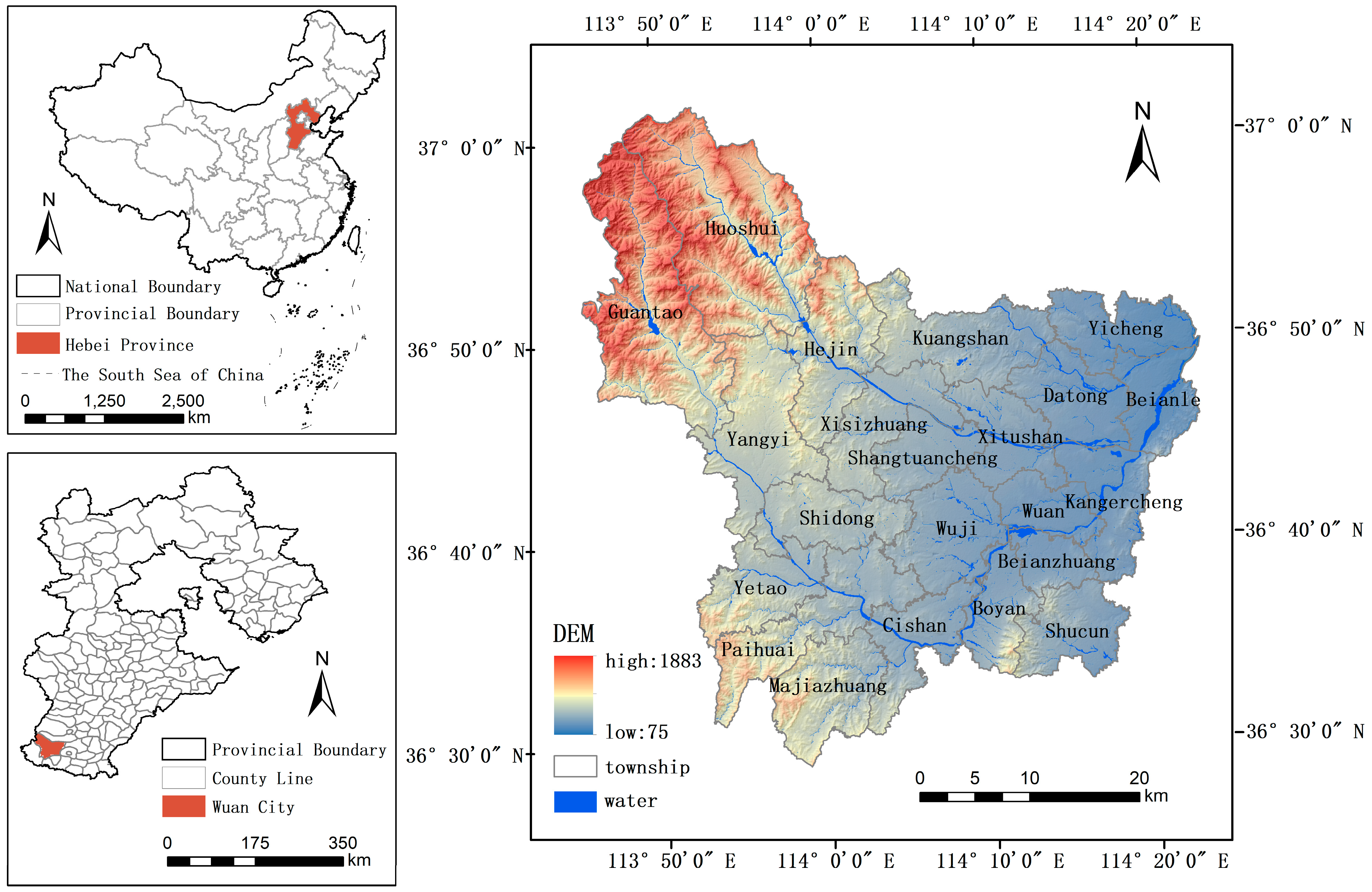
2.1. Study Area

Wuan is subordinate to Handan in Hebei Province. It spans latitudes 36°28′ to 37°01′ N and longitudes 113°45′ to 114°22′ E (Figure 1) and covers a total area of 1818.05 km². Wuan is one of the 58 key coal-producing counties and one of the four major iron-rich ore bases in China. Wuan is rich in mineral resources but has a low degree of comprehensive utilization. The ecological environment has been severely damaged as a result of the long-term neglect of ecological environmental protection and the rehabilitation of mines in the process of mineral resource development. As urbanization has rapidly progressed, the large demand for land resources has intensified the evolution of land use change in this region. Farmlands and grasslands have been infringed upon to varying degrees. The ecological space has been compressed, which affects the ecological environment and reduces the effect of carbon sinks.

2.2. Data Resources

In this paper, the data include statistical, planning, land use, driving data, and environmental parameters (

Table 1. Data resources.

Type	Name		Data Sources and Processing
Statistical data	Energy consumption by sector, volume of agricultural production activities, food production, effective irrigated area, total agricultural output, etc.		Wuan Statistical Yearbook (2012–2022)
Planning data	Planning information such as the protective index of farmland, ecological spatial constraints, and the planning targets for each category of area in 2035		Wuan Territorial Spatial Planning (2021–2035)
Land use data	Land-use change survey data, 2012–2022		The original vector data were converted to raster data in ArcGIS 10.8and were reclassified into six types of land use.
Environmental parameters	LST		Geographic remote sensing ecological network platform
	NDVI		MODIS dataset from USGS
Driving data	Physical geography	elevation, slope, aspect	The original DEM data obtained from the GDCP were processed in ArcGIS 10.8 to obtain the slope and aspect.
	Transport accessibility	distance to major roads, motorways, railways	Data on the road network were sourced from OSM and processed in ArcGIS 10.8 using the Euclidean distance tool to obtain transport accessibility.
	Socioeconomic	GDP, population density	GDP data were from the Resource and Environment Science and Data Centre. Population density data from the World POP were processed in ArcGIS 10.8.
	POI data	Density of points of interest	POI data were from the OSM and processed using the Kernel Density Analysis tool in ArcGIS 10.8.

).

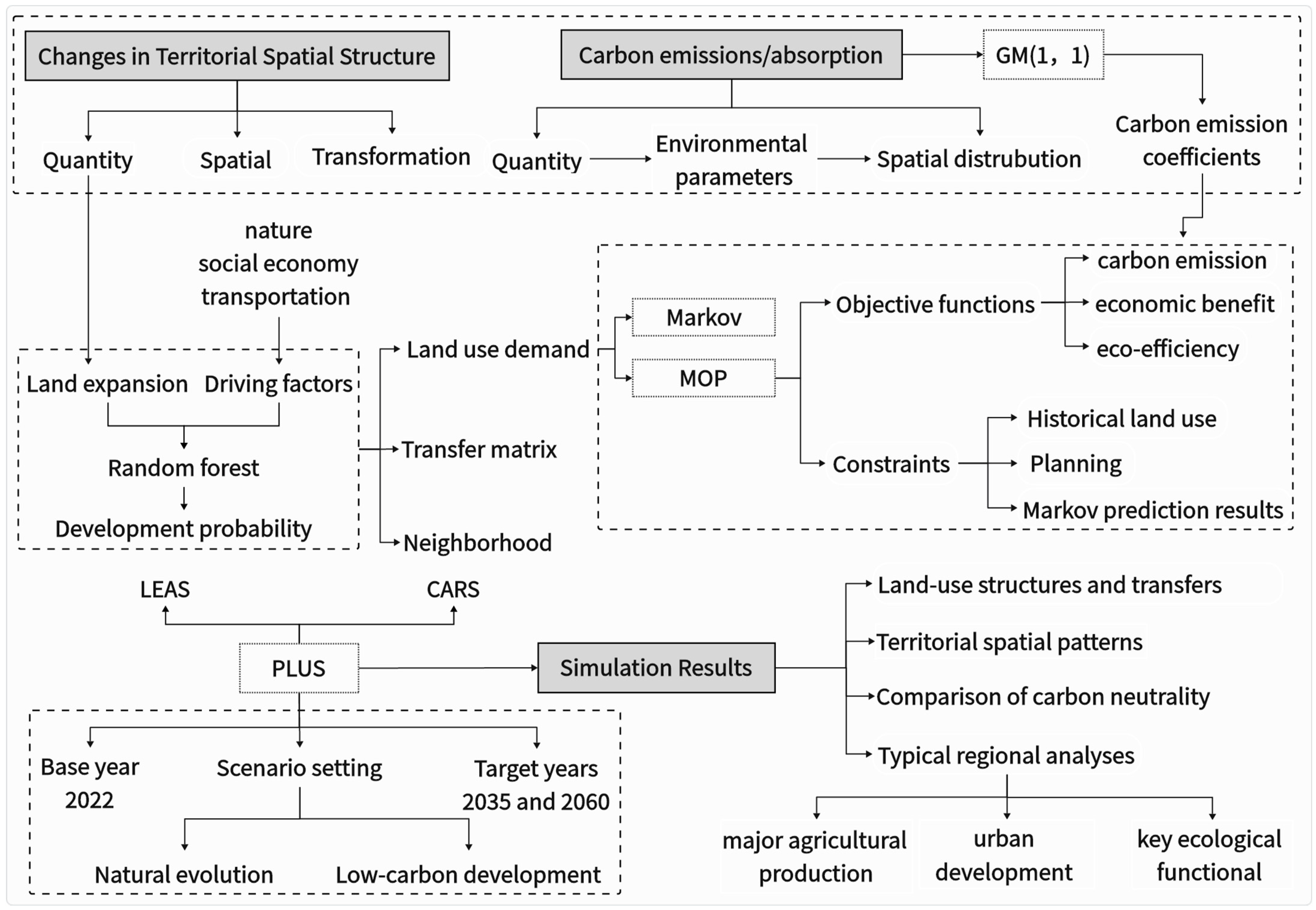
2.3. Research Framework

In this paper, the spatial data of land use in Wuan from 2012 to 2022 were used as the basis to analyze the changes in the territorial spatial structures and the land use flow during the decade. Using the carbon emission factor method, the carbon emissions/absorption of each category were calculated. Combined with environmental parameters, the spatial distribution of land use carbon emissions during the decade was obtained. Two scenarios of natural evolution and low-carbon development were set to simulate the territorial spatial structures in the future, taking the land use situation in 2022 as the initial year data and the target year of the new round of territorial spatial planning (2035) and carbon neutrality (2060) as the target years of land use simulation. Markov was used to obtain the land use demand data in the natural evolution scenario. MOP set three objectives of minimizing carbon emissions, maximizing financial benefits, and maximizing eco-efficiency and was used to obtain the land use demand data in the low-carbon development scenario. Comparing the carbon neutrality of the simulation results and the planning targets for 2035 reveals the role of territorial spatial planning on low-carbon development and provides suggestions for the future implementation of low-carbon development strategies for land use. The research framework is shown in Figure 2.

2.4. Quantifying Carbon Emissions/Absorption

Carbon emissions were calculated as positive (+) and carbon absorption as negative (−) in this study, and the sum of the two parameters represented the total carbon emissions. Research has indicated that farmland simultaneously has both carbon source and sink effects [46].

2.4.1. Carbon Emissions of Construction Land

The United Nations Intergovernmental Panel on Climate Change (IPCC, 2006) employed a technique to determine carbon emissions. This methodology was adopted in this study to account for carbon emissions from construction land. In other words, carbon emissions were projected on the basis of the consumption of various types of energy, the average low-level heat generation of various types of energy, the carbon emission coefficients of various types of energy, and the oxidation rate [18]. The formula for calculation is as follows:

$${\mathrm{E}}_{\mathrm{i}}=\sum _{\mathrm{i}=1}^6{\mathrm{C}}_{\mathrm{i}}\times {\mathrm{N}\mathrm{C}\mathrm{V}}_{\mathrm{i}}\times {\mathsf{\delta }}_{\mathrm{i}}\times {\mathrm{O}\mathrm{R}}_{\mathrm{i}}$$

(1)

${\mathrm{E}}_{\mathrm{i}}$ is the terminal carbon emissions from fossil energy; ${\mathrm{C}}_{\mathrm{i}}$ is the energy consumption; ${\mathrm{N}\mathrm{C}\mathrm{V}}_{\mathrm{i}}$ is the average low-level heat output, which refers to the China Energy Statistics Yearbook; ${\mathsf{\delta }}_{\mathrm{i}}$ is the ${\mathrm{C}\mathrm{O}}_2$ emission factor, which refers to the guidelines proposed by the IPCC (2006); ${\mathrm{O}\mathrm{R}}_{\mathrm{i}}$ is the oxidation rate of energy combustion; and $\mathrm{i} (1,2\dots 6)$ is the type of energy. In the actual calculation, more precise parameters were determined based on the research of related scholars [47]. The specific parameters are shown in

Table 2. Coefficient of different energy sources.

Type	${\mathbf{N}\mathbf{C}\mathbf{V}}_{\mathbf{i}}$ (TJ/104 t)	${\mathsf{\delta }}_{\mathbf{i}}$ (tC/TJ)	${\mathbf{O}\mathbf{R}}_{\mathbf{i}}$
coals	209.08	25.8	0.98
coke	263.44	29.2	0.98
oven gas	1735	12.1	0.995
petroleum	3893.1	15.3	0.995
petrol	430.7	20.2	0.99
diesel oil	426.25	20.2	0.99

.

2.4.2. Carbon Emissions of Farmland

The calculation of carbon emissions involves multiplying the consumption of different agricultural substances by their respective carbon emission factors, usually including fertilizers, pesticides, mulch, diesel, agricultural machinery, and so on [48]. In this study, the list of agricultural materials determined by relevant scholars was a reference [49,50], and the coefficient method for carbon emission accounting, which is based on clarifying carbon sources, was adopted [51]. The carbon emissions produced by farmland mainly originate from agricultural production activities. The formula for calculation is as follows:

$${\mathrm{E}}_{\mathrm{m}}=\sum {\mathrm{T}}_{\mathrm{m}}·{\mathsf{\gamma }}_{\mathrm{m}}$$

(2)

${\mathrm{E}}_{\mathrm{m}}$ represents the carbon emissions of farmland; ${\mathrm{T}}_{\mathrm{m}}$ is the volume of agricultural production activities; ${\mathsf{\gamma }}_{\mathrm{m}}$ is the coefficient of agricultural production activities; and $\mathrm{m} (1,2\dots )$ is the type of agricultural production activities. The carbon emission coefficients of each agricultural production activity are shown in

Table 3. Carbon emission factors of various agricultural production activities.

Type	Carbon Emission Factor
agricultural fertilizers (t/kg)	8.956 × 10−4
pesticides (t/kg)	4.934 × 10−3
agricultural plastic film (t/kg)	5.180 × 10−3
agricultural irrigation (t/hm2)	2.048 × 10−2
agricultural machinery (t/kw)	1.800 × 10−4

.

2.4.3. Carbon Absorption of Farmland

The calculation of carbon absorption primarily involves mathematically modeling the biomass and carbon sequestration rates of different crops [52]. Crops play a crucial role in reducing climate change, and there are variations in the carbon sequestration rates of different crops [53,54]. Concerning the research of related scholars, the carbon sequestration of farmland was estimated via the biological yield of crops and cash crops and the carbon sequestration coefficient of the reproductive period. The formulas are as follows:

$${\mathrm{S}}_{\mathrm{n}}={\mathrm{C}}_{\mathrm{n}}\times {\mathrm{D}}_{\mathrm{n}}$$

(3)

${\mathrm{S}}_{\mathrm{n}}$ is the ${\mathrm{C}\mathrm{O}}_2$ uptake of a certain crop; ${\mathrm{C}}_{\mathrm{n}}$ is the ${\mathrm{C}\mathrm{O}}_2$ uptake coefficient; ${\mathrm{D}}_{\mathrm{n}}$ is the biological yield; and $\mathrm{n} (1,2\dots )$ is the type of crops. The biological yield data were obtained from the Wuan Statistical Yearbook. Referring to related research results [55], the carbon absorption coefficients of major crops in China are shown in

Table 4. The carbon absorption coefficient of major crops and cash crops in China.

Type	Barley	Sorghum	Millet	Soya	Potatoes	Oilseeds	Vegetables	Wool	Tobacco	Fruits
${\mathrm{C}}_{\mathrm{n}}$	0.49	0.47	0.45	0.45	0.42	0.45	0.40	0.45	0.45	0.45

.

2.4.4. Carbon Absorption of Other Categories

The carbon absorption of other categories from 2012 to 2022 was calculated via the “carbon emission coefficient × area of land type”. Referring to the related research of other scholars, the carbon emission coefficients were corrected by combining the actual vegetation type, climate, soil, and other conditions in Wuan city.

Jingyun Fang calculated the absorption of carbon by vegetation in China from 1949 to 2003 [56,57] and reported that the average carbon emission coefficient of forest during the study period was −0.56. The mean carbon emission coefficient of scrubland was −0.134, whereas that of grassland was −0.021. In existing studies, scholars typically use direct coefficients for carbon emission estimation, which are basically −0.6 for forest and −0.02 for grassland. The city of Wuan is part of the North China flora–semiarid forest grassland vegetation system. Woody plants are dominated by shrubs, and there are fewer woodlands. Therefore, the carbon sink capacity of forest in Wuan should be slightly lower than the average level. On the basis of the above considerations, the carbon emission coefficient of forest in this study was set to −0.5. In the long term, the biomass of grassland vegetation in China has not changed much, and Hebei Province is at the average level in the whole country [58]. Therefore, the carbon emission factor for grassland was set to −0.02. The area of water and unused land in Wuan city is so small that it has little influence on overall carbon emissions. CO₂ from these two types of land has remained stable for a long time. Therefore, the carbon emission coefficients of these two types of land were determined to be −0.045 and −0.005, respectively, according to the results of existing research.

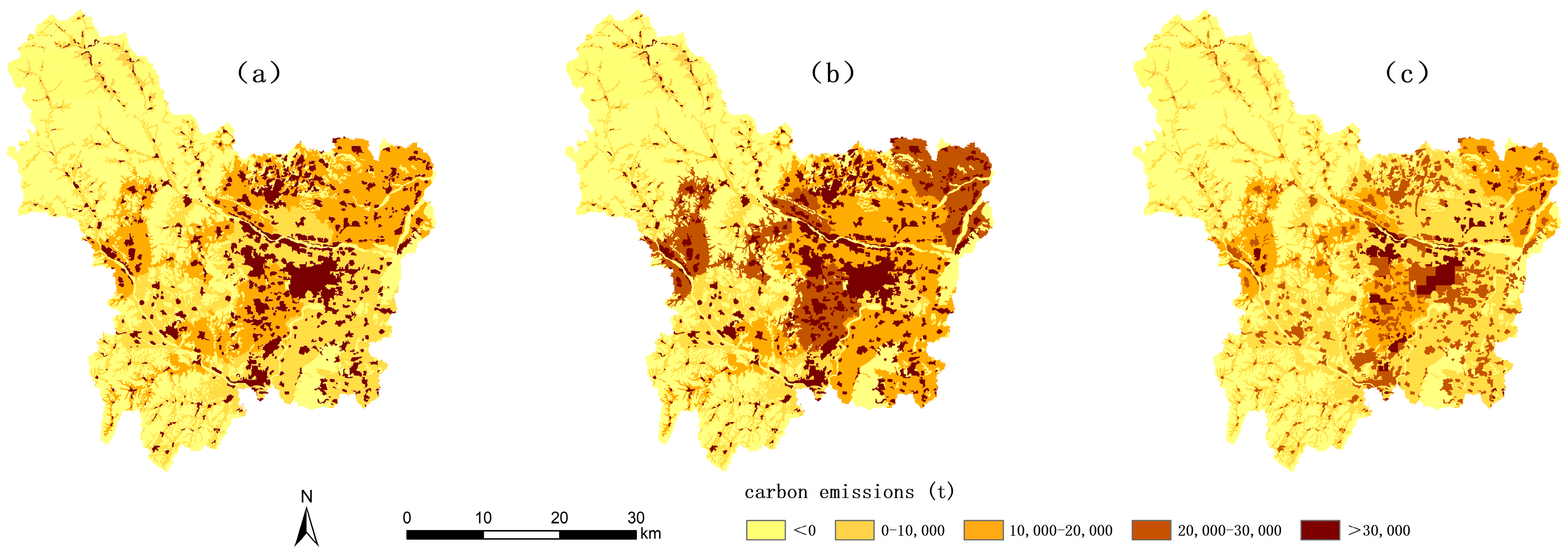
2.5. Spatial Distribution of Carbon Emissions/Absorption

To estimate the spatial distribution of carbon emissions/absorption, environmental parameters were introduced to capture spatially explicit information [59]. The curve fitting module in SPSS 27.0 was utilized to fit the functional relationship between each environmental parameter and the kernel density of each type of land use. The spatial distribution of carbon emissions/absorption was obtained from this correlation. The reasons for the selection of each environmental parameter and the rules for handling them are described below:

Relevant studies have shown that agricultural mechanization is the primary contributor to carbon emissions from farmland [60,61]. Consequently, the spatial estimation of carbon emissions from farmland needs to consider factors such as farmland size, grain yield, irrigated area efficiency, and the overall value of agricultural output. On the basis of the above factors, farmland was evaluated, and the evaluation results were used as environmental parameters for the spatialization of farmland carbon emissions. Many studies have shown a substantial influence of energy usage intensity on surface temperature [62]. Therefore, carbon emissions from construction land were allocated to each raster, depending on the geographical spread of the LST. The NDVI serves as an indicator of the growth conditions and extent of vegetation cover, both of which are important factors affecting the carbon sinks of vegetation [63]. Therefore, the NDVI was used as the standard to assign the carbon emissions of forest and grassland to the raster. Continuous reservoir construction has caused the originally free-flowing rivers to exhibit lake-like characteristics, which makes aquatic plants grow more easily. Therefore, the carbon sinks of reservoirs and pits should be greater than those of rivers. On the basis of the above characteristics and the water quality testing data from Wuan, a comprehensive evaluation of the water was conducted. The evaluation results were used as an environmental parameter for the spatialization of water carbon emissions. Since the area and the carbon sink coefficient of unused land are small, spatial differences were ignored and distributed evenly across each raster.

2.6. Forecasting the Land-Use Demand

2.6.1. Markov

Markov plots were used to forecast the land-use demands in 2035 and 2060 under the natural evolution scenario [64,65]. On the basis of this matrix, land-use demands for the next period can be predicted. The formulas describing the probability of land use transfer over time are as follows:

$${\mathrm{P}}_{\mathrm{i}\mathrm{j}}={\displaystyle \frac{{\mathrm{n}}_{\mathrm{i}\mathrm{j}}}{{\mathrm{n}}_{\mathrm{i}}}}$$

(4)

$${\mathrm{P}}_{\mathrm{i}\mathrm{j}}=\left[\begin{array}{cccc}{\mathrm{P}}_{11}& {\mathrm{P}}_{12}& \dots & {\mathrm{P}}_{1\mathrm{k}}\\ {\mathrm{P}}_{21}& {\mathrm{P}}_{22}& \dots & {\mathrm{P}}_{2\mathrm{k}}\\ ⋮& ⋮& \ddots & ⋮\\ {\mathrm{P}}_{\mathrm{k}1}& {\mathrm{P}}_{\mathrm{k}2}& \dots & {\mathrm{P}}_{\mathrm{k}\mathrm{k}}\end{array}\right]$$

(5)

$$0\le {\mathrm{P}}_{\mathrm{i}\mathrm{j}}\le 1, \sum _{\mathrm{j}=1}^{\mathrm{k}}{\mathrm{P}}_{\mathrm{i}\mathrm{j}}=1\left(\mathrm{I}, \mathrm{j}=1,2,3,\dots ,\mathrm{k}\right)$$

(6)

${\mathrm{n}}_{\mathrm{i}}$ denotes the number of pixels in which land use category $\mathrm{i}$ has changed; ${\mathrm{n}}_{\mathrm{i}\mathrm{j}}$ denotes the count of pixels that have undergone transformation from category $\mathrm{i}$ to category $\mathrm{j}$; and $\mathrm{k}$ denotes the land use type. The land use status at moment $\mathrm{t}({\mathrm{S}}_{\mathrm{t}})$ can be predicted from the land use status at moment $\mathrm{t}+1({\mathrm{S}}_{\mathrm{t}+1})$:

$${\mathrm{S}}_{\mathrm{t}+1}={\mathrm{S}}_{\mathrm{t}}\times {\mathrm{P}}_{\mathrm{i}\mathrm{j}}$$

(7)

2.6.2. MOP

MOP enables the identification of the best land-use framework across various policies and scenarios that can improve regional sustainable development and can help decision-makers determine future management goals and sensible land policies [66]. MOP was used to forecast the land-use demands in 2035 and 2060 under the low-carbon development scenario; this scenario contained three parts, namely, model variables, constraints, and an objective function, which is expressed as follows:

$$\sum _{\mathrm{j}=1}^{\mathrm{n}}{\mathrm{a}}_{\mathrm{i}\mathrm{j}}{\mathrm{X}}_{\mathrm{i}}={\mathrm{b}}_{\mathrm{j}}\left(\mathrm{i}=1,2,3,\dots ,\mathrm{n}\right)$$

(8)

The objective function is $\mathrm{F}\left(\mathrm{x}\right)={\sum }_{\mathrm{j}=1}^{\mathrm{n}}{\mathrm{C}}_{\mathrm{j}}{\mathrm{X}}_{\mathrm{j}}=\mathrm{m}\mathrm{a}\mathrm{x} (\mathrm{o}\mathrm{r} \mathrm{m}\mathrm{i}\mathrm{n})$, and the solution $\left\{{\mathrm{X}}_{\mathrm{j}}\right\}$ obtained by the equation emerges as the best possible solution. ${\mathrm{X}}_{\mathrm{j}}$ is the area of each category; ${\mathrm{C}}_{\mathrm{j}}$ is the coefficient of each category under the unit area.

• Model variables

Six independent variables were set in this study, with 2022 as the base period (X₁: farmland, X₂: forest, X₃: grassland, X₄: water, X₅: construction land, X₆: unused land).

2.

Constraints

Constraints were formulated on the basis of the data for land-use demand under the natural evolution scenario, Wuan Territorial Spatial Planning (2021–2035), and the requirements of low-carbon development (

Table 5. Constraints.

Type	Constraints		Instruction
	2035	2060
total area	${\displaystyle \sum _{\mathrm{i}=1}^6}{\mathrm{X}}_{\mathrm{i}}=\mathrm{181,805}$	${\displaystyle \sum _{\mathrm{i}=1}^6}{\mathrm{X}}_{\mathrm{i}}=\mathrm{181,805}$	According to the Wuan Territorial Spatial Planning (2021–2035) (from now on referred to as spatial planning), the total planning area is 181,805 hm2.
variables	${\mathrm{X}}_{\mathrm{i}}>0, \mathrm{i}=1,2,3,4$	${\mathrm{X}}_{\mathrm{i}}>0, \mathrm{i}=1,2,3,4$	Each type of land use must not be a negative area.
farmland	${\mathrm{X}}_1\ge \mathrm{51,022}$	${\mathrm{X}}_1\ge \mathrm{49,294}$	According to the spatial planning, the farmland area in 2035 will not be less than 51,022 hm2, which is used as the lower limit in 2035. The Markov projection is taken as the lower limit of the farmland area in 2060.
forest	$\mathrm{60,351}\le {\mathrm{X}}_2\le \mathrm{69,404}$	$\mathrm{61,627}\le {\mathrm{X}}_2\le \mathrm{70,871}$	Forest, as the most important carbon sink, should become more afforested in the future. The Markov projections were used as the lower limit of forest area in both 2035 and 2060, with a 15% increase as the higher limit.
grassland	$\mathrm{28,867}\le {\mathrm{X}}_3\le \mathrm{30,919}$	$\mathrm{28,478}\le {\mathrm{X}}_3\le \mathrm{29,022}$	According to the spatial planning, grassland will be reduced to utilize the benefits of the land. Markov projections are used as the lower limit. The 2022 grassland area is the higher limit of 2035. The 2035 MOP projection is the higher limit of that of 2060.
water	$5062\le {\mathrm{X}}_4\le 5226$	$4422\le {\mathrm{X}}_4\le 4913$	The water area will be reduced. Markov projections are used as higher limits. The spatial planning goal is the lower limit of water area in 2035. The water area in 2060 is the lower limit via a 10% reduction in the Markov projection.
construction land	${\mathrm{28,534}\le \mathrm{X}}_5\le \mathrm{35,730}$	${\mathrm{29,916}\le \mathrm{X}}_5\le \mathrm{36,695}$	Construction land needs to be strictly controlled. The construction land areas in 2035 and 2060 are capped by Markov projections. The 2022 construction land area is the lower limit of 2035. The spatial planning goal is the lower limit of construction area in 2060.
unused land	$896\le {\mathrm{X}}_6\le 1101$	$806\le {\mathrm{X}}_6\le 896$	According to spatial planning, the efficiency of land use will be improved, so the unused land area will be reduced. The unused land area in 2035 will be capped by 2022, with the planning target as the lower limit. The area of unused land in 2060 will be capped by the planning target in 2035, with the planning target of a 10% reduction as the lower limit.

). Strict regulation is necessary for construction land, which is the primary contributor to carbon emissions. Forest needs to be restricted from being converted to construction land and other agricultural land.

3.

Multi-objective function

For the feasibility of the multi-objective approach, the goals set were to reduce carbon emissions while enhancing economic and ecological advantages. Three objective functions were collated into a combined function F(x). Following the resolution of each objective function for 2035 and 2060, the objective function was divided by its corresponding value, after which a collective solution was executed. The formula is as follows:

$$\mathrm{F}(\mathrm{x})={\mathrm{W}}_1{\displaystyle \frac{{\mathrm{F}}_1\left(\mathrm{x}\right)}{{\mathrm{G}}_1}}-{\mathrm{W}}_2{\displaystyle \frac{{\mathrm{F}}_2\left(\mathrm{x}\right)}{{\mathrm{G}}_2}}+{\mathrm{W}}_3{\displaystyle \frac{{\mathrm{F}}_3\left(\mathrm{x}\right)}{{\mathrm{G}}_3}}$$

(9)

${\mathrm{G}}_1, {\mathrm{G}}_2, {\mathrm{G}}_3$ are the target values of the financial benefit, carbon emission, and eco-efficiency functions, respectively; ${\mathrm{W}}_1, {\mathrm{W}}_2, {\mathrm{W}}_3$ are the weight coefficients of the corresponding functions, which are 0.2, 0.7, and 0.1, respectively. At this point, the constraints on the objective function of carbon emissions are greater, and the results have greater effects on carbon sink enhancement.

(1)

Coefficients of the carbon emission objective function

According to the method of calculating the carbon emissions/absorption in Section 2.3, the yearly carbon emissions of construction land and farmland from 2012 to 2022 can be obtained. The yearly carbon emission coefficient can be obtained by calculating the “carbon emissions/area of land type”. The carbon emission factors in the target years 2035 and 2060 were calculated via GM (1, 1). According to Section 2.4.4, the carbon emission coefficients of other types of land use in the target years, 2035 and 2060, were determined to be −0.5, −0.02, −0.045, and −0.005, respectively.

(2)

Coefficients of the financial benefit objective function

The coefficients of the financial benefit of each land use in the target year were calculated via GM (1, 1), accounting for the per unit area economic output of each category from 2012 to 2022. Agricultural production, forestry production, pastoral production, fishery production, and secondary and tertiary industry values were used to quantify the financial benefits of farmland, forest, grassland, water, and construction land, respectively. The financial benefit of unused land was not calculated.

(3)

Coefficients of the eco-efficiency objective function

Eco-efficiency is usually quantified by market prices or the cost of alternative products and services [67,68]. Utilizing Gaodi Xie’s equivalent factor method, a chart detailing equivalent factors for ecosystem service value in Wuan was created [69]. The eco-efficiency for each category per unit area was calculated as a standard equivalent of the economic value of natural food production for 1 hm² of farmland per year, with an average national yield. The eco-efficiency coefficients for each site in 2035 and 2060 were obtained via GM (1, 1). The objective functions of the financial benefit ${\mathrm{F}}_1\left(\mathrm{x}\right)$, carbon emission ${\mathrm{F}}_2\left(\mathrm{x}\right)$, and eco-efficiency ${\mathrm{F}}_3\left(\mathrm{x}\right)$ are shown in

Table 6. Multi-objective function expressions for the low-carbon development scenario.

Year	Function Expression
2035	financial benefit: ${\mathrm{F}}_1\left(\mathrm{x}\right)=13.41{\mathrm{x}}_1+0.95{\mathrm{x}}_2+20.77{\mathrm{x}}_3+117.92{\mathrm{x}}_4+1196.84{\mathrm{x}}_5+{\mathrm{x}}_6=\mathrm{m}\mathrm{a}\mathrm{x}$ carbon emission: ${\mathrm{F}}_2\left(\mathrm{x}\right)=1.66{\mathrm{x}}_1-0.5{\mathrm{x}}_2-0.02{\mathrm{x}}_3-0.045{\mathrm{x}}_4+9.79{\mathrm{x}}_5-0.005{\mathrm{x}}_6=\mathrm{m}\mathrm{i}\mathrm{n}$ eco-efficiency: ${\mathrm{F}}_3\left(\mathrm{x}\right)=1.55{\mathrm{x}}_1+10.4{\mathrm{x}}_2+8.88{\mathrm{x}}_3+56.62{\mathrm{x}}_4-6.43{\mathrm{x}}_5+0.05{\mathrm{x}}_6=\mathrm{m}\mathrm{a}\mathrm{x}$
2060	financial benefit: ${\mathrm{F}}_1\left(\mathrm{x}\right)=20.55{\mathrm{x}}_1+1.03{\mathrm{x}}_2+18.75{\mathrm{x}}_3+132.88{\mathrm{x}}_4+1579.64{\mathrm{x}}_5+{\mathrm{x}}_6=\mathrm{m}\mathrm{a}\mathrm{x}$ carbon emission: ${\mathrm{F}}_2\left(\mathrm{x}\right)=0.82{\mathrm{x}}_1-0.5{\mathrm{x}}_2-0.02{\mathrm{x}}_3-0.045{\mathrm{x}}_4+7.25{\mathrm{x}}_5-0.005{\mathrm{x}}_6=\mathrm{m}\mathrm{i}\mathrm{n}$ eco-efficiency: ${\mathrm{F}}_3\left(\mathrm{x}\right)=1.03{\mathrm{x}}_1+12.65+7.46{\mathrm{x}}_3+62.73{\mathrm{x}}_4-8.34{\mathrm{x}}_5+0.03{\mathrm{x}}_6=\mathrm{m}\mathrm{a}\mathrm{x}$

.

2.7. Simulation of Territorial Space

After completing the forecast for land-use demand, the obtained values were used as constraints on the land-use demand to simulate the territorial spatial distribution of Wuan in 2035 and 2060 through the PLUS model.

2.7.1. Factors Driving Land-Use Change

Studies focusing on the factors influencing land-use change, both domestically and internationally, have progressed considerably. It is found that economic, social, population, and natural factors play a dominant role in urban expansion based on the extent to which impacts range from significant to minor [70]. Human-induced factors have always been the most significant contributors to land-use change, surpassing the impact of natural causes, with transportation and business services emerging as key influencers. However, the influence of natural conditions, such as topography, on land-use change persists [71]. Concerning domestic and international studies on the mechanism driving land-use change and research results related to land-use scenario simulation [72], nine influential factors were selected from the perspectives of nature, socioeconomics, and transport accessibility. They were unified into a 30 m × 30 m raster via tools such as the mosaic, project, and resample tools in ArcGIS 10.8. The normalized driving data are shown in Figure 3.

2.7.2. Configuration of Parameters under Different Scenarios

The main parameters of PLUS include the demands for land use, transfer matrix, and neighborhood weights. On the basis of the methodology described in Section 2.5, the demands for land use were obtained and are shown in

Table 7. Demands for land use.

Year	Scenario	Farmland	Forest	Grassland	Water	Construction Land	Unused Land
2035	Natural evolution	50,605	60,351	28,867	5226	35,730	1026
	Low-carbon development	51,802	66,406	29,022	5062	28,616	897
2060	Natural evolution	49,294	61,627	28,478	4913	36,695	798
	Low-carbon development	50,523	67,030	28,573	4900	29,930	849

.

The transfer matrix parameter is set to either “1” or “0”, where “1” signifies permissible transfers between two types of land use and “0” denotes the prohibition of such transfers (

Table 8. Transfer matrix.

Type	Natural Evolution Scenario						Low-Carbon Development Scenario
	a	b	c	d	e	f	a	b	c	d	e	f
a	1	1	1	1	1	1	1	1	0	1	1	0
b	1	1	1	1	1	1	1	1	1	1	0	0
c	1	1	1	1	1	1	1	1	1	1	1	1
d	1	1	1	1	0	1	1	1	1	1	0	1
e	0	0	0	0	1	0	0	0	0	0	1	0
f	1	1	1	1	1	1	1	1	1	1	1	1

a: farmland, b: forest, c: grassland, d: water, e: construction land, f: unused land.

). The nature reserves of Wuan consist of the Qingyazhai National Nature Reserve, Wuan National Forest Nature Park, and Congtai Zishan Provincial Forest Nature Park, with a total area of 384.41 km². The area of permanent basic farmland is 545.25 km². Permanent basic farmland and nature reserves were included in the PLUS as restrictions on the transformation areas.

The range of values for the neighborhood weight is “0~1”, and a larger value indicates a greater influence of the neighborhood. The neighborhood weights were set considering the ratio of each land use expansion type relative to the overall land area from 2012 to 2022, accounting for the requirements of the scenarios and relevant research findings (

Table 9. Neighborhood weights.

Scenario	Farmland	Forest	Grassland	Water	Construction Land	Unused Land
Natural evolution	0.40	0.55	0.45	0.25	0.95	0.10
Low-carbon development	0.30	0.75	0.60	0.30	0.80	0.10

).

3. Results

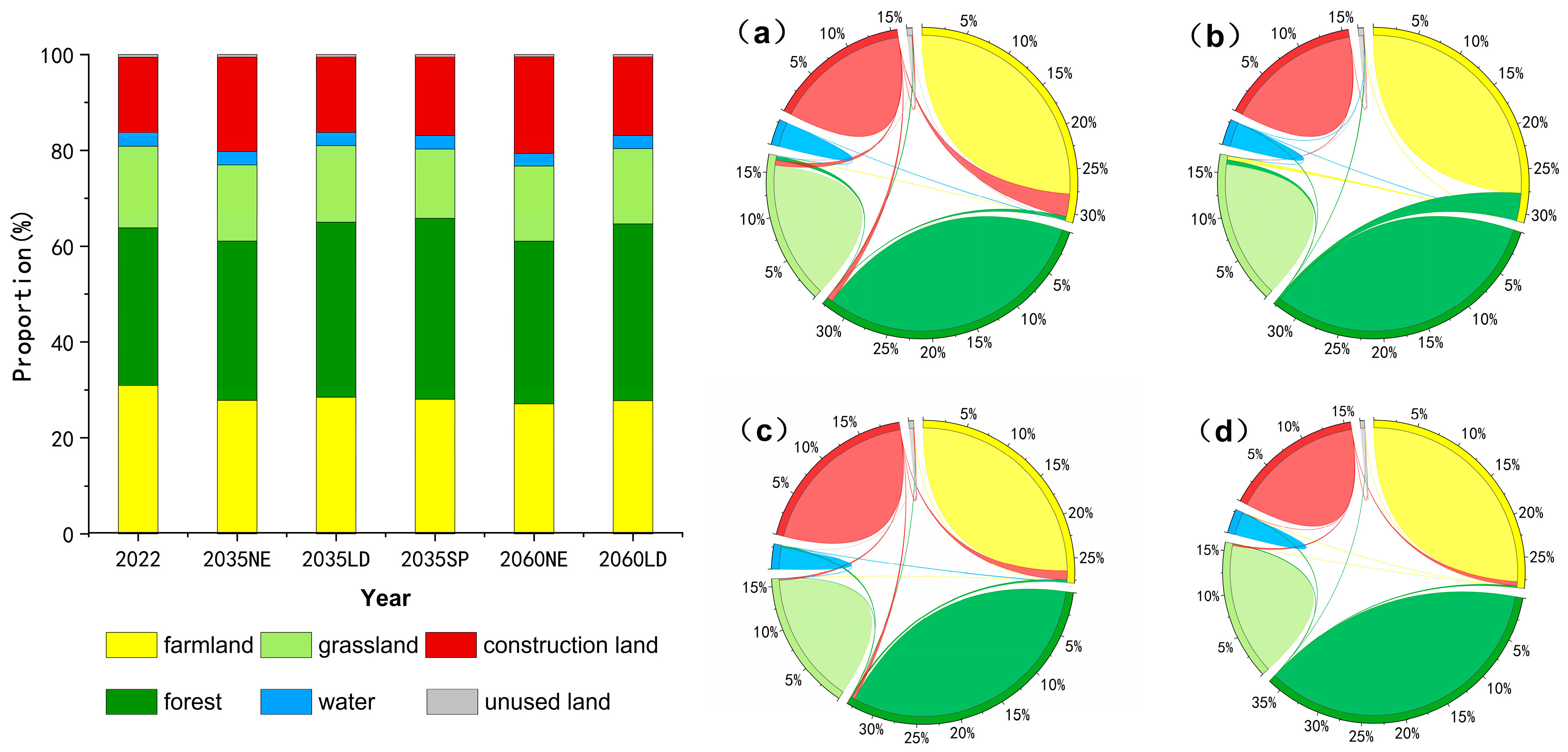
3.1. Changes in Territorial Spatial Structure

The territorial spatial patterns from 2012 to 2022 are shown in Figure 4. Spatially, the land-use types in Wuan are predominantly farmland and forest, which account for more than 60% of the total area. Forest and grassland are concentrated in the northwestern and southwestern parts, respectively. Farmland is distributed over a large area in the entire central region. The city’s central area predominantly features construction land, which is intermittently allocated nearby. Water is distributed in a band throughout the entire study area. Unused land is sporadically distributed in the study area.

The land-use transfer situation is shown in Figure 5. There was swift expansion in the expansion of construction land, and the areas of farmland, grassland, and water all decreased to varying degrees, with farmland and grassland decreasing the fastest. Forest and unused land showed a trend of decreasing and then increasing. This is because since entering the 21st century, China’s urbanization and industrialization have been accelerating, and urban construction land and industrial land have taken up a large amount of farmland as well as ecological land. Forest was decreasing until 2019, and after 2019, the area of forest started to increase due to the increased efforts of returning farmland to forest and afforestation. The transfer area from 2017 to 2022 was significantly larger than that from 2012 to 2017. The conversion of farmland to construction land was the most dominant type of transfer from 2012 to 2017, accounting for 0.52% of the total area. This was followed by the mutual transfer of grassland and farmland, each accounting for about 0.4% of the total area. In 2017–2022, the conversion of farmland to construction land was the most dominant type of transfer, accounting for 1.68% of the total area. This was followed by the mutual transfer of grassland and farmland, each accounting for about 0.75% of the total area. In addition, the two transfer types of farmland to forest and grassland to forest were also more important, accounting for 0.63% and 0.41% of the total area, respectively. Overall, the primary process of transforming land use involved moving farmland to construction land, along with exchanging farmland and grassland. The transformation of farmland to construction land accounted for 33.5% of all transformation types and was the dominant transformation type.

3.2. Patterns in Both Space and Time of Carbon Emissions

From 2012 to 2022, there was a pattern of increase and subsequent decrease in both net carbon emissions and carbon emissions (Figure 6a). As shown in Figure 6b, farmland and construction land manifested as carbon sources, and both types of carbon emissions fluctuated, initially rising and subsequently falling. Before 2015, carbon emissions from construction land increased year by year, which was mainly due to the increased demand for construction land from urbanization and industrialization. According to the Wuan Statistical Yearbook, the consumption of energy sources, such as coal and coke, has been decreasing annually since 2015, and its proportion has decreased. However, the consumption and share of cleaner energy sources have increased. As a result, carbon emissions from construction land began to decrease year by year. Initially, agriculture was still in the traditional crude development stage, so carbon emissions continued to grow. In recent years, the volume of agricultural production activities, such as those involving agricultural fertilizers and diesel, has been greatly reduced in favor of green agriculture. Therefore, the carbon emissions from farmland began to decrease. Construction land is the most important carbon source in Wuan, and the carbon emissions from it have decreased by 35.71 × 10⁴ t in the past 10 years, accounting for a gradually decreasing proportion of total carbon emissions from carbon sources, from 76% to 68%. In contrast, the share of carbon emissions originating from farmland in the overall carbon emissions from carbon sources increases annually, from 24% to 32%. The carbon emissions from farmland have decreased by 5.92 × 10⁴ t during the past 10 years. Before 2015, there was a noticeable decline in carbon sinks, followed by a minor rise after 2015 due to increased efforts to return farmland to forest and afforestation. As the biological production of various crops and cash crops on farmland decreased after 2020, the number of carbon sinks began to decrease slightly. Forest is the most important carbon sink, accounting for 97% of the total carbon sequestered, assuming the most important role in carbon sequestration. An analysis of the results of the calculation reveals that carbon emissions depend mainly on the expansion of construction land and energy consumption. Compared with the measures to control the sources of carbon emissions, the carbon reduction potential of utilizing the carbon sequestration effect of natural land (forest and grassland) is limited. The city of Wuan should focus on controlling the total amount of energy consumed and adjusting the energy structure. In particular, reducing the proportion of coal consumption can effectively slow the increasing trend of carbon emissions.

Carbon emissions from 2012 to 2022 are divided into five classes, as shown in Figure 7. Carbon emissions radiate from the center and gradually weaken outward, generally exhibiting a pattern of elevated levels in the center and diminished levels on both sides. Areas with high carbon emissions predominantly cluster in the basin’s economically advanced regions, with central urban areas at their core. This is because the central urban area has a large construction land area, a large population and higher energy consumption. Most of the carbon-negative zones are in key ecological reserves in the northwestern and southwestern regions. This part of the region is dominated by natural land (woodland and grassland) with carbon sequestration functions and has a stronger carbon sink capacity. The majority of areas that emit more carbon are situated within the iron and steel industrial zone, which is dominated by coal mining and iron and steel production. Industrial land has a higher demand for energy consumption, which results in a large amount of carbon emissions. The spatial dynamic evolution reveals that from 2012 to 2017, areas exhibiting elevated carbon emissions demonstrated a notable increase, and from 2017 to 2022, regions with relatively high carbon emissions showed a sharp contractionary trend. This is inextricably linked to the implementation of China’s energy-saving and emission-reduction policies in recent years.

3.3. Simulation Results

3.3.1. Verification of the Model Accuracy

According to past land-use data and selected driving factors, the sample set was randomly sampled at a ratio of 1%. The random forest method was used for training to obtain expansion patterns for different land classes. According to the expansion probability of each land category, combined with various parameters and based on the land use data from 2012, the spatial distribution of land use in 2022 was obtained through PLUS. According to the accuracy calculations of the validation module with the PLUS model, the kappa coefficient is 0.87, and the overall accuracy (OA) is 0.91. The data indicate that the simulation accuracy of PLUS is high, which is in line with the development of land use and can be used to predict the trend of future land use development.

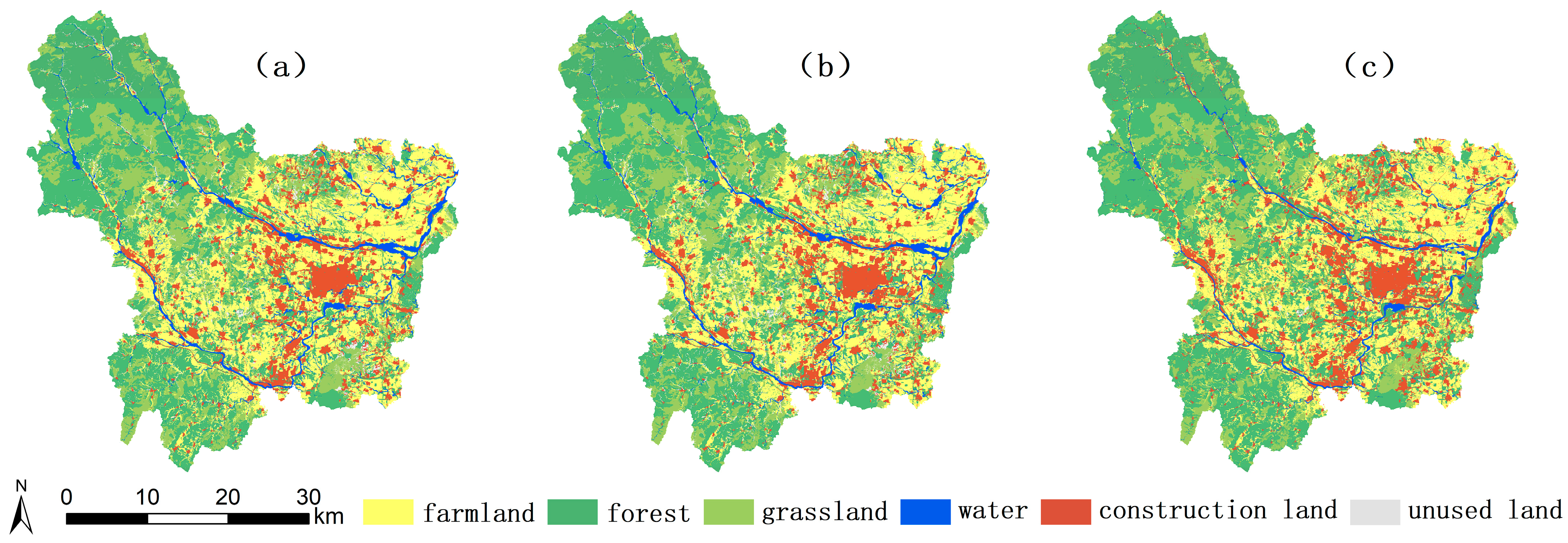
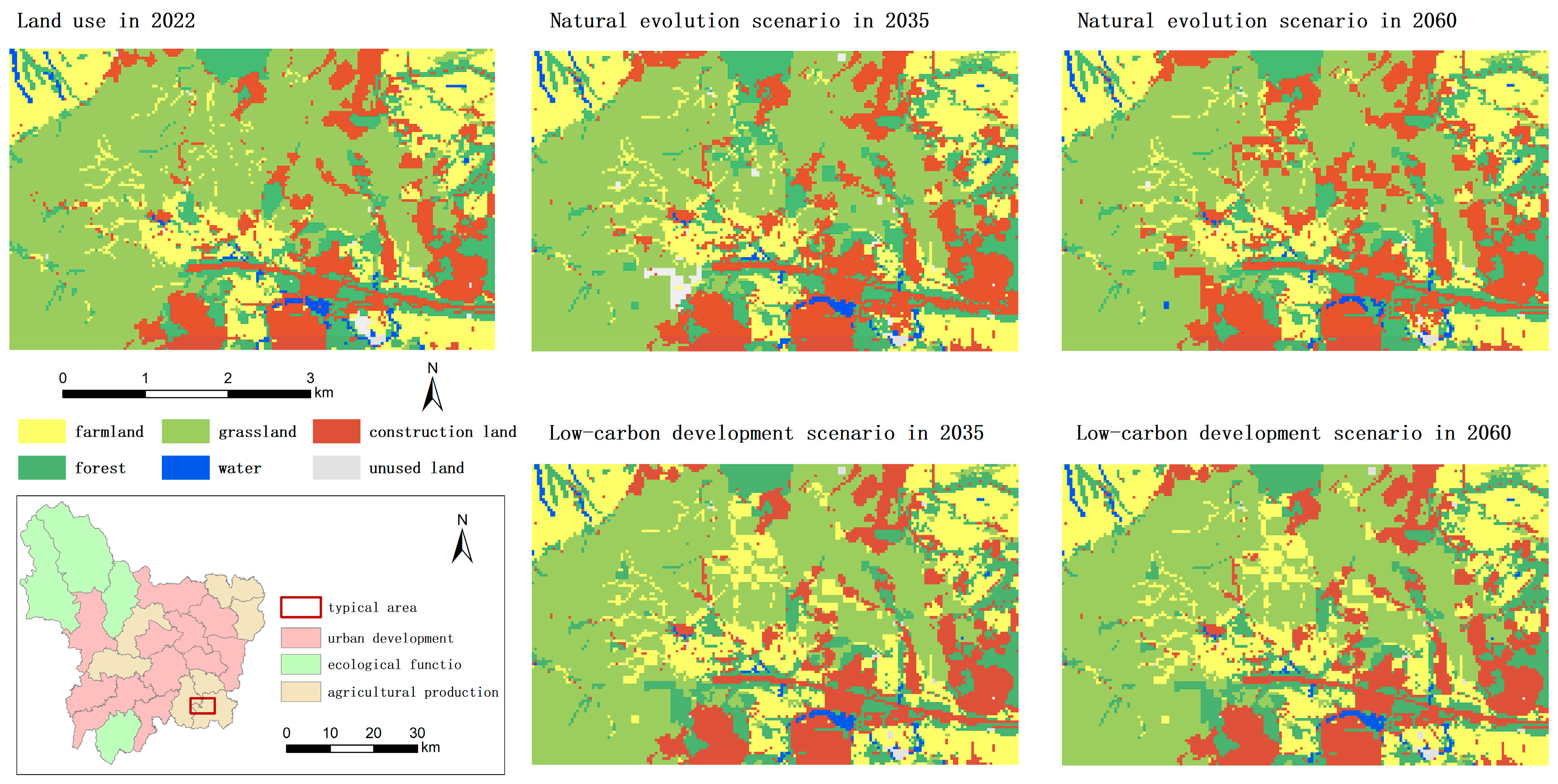
3.3.2. Territorial Spatial Patterns

After the model was validated and land-use demand was obtained, the territorial spatial patterns in 2035 and 2060 were simulated through the PLUS. The results are shown in Figure 8. In general, the territorial spatial patterns under the two scenarios are basically the same. In terms of development trends, both show either outward expansion or inward contraction along existing regions. Forest and grassland, which are key ecological functional areas, are largely distributed in the northwestern and southwestern regions at relatively high elevations. Farmland is distributed in low-elevation areas outside forest and grassland, as well as on both sides of the water. Three important water systems are distributed in the shape of a belt. The bulk of construction land is allocated to the economically advanced central region, with an occasional radial distribution in relation to the external area.

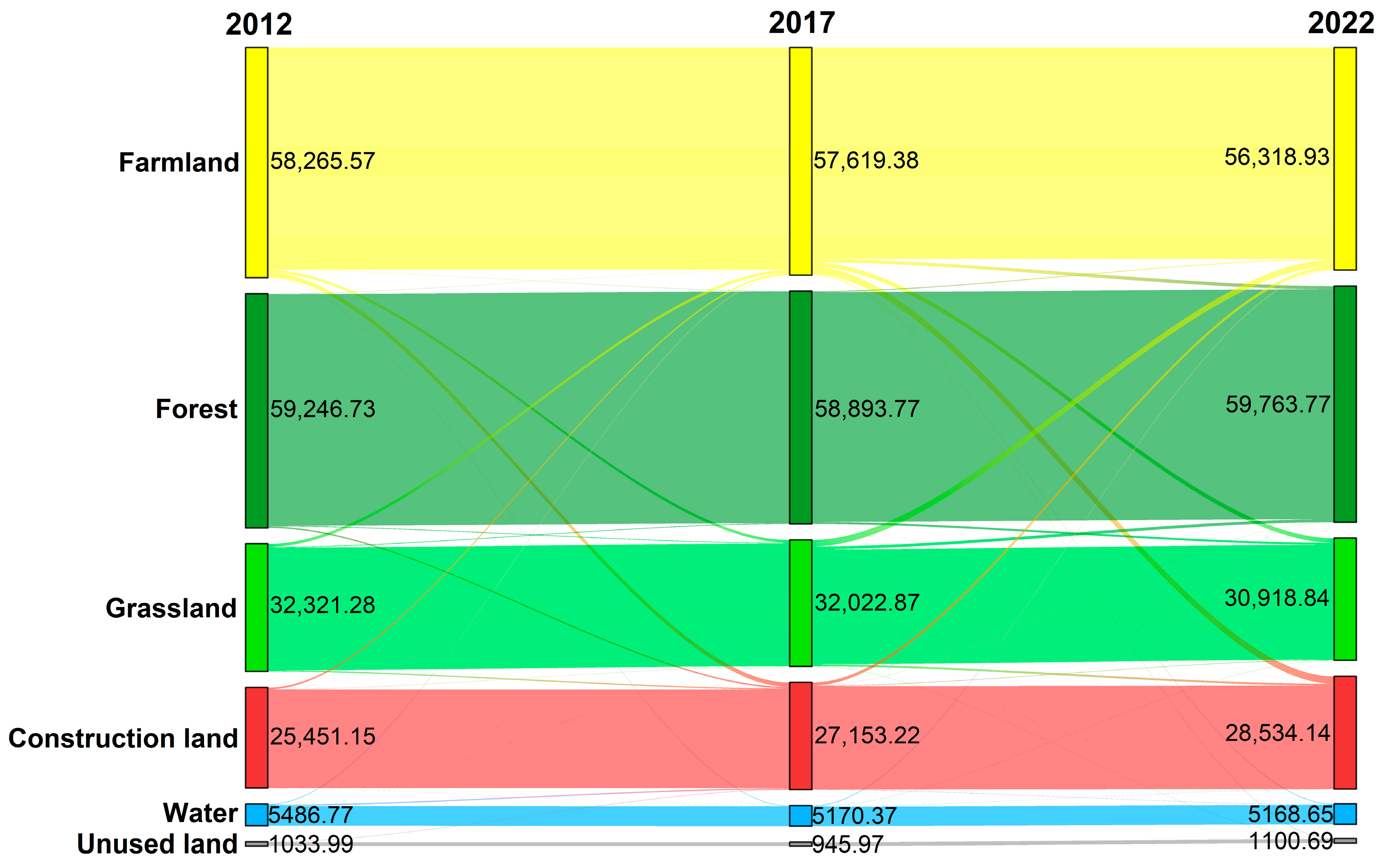
3.3.3. Land-Use Structures and Land-Use Transfers

As shown in Figure 9, the land-use structures under the two scenarios in 2035 and 2060 are similar to those in 2022. The land-use types are dominated by farmland and forest, each accounting for approximately 30% of the total area. These types are followed by construction land and grassland, both of which account for approximately 20% of the total area. Water accounts for approximately 2.8% of the total area, and unused land accounts for approximately 0.5% of the total area. Land types with lower economic benefits, such as farmland, grassland, and unused land, show a decreasing trend under both scenarios. This is because given the characteristics of historical land use changes, economic development has always been prioritized, and the construction land required for urban development is obtained mainly through the occupation of ecological land, as well as cropland, which results in continuous shrinkage of future urban ecological space and agricultural space.

The characteristics of the land-use transfers under the two scenarios are quite different. Under the natural evolution scenario in 2022–2060, the most important direction of transfer for all categories is construction land, the inflow area of which is 8353.48 hm², accounting for 4.59% of the total area. Among this area, the conversion of farmland into construction land represents the most extensive area, comprising 64.15% of the overall construction land inflow. The conversion of farmland to forest was the second-most important transfer, with a transfer area of 1753.12 hm², accounting for 0.96% of the total area. Under the low-carbon development scenario from 2022–2060, the most important transfer for all categories is forest. The inflow area of forest is 7737.55 hm², accounting for 4.26% of the total area. Among them, the region of farmland transformed into forest stands as the most extensive, comprising 79.87% of the overall incoming area of forest. Construction land and farmland are the second-most important inflow categories, representing 0.77% and 0.71% of the entire area, respectively.

3.3.4. Typical Regional Analyses

The spatial details of LUCC under the different scenarios were examined at the regional scale. According to the Wuan Territorial Spatial Planning (2021–2035), Wuan is divided into three main functional areas: major agricultural production areas, urban development areas, and key ecological functional areas. The geographical specifics of LUCC across various situations were analyzed regionally.

For the typical region of the major agricultural production areas (Figure 10), the southeastern region, where farmland is not concentrated, was selected. This area is at a slightly higher elevation than the surrounding area. The natural evolution scenario is dominated by the expansion of land used for construction, whereas the low-carbon development scenario is dominated by the expansion of farmland supplemented by the expansion of forest. This shows that the low-carbon development scenario is better able to guarantee food security in the major agricultural production areas.

For the typical region of the urban development areas (Figure 11), the area of northern construction land was selected for analysis. The ecological space is severely compressed, and construction land is significantly expanded in both scenarios. However, certain ecological land will be converted to farmland in the low-carbon development scenario, which shows that it has a lower risk of carbon emissions than does the natural development scenario.

For the typical region of the key ecological functional areas (Figure 12), the river penetration zone in the northwest corner was selected for analysis. The area is covered by large areas of forest, with a small amount of farmland and construction land present along the river. Since this area is a key ecological functional area and has an important guaranteed ecological function, the ecological space is not compressed under either scenario. In a scenario of natural evolution, the extent of land used for construction near a river expands incrementally, primarily through the transformation of farmland into construction land. In a scenario of low-carbon development, forest growth is gradual, primarily because of the transformation of farmland into forest.

3.4. Comparison of Carbon Neutrality

The carbon emissions for different scenarios in 2022, 2035, and 2060 were calculated (

Table 10. Carbon emissions in 2022, 2035, and 2060.

Year	Scenario	Farmland	Forest	Grassland	Water	Construction Land	Unused Land	Carbon Emissions
2022	status	150,782.67	−29,895.05	−617.94	−232.86	314,862.8	−5.51	434,894.12
2035	natural	84,004.33	−30,175.46	−577.34	−235.17	349,799.54	−5.13	402,810.77
	low-carbon	85,990.56	−33,203.01	−580.45	−227.79	280,151.03	−4.48	332,125.86
	planning	84,696.52	−34,286.00	−526.74	−227.79	292,877.64	−4.48	342,529.15
2060	natural	40,421.41	−30,813.46	−569.57	−221.06	266,037.13	−3.99	274,850.45
	low-carbon	41,429.03	−33,515.16	−571.45	−220.50	216,992.36	−4.24	224,110.04

). Under all the scenarios, there is a downward trajectory in net carbon emissions. Carbon emissions from all carbon sources decrease, except for an increase from construction land in the 2035 natural evolution scenario. There is a reduction in carbon absorption by grassland and unused land, whereas carbon absorption by forest and water increases. In 2035, the net carbon emissions projected by the natural evolution scenario will surpass those under the planning target and the low-carbon scenario. Territorial spatial planning is the basis for development and conservation efforts and represents the optimal strategy for realizing land-use optimization objectives [73]. In 2060, the net carbon emissions under the natural evolution scenario surpassed those under the low-carbon development scenario. Both scenarios do not reach carbon neutrality by 2060. However, under the low-carbon development scenario, the net carbon emissions are only half of those in 2022, with obvious carbon emission reduction effects. This suggests that land-use optimization measures that are consistent with the constraints of territorial spatial planning are more effective in facilitating the attainment of carbon neutrality objectives [74].

4. Discussion

4.1. Rationality of the Research Methodology

Earlier research has concentrated on low-carbon development strategies for land utilization or assessments of carbon effects under different land-use patterns [75,76,77,78]. This research elucidated how territorial spatial planning contributes to carbon neutrality by comparing the planning goals for 2035 with the modeling results. In addition, the contributions of other scenarios to carbon emission reduction were explored, with the aims of adjusting territorial spatial planning to achieve carbon neutrality and providing new perspectives for land use management. PLUS merges the benefits of transformation and pattern analysis strategies, outlining the characteristics of changes in land use over a designated period [79]. In summary, the PLUS results are more reliable and can simulate land-use changes at the patch level.

4.2. Interaction between Territorial Spatial Planning and Carbon Neutrality

The most central function of territorial spatial planning is its spatiotemporal orientation toward the future of land use, which must comply with the maximization of benefits requiring compliance with constraints [80]. The section on territorial spatial planning in Wuan Territorial Spatial Planning (2021–2035) focused primarily on the overall strategy as an initial step, which is a gray system with incomplete information. The impact of carbon reduction on planning targets surpasses that of the natural evolution scenario, underscoring the importance of territorial spatial planning. This is because territorial spatial planning is crucial for addressing issues such as the excessive and rapid reduction of farmland and the deterioration of ecosystem functions, which contribute to achieving carbon neutrality. However, compared with the low-carbon development scenario, the planning objectives do not consider carbon neutrality sufficiently. To reach its carbon neutrality goal, refining territorial spatial planning is crucial.

4.3. Correlations between Land-Use Change and Carbon Emissions

Cities have different development objectives and different impacts on territorial spatial structure [3]. Similar to previous studies [33], the scenario of natural evolution led to a swift increase in the size of construction land. The lack of a significant expansion in construction land area coupled with a greater extent of forest expansion in the scenario of low-carbon development suggests that low-carbon strategies play a crucial role in curbing urban sprawl. A significant link exists between the type of land use and the intensity of regional carbon emissions. The carbon sinks showed an increasing trend after 2015, mainly due to increased efforts to plant trees and return farmland to forest. Different developmental objectives and strategies can significantly impact land-use structures and functions, resulting in different degrees of human conduct, and consequently, variations in carbon emissions.

4.4. Pathways to Carbon Neutrality

Under the low-carbon development goal, the expansion of forest relies mainly on the transfer of farmland, contradicting the basic national strategy of “effectively protecting farmland”. Given the limited potential for forest and grassland expansion, the goal should shift from “expanding the area” to “improving the carbon sink capacity” and from increasing the quantity to optimizing management. Priority should be given to upgrading industrial structures and adjusting the structure of energy consumption. Concurrently, the emphasis is on advancing the Wuan Iron and Steel Industrial Park and executing reforms and integrations in the steel sector. Green mining in the coal industry should be promoted and popularized, and low-calorific-value fuels, such as coal gangue and coal sludge, should be well utilized. Carbon intensity is still very high in Wuan, and it is extremely unlikely that carbon neutrality will be achieved on its own. To reach the goals of carbon peaking and carbon neutrality at the earliest opportunity, the current problem of weak regional synergy needs to be solved.

4.5. Limitations of the Study and Directions for Improvement

The method for correcting the carbon emission coefficients is highly subjective, and the range of correction is not accurate. The focus should shift to strengthening the observation of carbon in different ecosystems and investigating the carbon density in diverse types of land use so that the coefficients can be corrected accurately. As important agglomerations of production and life, cities are indispensable for the circulation of factors and material exchange with neighboring regions. This study starts from the individual optimization path and lacks a discussion of interregional synergistic mechanisms. Comprehensive research is essential to uncover the collaborative effects among various land use goals, aiming for a balance between food security, environmental conservation, low-carbon development, and economic advancement. The inhibiting effect of technological innovation on carbon emissions when simulating future territorial spatial structures was ignored in this paper. The clean utilization of fossil energy through energy technology innovation is an important direction of China’s current efforts. This will have a great impact on energy, industry, agriculture, construction, and transportation fields. In addition, the recycling sector is also continuing to accelerate the key areas of product and equipment upgrading and transformation. All the above technological improvements will further influence future carbon emissions.

5. Conclusions

In this study, patterns in both space and time of territorial spatial structures and carbon emissions from 2012 to 2022 were analyzed, and the territorial spatial patterns in 2035 and 2060 under different scenarios were simulated. The degree of achievement of the carbon neutrality goal for the target year was compared on the basis of the simulation results. The results were analyzed to obtain the following conclusions:

Wuan has undergone urbanization and development in recent years and therefore still suffers from the displacement of ecological and agricultural spaces. The transformation of farmland to construction land over the past decade accounted for 33.5% of all changed land-use types, which was the main type of conversion. Moreover, the importance of sound ecological protection mechanisms has gradually increased, and afforestation has been conducted vigorously.

The level of carbon emissions is influenced primarily by the amount and structure of energy consumption and is also affected by agricultural production activities. The extent of carbon absorption is directly influenced by the size of the carbon absorption area. The variability in the spatial distribution of carbon emissions, which is predominantly elevated in the central regions and minimal in the outer areas, is intimately linked to regional economic growth, the distribution of forest, and the urban ecological environment.

Within the context of low-carbon development, the chaotic growth of construction land was successfully curtailed, with the transformation of farmland into forest being the predominant direction of transformation. Within the context of natural evolution, the transformation of farmland to construction land stands out as crucial, in addition to the large amount of grassland encroachment. Both scenarios produce large areas of fallow land, which shows a conflict between low-carbon development and farmland protection.

The 2035 planning target has obvious effects on carbon emission reduction and carbon sink enhancement. Compared with the planning target, the low-carbon development scenario has greater potential to achieve carbon neutrality. This suggests that territorial spatial planning contributes to achieving carbon neutrality and that the simulation of land use optimization aimed at low carbon can provide ideas for the adjustment of territorial spatial planning.

To achieve “carbon neutrality” in Wuan, carbon emission reduction, and carbon sink enhancement are necessary to achieve “carbon neutrality”. Because of the limited expansion capacity of forest and grassland, the goal should shift from “expanding the area” to “improving the carbon sink capacity”. Optimizing the energy structure and industrial layout and addressing the current problem of weak regional synergy can effectively reduce carbon emissions.

References

1. Lade, S.J.; Steffen, W.; de Vries, W.; Carpenter, S.R.; Donges, J.F.; Gerten, D.; Hoff, H.; Newbold, T.; Richardson, K.; Rockström, J. Human impacts on planetary boundaries amplified by Earth system interactions. Nat. Sustain. 2020, 3, 119–128. [Google Scholar] [CrossRef]
2. Vitousek, P.M.; Mooney, H.A.; Lubchenco, J.; Melillo, J.M. Human Domination of Earth’s Ecosystems. Science 1997, 277, 494–499. [Google Scholar] [CrossRef]
3. Lai, L.; Huang, X.J.; Yang, H.; Chuai, X.W.; Zhang, M.; Zhong, T.Y.; Chen, Z.G.; Chen, Y.; Wang, X.; Thompson, J.R. Carbon emissions from land-use change and management in China between 1990 and 2010. Sci. Adv. 2016, 2, e1601063. [Google Scholar] [CrossRef]
4. Zhao, X.; Ma, X.; Chen, B.; Shang, Y.; Song, M. Challenges toward carbon neutrality in China: Strategies and countermeasures. Resour. Conserv. Recycl. 2022, 176, 105959. [Google Scholar] [CrossRef]
5. Foley, J.A.; DeFries, R.; Asner, G.P.; Barford, C.; Bonan, G.; Carpenter, S.R.; Chapin, F.S.; Coe, M.T.; Daily, G.C.; Gibbs, H.K.; et al. Global consequences of land use. Science 2005, 309, 570–574. [Google Scholar] [CrossRef]
6. Houghton, R.A.; Hackler, J.L. Emissions of carbon from forestry and land-use change in tropical Asia. Glob. Chang. Biol. 2001, 5, 481–492. [Google Scholar] [CrossRef]
7. Le Quéré, C.; Andrew, R.M.; Friedlingstein, P.; Sitch, S.; Hauck, J.; Pongratz, J.; Pickers, P.A.; Korsbakken, J.I.; Peters, G.P. Global Carbon Budget 2018. Earth Syst. Sci. Data 2018, 10, 2141–2194. [Google Scholar] [CrossRef]
8. Friedlingstein, P.; Houghton, R.A.; Marland, G.; Hackler, J.; Boden, T.A.; Conway, T.J.; Canadell, J.G.; Raupach, M.R.; Ciais, P.; Le Quéré, C. Update on CO2 emissions. Nat. Geosci. 2010, 3, 811–812. [Google Scholar] [CrossRef]
9. Houghton, R.A. Revised estimates of the annual net flux of carbon to the atmosphere from changes in land use and land management 1850–2000. Tellus B Chem. Phys. Meteorol. 2003, 55, 378–390. [Google Scholar] [CrossRef]
10. Fryer, J.; Williams, I.D. Regional carbon stock assessment and the potential effects of land cover change. Sci. Total Environ. 2021, 775, 145815. [Google Scholar] [CrossRef]
11. Shan, W.; Jin, X.B.; Yang, X.H.; Gu, Z.M.; Han, B.; Li, H.B.; Zhou, Y.K. A framework for assessing carbon effect of land consolidation with life cycle assessment: A case study in China. J. Environ. Manag. 2020, 266, 110557. [Google Scholar] [CrossRef]
12. Tang, X.J.; Woodcock, C.E.; Olofsson, P.; Hutyra, L.R. Spatiotemporal assessment of land use/land cover change and associated carbon emissions and uptake in the Mekong River Basin. Remote Sens. Environ. 2021, 256, 112336. [Google Scholar] [CrossRef]
13. Zhu, E.Y.; Deng, J.S.; Zhou, M.M.; Gan, M.Y.; Jiang, R.W.; Wang, K.; Shahtahmassebi, A. Carbon emissions induced by land-use and land-cover change from 1970 to 2010 in Zhejiang, China. Sci. Total Environ. 2019, 646, 930–939. [Google Scholar] [CrossRef]
14. Tian, S.; Wang, S.; Bai, X.; Luo, G.; Li, Q.; Yang, Y.; Hu, Z.; Li, C.; Deng, Y. Global patterns and changes of carbon emissions from land use during 1992–2015. Environ. Sci. Ecotechnol. 2021, 7, 100108. [Google Scholar] [CrossRef]
15. Ke, Y.H.; Xia, L.L.; Huang, Y.S.; Li, S.R.; Zhang, Y.; Liang, S.; Yang, Z.F. The carbon emissions related to the land-use changes from 2000 to 2015 in Shenzhen, China: Implication for exploring low-carbon development in megacities. J. Environ. Manag. 2022, 319, 115660. [Google Scholar] [CrossRef]
16. Wang, G.Z.; Han, Q.; de Vries, B. The multi-objective spatial optimization of urban land use based on low-carbon city planning. Ecol. Indic. 2021, 125, 107540. [Google Scholar] [CrossRef]
17. Zhou, Y.; Chen, M.X.; Tang, Z.P.; Mei, Z.A. Urbanization, land use change, and carbon emissions: Quantitative assessments for city-level carbon emissions in Beijing-Tianjin-Hebei region. Sustain. Cities Soc. 2021, 66, 102701. [Google Scholar] [CrossRef]
18. Eggleston, H.; Buendia, L.; Miwa, K.; Ngara, T.; Tanabe, K. 2006 IPCC Guidelines for National Greenhouse Gas Inventories; Institute for Global Environmental Strategies IGES: Hayama, Japan, 2006. [Google Scholar]
19. Houghton, R.A. Why are estimates of the terrestrial carbon balance so different? Glob. Chang. Biol. 2003, 9, 500–509. [Google Scholar] [CrossRef]
20. Yu, X.; Kai, A.; Yang, Y.; Gaodi, X.; Chunxia, L. Forest Carbon Storage Trends along Altitudinal Gradients in Beijing, China. J. Resour. Ecol. 2014, 5, 148–156. [Google Scholar] [CrossRef]
21. Li, Z.; Sun, Z.; Chen, Y.; Li, C.; Pan, Z.; Harby, A.; Lv, P.; Chen, D.; Guo, J. The net GHG emissions of the China Three Gorges Reservoir: I. Pre-impoundment GHG inventories and carbon balance. J. Clean. Prod. 2020, 256, 120635. [Google Scholar] [CrossRef]
22. Gao, F.; Wu, J.; Xiao, J.H.; Li, X.H.; Liao, S.Y.; Chen, W.Y. Spatially explicit carbon emissions by remote sensing and social sensing. Environ. Res. 2023, 221, 115257. [Google Scholar] [CrossRef] [PubMed]
23. Wang, G.Z.; Han, Q.; de Vries, B. A geographic carbon emission estimating framework on the city scale. J. Clean. Prod. 2020, 244, 118793. [Google Scholar] [CrossRef]
24. Liu, H.J.; Yan, F.Y.; Tian, H. A Vector Map of Carbon Emission Based on Point-Line-Area Carbon Emission Classified Allocation Method. Sustainability 2020, 12, 10058. [Google Scholar] [CrossRef]
25. Zhang, X.P.; Liao, Q.H.; Zhao, H.; Li, P. Vector maps and spatial autocorrelation of carbon emissions at land patch level based on multi-source data. Front. Public Health 2022, 10, 1006337. [Google Scholar] [CrossRef] [PubMed]
26. Yao, D. Application of GIS remote sensing information integration in eco-environmental quality monitoring. Int. J. Environ. Technol. Manag. 2021, 24, 375–389. [Google Scholar] [CrossRef]
27. Wei, X.D.; Yang, J.; Luo, P.P.; Lin, L.G.; Lin, K.L.; Guan, J.M. Assessment of the variation and influencing factors of vegetation NPP and carbon sink capacity under different natural conditions. Ecol. Indic. 2022, 138, 108834. [Google Scholar] [CrossRef]
28. Lyu, J.; Fu, X.H.; Lu, C.; Zhang, Y.Y.; Luo, P.P.; Guo, P.; Huo, A.D.; Zhou, M.M. Quantitative assessment of spatiotemporal dynamics in vegetation NPP, NEP and carbon sink capacity in the Weihe River Basin from 2001 to 2020. J. Clean. Prod. 2023, 428, 139384. [Google Scholar] [CrossRef]
29. Wang, X.; Zhang, Y.H.; Atkinson, P.M.; Yao, H.Y. Predicting soil organic carbon content in Spain by combining Landsat TM and ALOS PALSAR images. Int. J. Appl. Earth Obs. Geoinf. 2020, 92, 102182. [Google Scholar] [CrossRef]
30. Kitamoto, T.; Ueyama, M.; Harazono, Y.; Iwata, T.; Yamamoto, S. Applications of NOAA/AVHRR and Observed Fluxes to Estimate 3 Regional Carbon Fluxes over Black Spruce Forests in Alaska. J. Agric. Meteorol. 2007, 63, 171–183. [Google Scholar] [CrossRef]
31. Lv, Q.; Liu, H.B.; Wang, J.T.; Liu, H.; Shang, Y. Multiscale analysis on spatiotemporal dynamics of energy consumption CO emissions in China: Utilizing the integrated of DMSP-OLS and NPP-VIIRS nighttime light datasets. Sci. Total Environ. 2020, 703, 134394. [Google Scholar] [CrossRef]
32. Luo, H.Z.; Li, Y.Y.; Gao, X.Y.; Meng, X.Z.; Yang, X.H.; Yan, J.Y. Carbon emission prediction model of prefecture-level administrative region: A land-use-based case study of Xi’an city, China. Appl. Energy 2023, 348, 121488. [Google Scholar] [CrossRef]
33. Zhou, L.; Dang, X.; Sun, Q.; Wang, S. Multi-scenario simulation of urban land change in Shanghai by random forest and CA-Markov model. Sustain. Cities Soc. 2020, 55, 102045. [Google Scholar] [CrossRef]
34. Wang, Z.Y.; Li, X.; Mao, Y.T.; Li, L.; Wang, X.R.; Lin, Q. Dynamic simulation of land use change and assessment of carbon storage based on climate change scenarios at the city level: A case study of Bortala, China. Ecol. Indic. 2022, 134, 108499. [Google Scholar] [CrossRef]
35. Yang, Y.; Wang, H.; Li, X.; Huang, X.; Lyu, X.; Tian, H.; Qu, T. How will ecosystem carbon sequestration contribute to the reduction of regional carbon emissions in the future? analysis based on the MOP-PLUS model framework. Ecol. Indic. 2023, 156, 111156. [Google Scholar] [CrossRef]
36. Taloor, A.K.; Sharma, S.; Parsad, G.; Jasrotia, R. Land use land cover simulations using integrated CA-Markov model in the Tawi Basin of Jammu and Kashmir India. Geosyst. Geoenviron. 2024, 3, 100268. [Google Scholar] [CrossRef]
37. Peng, K.F.; Jiang, W.G.; Deng, Y.; Liu, Y.H.; Wu, Z.F.; Chen, Z. Simulating wetland changes under different scenarios based on integrating the random forest and CLUE-S models: A case study of Wuhan Urban Agglomeration. Ecol. Indic. 2020, 117, 106671. [Google Scholar] [CrossRef]
38. Liu, X.P.; Liang, X.; Li, X.; Xu, X.C.; Ou, J.P.; Chen, Y.M.; Li, S.Y.; Wang, S.J.; Pei, F.S. A future land use simulation model (FLUS) for simulating multiple land use scenarios by coupling human and natural effects. Landsc. Urban Plan. 2017, 168, 94–116. [Google Scholar] [CrossRef]
39. Li, F.X.; Wang, L.Y.; Chen, Z.J.; Clarke, K.C.; Li, M.C.; Jiang, P.H. Extending the SLEUTH model to integrate habitat quality into urban growth simulation. J. Environ. Manag. 2018, 217, 486–498. [Google Scholar] [CrossRef]
40. Liang, X.; Guan, Q.F.; Clarke, K.C.; Liu, S.S.; Wang, B.Y.; Yao, Y. Understanding the drivers of sustainable land expansion using a patch-generating land use simulation (PLUS) model: A case study in Wuhan, China. Comput. Environ. Urban 2021, 85, 101569. [Google Scholar] [CrossRef]
41. Yu, Y.; Guo, B.; Wang, C.L.; Zang, W.Q.; Huang, X.Z.; Wu, Z.W.; Xu, M.; Zhou, K.D.; Li, J.L.; Yang, Y. Carbon storage simulation and analysis in Beijing-Tianjin-Hebei region based on CA-plus model under dual-carbon background. Geomat. Nat. Hazards Risk 2023, 14, 2173661. [Google Scholar] [CrossRef]
42. Rong, T.Q.; Zhang, P.Y.; Zhu, H.R.; Jiang, L.; Li, Y.Y.; Liu, Z.Y. Spatial correlation evolution and prediction scenario of land use carbon emissions in China. Ecol. Inform. 2022, 71, 101802. [Google Scholar] [CrossRef]
43. Fan, L.; Cai, T.; Wen, Q.; Han, J.; Wang, S.; Wang, J.; Yin, C. Scenario simulation of land use change and carbon storage response in Henan Province, China: 1990–2050. Ecol. Indic. 2023, 154, 110660. [Google Scholar] [CrossRef]
44. Li, L.; Chen, Z.C.; Wang, S.D. Optimization of Spatial Land Use Patterns with Low Carbon Target: A Case Study of Sanmenxia, China. Int. J. Environ. Res. Public Health 2022, 19, 14178. [Google Scholar] [CrossRef]
45. Xu, X.L.; Wang, S.Y.; Rong, W.Z. Construction of ecological network in Suzhou based on the PLUS and MSPA models. Ecol. Indic. 2023, 154, 110740. [Google Scholar] [CrossRef]
46. Zhang, W.; Ma, L.; Wang, X.; Chang, X.; Zhu, Z. The impact of non-grain conversion of cultivated land on the relationship between agricultural carbon supply and demand. Appl. Geogr. 2024, 162, 103166. [Google Scholar] [CrossRef]
47. Fan, Y.; Liang, Q.M.; Wei, Y.M.; Okada, N. A model for China’s energy requirements and CO2 emissions analysis. Environ. Modell. Softw. 2007, 22, 378–393. [Google Scholar] [CrossRef]
48. Dachraoui, M.; Sombrero, A. Effect of tillage systems and different rates of nitrogen fertilisation on the carbon footprint of irrigated maize in a semiarid area of Castile and Leon, Spain. Soil Tillage Res. 2020, 196, 104472. [Google Scholar] [CrossRef]
49. Cheng, K.; Pan, G.; Smith, P.; Luo, T.; Li, L.; Zheng, J.; Zhang, X.; Han, X.; Yan, M. Carbon footprint of China’s crop production—An estimation using agro-statistics data over 1993–2007. Agric. Ecosyst. Environ. 2011, 142, 231–237. [Google Scholar] [CrossRef]
50. Zhang, Y.; Fang, G. Research on Spatial-temporal Characteristics and Affecting Factors Decomposition of Agricultural Carbon Emission in Suzhou City, Anhui Province, China. Appl. Mech. Mater. 2013, 291–294, 1385–1388. [Google Scholar] [CrossRef]
51. Wu, H.Y.; Sipiläinen, T.; He, Y.; Huang, H.J.; Luo, L.X.; Chen, W.K.; Meng, Y. Performance of cropland low-carbon use in China: Measurement, spatiotemporal characteristics, and driving factors. Sci. Total Environ. 2021, 800, 149552. [Google Scholar] [CrossRef] [PubMed]
52. Song, S.; Kong, M.; Su, M.; Ma, Y. Study on carbon sink of cropland and influencing factors: A multiscale analysis based on geographical weighted regression model. J. Clean. Prod. 2024, 447, 141455. [Google Scholar] [CrossRef]
53. Hillier, J.; Hawes, C.; Squire, G.; Hilton, A.; Wale, S.; Smith, P. The carbon footprints of food crop production. Int. J. Agric. Sustain. 2009, 7, 107–118. [Google Scholar] [CrossRef]
54. She, W.; Wu, Y.; Huang, H.; Chen, Z.; Cui, G.; Zheng, H.; Guan, C.; Chen, F. Integrative analysis of carbon structure and carbon sink function for major crop production in China’s typical agriculture regions. J. Clean. Prod. 2017, 162, 702–708. [Google Scholar] [CrossRef]
55. Zhao, R.; Qin, M. Temporospatial variation of partial carbon source/sink of farmland ecosystem in coastal China. J. Ecol. Rural. Environ. 2007, 23, 1–6. [Google Scholar]
56. Fang, J.; Guo, Z.; Piao, S.; Chen, A. Terrestrial vegetation carbon sinks in China, 1981–2000. Sci. China Ser. D Earth Sci. 2007, 50, 1341–1350. [Google Scholar] [CrossRef]
57. Fang, J.Y.; Chen, A.P.; Peng, C.H.; Zhao, S.Q.; Ci, L. Changes in forest biomass carbon storage in China between 1949 and 1998. Science 2001, 292, 2320–2322. [Google Scholar] [CrossRef] [PubMed]
58. Piao, S.; Fang, J.; He, J.; Xiao, Y. Spatial Distribution of Grassland Biomass in China. Chin. J. Plant Ecol. 2004, 28, 491–498. [Google Scholar] [CrossRef]
59. Zhang, Y.; Lin, W.; Ren, E.; Yu, Y. Evaluation of spatial distribution of carbon emissions from land use and environmental parameters: A case study in the Yangtze River Delta demonstration zone. Ecol. Indic. 2024, 158, 111496. [Google Scholar] [CrossRef]
60. West, T.O.; Marland, G. A synthesis of carbon sequestration, carbon emissions, and net carbon flux in agriculture: Comparing tillage practices in the United States. Agric. Ecosyst. Environ. 2002, 91, 217–232. [Google Scholar] [CrossRef]
61. Zhao, R.Q.; Liu, Y.; Tian, M.M.; Ding, M.L.; Cao, L.H.; Zhang, Z.P.; Chuai, X.W.; Xiao, L.G.; Yao, L.G. Impacts of water and land resources exploitation on agricultural carbon emissions: The water-land-energy-carbon nexus. Land Use Policy 2018, 72, 480–492. [Google Scholar] [CrossRef]
62. Fattah, M.A.; Morshed, S.R.; Morshed, S.Y. Impacts of land use-based carbon emission pattern on surface temperature dynamics: Experience from the urban and suburban areas of Khulna, Bangladesh. Remote Sens. Appl. 2021, 22, 100508. [Google Scholar] [CrossRef]
63. Kováč, D.; Ač, A.; Šigut, L.; Peñuelas, J.; Grace, J.; Urban, O. Combining NDVI, PRI and the quantum yield of solar-induced fluorescence improves estimations of carbon fluxes in deciduous and evergreen forests. Sci. Total Environ. 2022, 829, 154681. [Google Scholar] [CrossRef] [PubMed]
64. Hu, Y.F.; Batunacun; Zhen, L.; Zhuang, D.F. Assessment of Land-Use and Land-Cover Change in Guangxi, China. Sci. Rep. 2019, 9, 2189. [Google Scholar] [CrossRef] [PubMed]
65. Wang, S.W.; Munkhnasan, L.; Lee, W.-K. Land use and land cover change detection and prediction in Bhutan’s high altitude city of Thimphu, using cellular automata and Markov chain. Environ. Chall. 2021, 2, 100017. [Google Scholar] [CrossRef]
66. Cao, K.; Huang, B.; Wang, S.W.; Lin, H. Sustainable land use optimization using Boundary-based Fast Genetic Algorithm. Comput. Environ. Urban 2012, 36, 257–269. [Google Scholar] [CrossRef]
67. Hasan, S.S.; Zhen, L.; Miah, M.G.; Ahamed, T.; Samie, A. Impact of land use change on ecosystem services: A review. Environ. Dev. 2020, 34, 100527. [Google Scholar] [CrossRef]
68. Costanza, R.; d’Arge, R.; deGroot, R.; Farber, S.; Grasso, M.; Hannon, B.; Limburg, K.; Naeem, S.; ONeill, R.V.; Paruelo, J.; et al. The value of the world’s ecosystem services and natural capital. Nature 1997, 387, 253–260. [Google Scholar] [CrossRef]
69. Xie, G.; Zhang, C.; Zhen, L.; Zhang, L. Dynamic changes in the value of China’s ecosystem services. Ecosyst. Serv. 2017, 26, 146–154. [Google Scholar] [CrossRef]
70. You, H.; Yang, X. Urban expansion in 30 megacities of China: Categorizing the driving force profiles to inform the urbanization policy. Land Use Policy 2017, 68, 531–551. [Google Scholar] [CrossRef]
71. Wu, H.; Lin, A.; Xing, X.; Song, D.; Li, Y. Identifying core driving factors of urban land use change from global land cover products and POI data using the random forest method. Int. J. Appl. Earth Obs. Geoinf. 2021, 103, 102475. [Google Scholar] [CrossRef]
72. Li, L.; Huang, X.; Yang, H. Optimizing land use patterns to improve the contribution of land use planning to carbon neutrality target. Land Use Policy 2023, 135, 106959. [Google Scholar] [CrossRef]
73. You, L.; Li, Y.R.; Wang, R.; Pan, H.Z. A benefit evaluation model for build-up land use in megacity suburban districts. Land Use Policy 2020, 99, 104861. [Google Scholar] [CrossRef]
74. Pan, H.; Yang, T.; Jin, Y.; Dall’Erba, S.; Hewings, G. Understanding heterogeneous spatial production externalities as a missing link between land-use planning and urban economic futures. In Planning Regional Futures; Routledge: London, UK, 2021; pp. 172–192. [Google Scholar] [CrossRef]
75. Rajbanshi, J.; Das, S. Changes in carbon stocks and its economic valuation under a changing land use pattern—A multitemporal study in Konar catchment, India. Land Degrad. Dev. 2021, 32, 3573–3587. [Google Scholar] [CrossRef]
76. Huang, S.; Xi, F.; Chen, Y.; Gao, M.; Pan, X.; Ren, C. Land Use Optimization and Simulation of Low-Carbon-Oriented—A Case Study of Jinhua, China. Land 2021, 10, 1020. [Google Scholar] [CrossRef]
77. Zhu, W.B.; Zhang, J.J.; Cui, Y.P.; Zhu, L.Q. Ecosystem carbon storage under different scenarios of land use change in Qihe catchment, China. J. Geogr. Sci. 2020, 30, 1507–1522. [Google Scholar] [CrossRef]
78. Paramesh, V.; Singh, S.K.; Mohekar, D.S.; Arunachalam, V.; Misra, S.D.; Jat, S.L.; Kumar, P.; Nath, A.J.; Kumar, N.; Mahajan, G.R.; et al. Impact of sustainable land-use management practices on soil carbon storage and soil quality in Goa State, India. Land Degrad. Dev. 2021, 33, 28–40. [Google Scholar] [CrossRef]
79. He, Z.J.; Deng, M.; Cai, J.N.; Xie, Z.; Guan, Q.F.; Yang, C. Mining spatiotemporal association patterns from complex geographic phenomena. Int. J. Geogr. Inf. Sci. 2020, 34, 1162–1187. [Google Scholar] [CrossRef]
80. Liu, Y.S.; Zhou, Y. Territory spatial planning and national governance system in China. Land Use Policy 2021, 102, 105288. [Google Scholar] [CrossRef]
Figure 1. Location of the study area.
Land 13 01147 g001
Figure 2. Research framework.
Land 13 01147 g002
Figure 3. Factors driving land-use change.
Land 13 01147 g003
Figure 4. Changes in territorial spatial patterns in 2012–2022 ((a) 2012, (b) 2017, (c) 2022).
Land 13 01147 g004
Figure 5. Sankey diagram of land use transformation in 2012–2022.
Land 13 01147 g005
Figure 6. Changes in carbon emissions from 2012 to 2022.
Land 13 01147 g006
Figure 7. Spatial distribution of carbon emissions from 2012 to 2022 ((a) 2012, (b) 2017, (c) 2022).
Land 13 01147 g007
Figure 8. Simulation results of the territorial spatial pattern ((a) natural evolution scenario in 2035, (b) low-carbon development scenario in 2035, (c) natural evolution scenario in 2060, (d) low-carbon development scenario in 2060).
Land 13 01147 g008
Figure 9. Land-use structure and land transfer under different scenarios in 2022–2060 ((a) natural evolution scenario from 2022 to 2035, (b) low-carbon development scenario from2022 to 2035, (c) natural evolution scenario from 2035 to 2060, (d) low-carbon development scenario from 2035 to 2060, NE: natural evolution, LD: low-carbon development, SP: territorial spatial planning).
Land 13 01147 g009
Figure 10. Typical regional analyses of major agricultural production areas.
Land 13 01147 g010
Figure 11. Typical regional analyses of urban development areas.
Land 13 01147 g011
Figure 12. Typical regional analyses of key ecological functional areas.
Land 13 01147 g012