Abstract
This study investigates the potential anthropogenic land use activities in the 114,000-km2 Chindwin River Watershed (CRW) in northwestern Myanmar, a biodiversity hotspot. This research evaluates current and future land use scenarios, particularly focusing on areas that provide ecosystem services for local communities and those essential for biodiversity conservation. Remote sensing and geographical information systems were employed to evaluate land use changes in the CRW. We used a supervised classification approach with a random tree to generate land use and land cover (LULC) classifications. We calculated the percentage of change in LULC from 2010 to 2020 and projected future LULC change scenarios for approximately 2030 and 2050. The accuracy of the LULC maps was validated using Cohen’s Kappa statistics. The multilayer perceptron artificial neural network (MLP-ANN) algorithm was utilized to predict future LULC. Our study found that human settlements, wetlands, and bare land areas have increased while forest land has declined. The area covered by human settlements (0.36% of the total in 2000) is projected to increase from 264 km2 in 2000 to 424 km2 by 2050. The study also revealed that forest land has connections to other land categories, indicating a transformation of forest land into other types. The predicted future land use until 2050 reflects the potential impacts of urbanization, population growth, and infrastructure development in the CRW.
1. Introduction
Understanding land use changes is pivotal because they directly influence watershed ecosystems, often leading to habitat destruction and degradation [1,2,3]. These changes are significant concerns for conservation efforts, as they can drastically affect biodiversity, especially near protected regions [4,5]. Anthropogenic activities, such as land development and agriculture, have been identified as critical factors in the decline of various species and their environments [3,6,7]. Moreover, human-induced climate change and land modifications are increasingly recognized as significant threats to global wildlife and their natural habitats [8,9,10]. Modeling these changes poses several challenges as it requires accurately predicting human behavior and environmental reactions, which are complex and dynamic [9,11,12].
Additionally, there is a need to integrate various data sources and scales to create reliable models that can effectively inform policy and management decisions [13]. This study contributes to the field by enhancing our understanding of land use dynamics and studying future states of watershed land use. By focusing on tropical ecosystems, which are highly sensitive to land use and land cover changes (LULCs), the study provides valuable insights into the patterns and consequences of these changes [14]. Tropical regions serve as an essential model for LULC due to their rich biodiversity and the intense pressure they face from human activities [15]. Therefore, analyzing land use and land cover maps is crucial for enabling sustainable land management and planning [16,17]. The findings from this research can help researchers develop strategies to mitigate negative impacts and promote sustainable land management practices at a watershed scale.
Machine learning (ML) is progressively recognized as a powerful tool in land use analysis, offering advanced capabilities to process and interpret intricate datasets [18,19,20]. By employing algorithms like random forest [21,22,23], support vector machines [21], and neural networks [24], ML can accurately classify land cover types and predict land use transitions, utilizing historical data and various environmental and socioeconomic indicators [20,25]. This enables a deeper understanding of the impacts of land use changes on ecosystems and biodiversity [19,20]. Moreover, the predictive modeling of machine learning provides valuable foresight into future land use scenarios, helping policymakers and conservationists develop proactive strategies to respond to habitat alteration and fragmentation [18,26].
Land use changes are occurring unprecedentedly and profoundly altering watersheds worldwide [27]. The expansion of urban areas, agricultural development, deforestation, and infrastructure projects are reshaping the landscape, impacting water flow, quality, and availability [26,28,29,30]. Moreover, these changes disrupt natural hydrological cycles, leading to increased runoff, reduced groundwater recharge, and heightened vulnerability to floods and droughts [1,30]. For instance, oil palm plantations in the Kais River watershed of Indonesia can significantly alter water quantity and quality, affecting downstream communities [31]. This transformation of watersheds affects ecosystem services, biodiversity, and human communities that are dependent on these water resources. Foley et al. [4] emphasized that global land use changes contribute to significant ecological disruptions, while Diffenbaugh & Field. Ref. [32] focused on the critical shifts in climate conditions that exacerbate these impacts. As human activities expand, the pressure on watersheds will likely intensify, necessitating urgent and effective management strategies to mitigate adverse environmental and societal effects [13,31].
Still, few studies have evaluated land use changes using machine learning at a watershed scale in Myanmar. We chose the Chindwin River Watershed (CRW) as a focus area because it is a critical biodiversity hotspot in the Indo-Burma region [33] and faces an increasing threat of land use changes. The insights derived from this study could contribute to formulating adaptive management strategies that consider the impacts of climate and land use changes. Myanmar has yet to develop adaptive management strategies due to climate and land use changes. Therefore, such strategies have the potential to play a pivotal role in conservation planning. Moreover, the CRW is vital in maintaining key biodiversity areas for endemic and endangered species and offering ecosystem services and livelihoods for local people [34]. However, the future of the CRW is undoubtedly threatened by extensive land use changes through mining, deforestation, agricultural expansion, and climate change risks, which are all significant threats to the well-being of human and wildlife. Therefore, our primary objective was to assess the present and future land use scenarios in the Chindwin River Watershed as a basis for future management.
2. Materials and Methods
2.1. Study Area
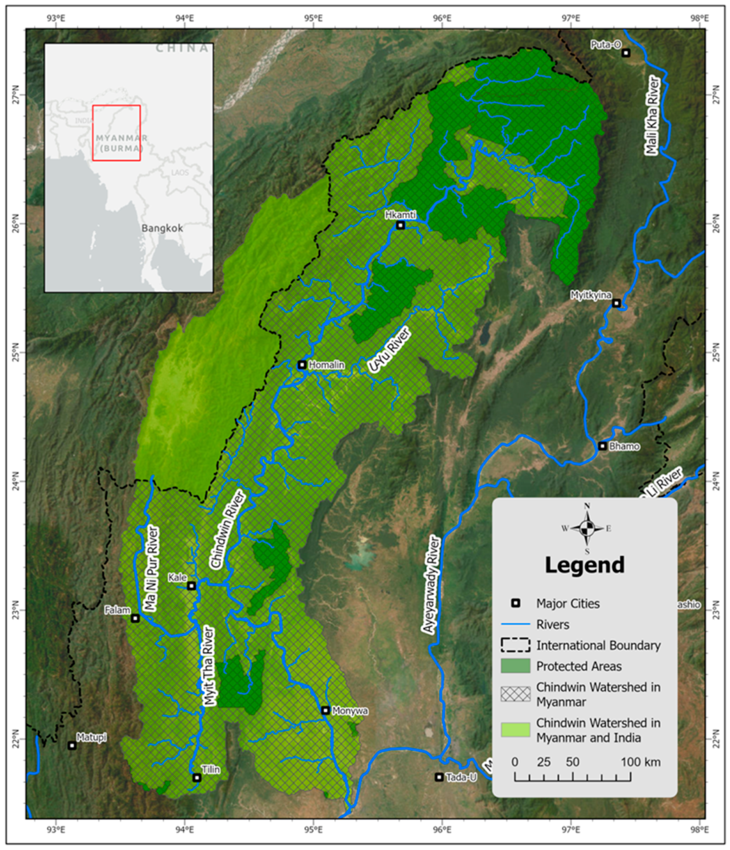
The 114,000-km2 Chindwin River Watershed (CRW; Figure 1) is the largest river watershed of the Ayeyarwady River [33] and has a population of around 6 million people who depend on the river [34]. Originating in the Hukaung Valley in northern Myanmar, the CRW area (93.24° E to 97.30° E and 21.35° N to 27.45° N) is a transboundary river. It shares 16% of its watershed with Manipura State in India [35] and ultimately flows into the Ayeyarwady River. This study, however, only covers areas inside the border of Myanmar.

Figure 1.
Study area map of the Chindwin River Watershed (CRW), Sagaing Region, Myanmar.
The Chindwin River, a major tributary of the Ayeyarwady River in Myanmar, is a vital river ecosystem for several users and consumers, providing various ecological services to people and wildlife in the CRW [34]. The natural biodiversity of the Chindwin watershed makes it one of the most critical hotspots and priority corridors for wild species in the Indo-Burma region. Like other parts of Myanmar, residents of the Chindwin watershed rely heavily on healthy ecosystems for their livelihoods [33]. Currently, 72% of the CRW is covered by forest, a critical energy and construction material source for the watershed’s population [33,34]. Despite the rich natural resources of the CRW [36], only 20% of the watershed is designated as a protected area [35]. This region faces numerous threats due to unmanaged land development, such as forest depletion from mining and logging, construction of hydropower dams, agricultural expansion, and irrigated farming. Additionally, the impacts of climate change further exacerbate these issues [33].
The river has two major tributaries: the Myittha, and U-Yu Rivers. Generally, in almost all watershed regions, the topography is mountainous and forested, except for the southernmost parts, and the elevation ranges from 54 to 3752 m above sea level (a.s.l) [37]. Based on the Köppen–Geiger classification (1991–2020), climate zones in the catchment include monsoon-influenced humid tropical climate (Cwa) and monsoon-influenced temperate climate (Cwb) in the north and tropical savanna climate (As/Aw) in the south (Myanmar—Summary | Climate Change Knowledge Portal [worldbank.org]) [38].
2.2. Conceptual Model
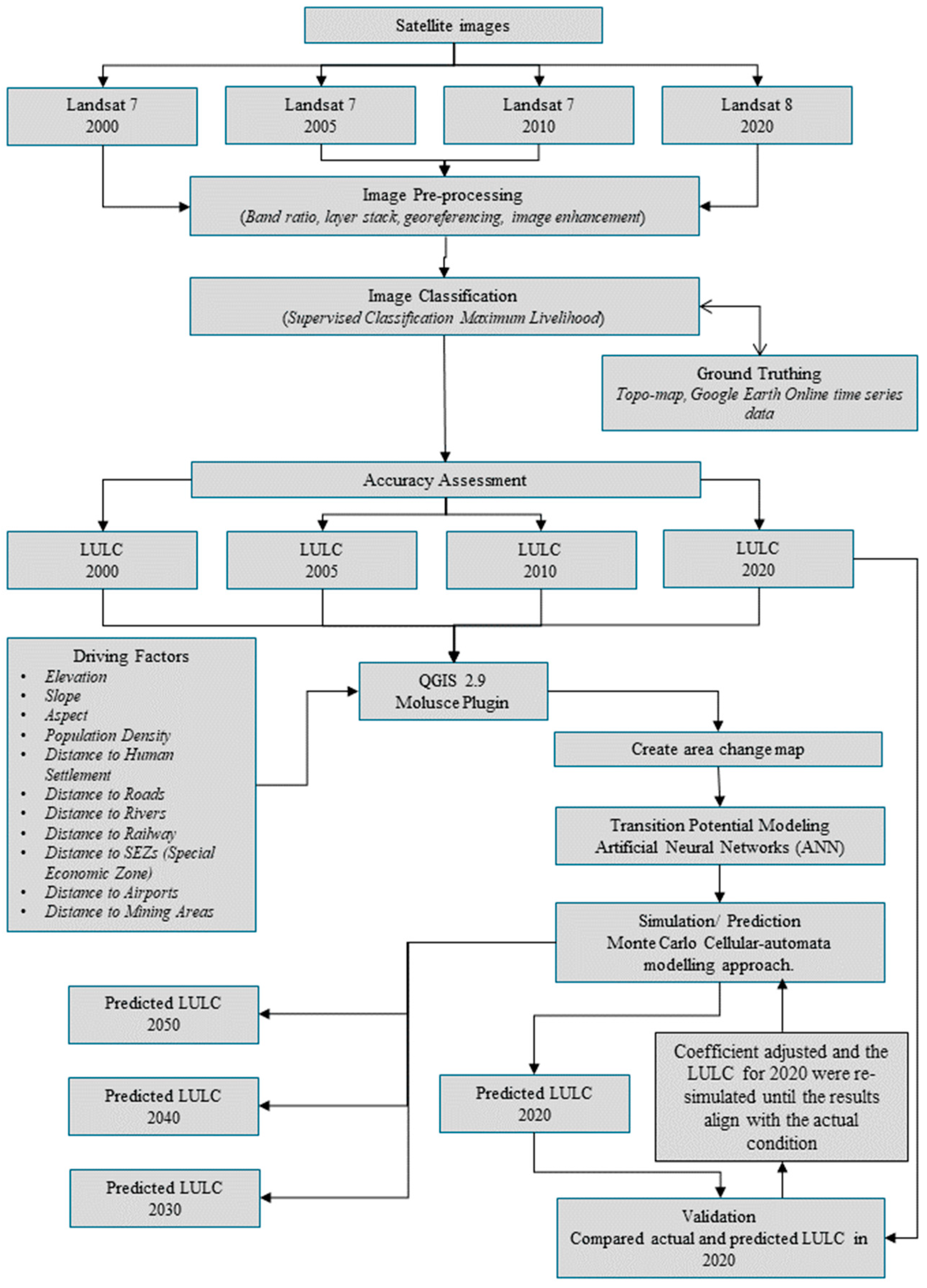
The conceptual model (Figure 2) represents the workflow of LULC classification and future land use prediction. The workflow has three main parts: current LULC classification, LULC prediction, and change.
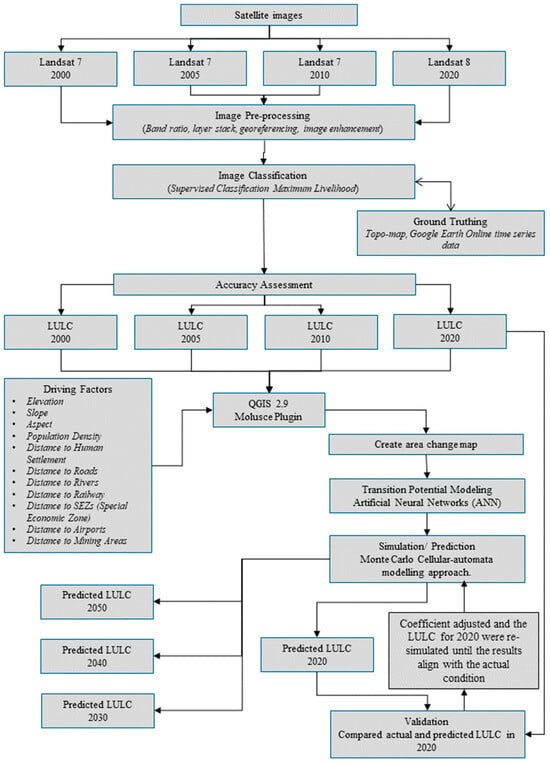
Figure 2.
Workflow for LULC classification and future land used prediction in the Chindwin River Watershed (CRW), Sagaing Region, Myanmar.
2.3. Empirical Methods
2.3.1. LULC Data Acquisition and Preparation
To analyze the land cover changes in the CRW area, we employed remote sensing (RS) technology, geographic information systems (GISs), and various spatial data analysis techniques. The detection of land cover changes from mid-resolution to multi-temporal satellite images such as Landsat, which is one of the most valuable contributions of satellite remote sensing to natural resource management and biodiversity assessments [39].
First and foremost, we acquired satellite imagery from the Landsat dataset developed by the United States Geological Survey (USGS) [40,41]. The data resolution range was 30 × 30 m because this range provided by the Landsat image enables detection of forest and non-forest, as small as 1 ha. However, the CRW area is quite large; therefore, to maintain accuracy and analysis speed, we reduced the resolution to 300 × 300 m. Data were captured by satellite in the same or different years. For example, one season can give minimal cloud coverage, and the same season image can give a stable forest greenness; all images were taken in the open season (December–February) when forest vegetation tends to be lush and cloud cover is low. Therefore, images that contain only less than 2% of cloud coverage were selected and used in our analysis. To decrease the confounding effects of seasonal variations in leaf cover in the mixed deciduous and dry forest within the CRW area, satellite images were chosen for acquisition close to the anniversary date. Although most forest types in the study region are evergreen, a minor portion of dry deciduous forest (teak-bearing forest) can be found in select portions of the river watershed area [42].
For future LULC predictions, we considered DEMs (digital elevation models), slope, population density, distances to airports, human settlement, roads, rivers, and mining as the driving factors of LULC changes in the CRW (Figure A1 and Figure A2). DEM raster files with 30 × 30 m resolution were downloaded from USGS Earth Explorer, and the slope was calculated using the “Slope Tool” with DEM in ArcGIS Pro. Data concerning airports, human settlements, roads, rivers, and distances were downloaded from the Myanmar Information Management Unit (MIMU) [43] in a shape file format and imported into ARC GIS pro software (Version 3.3). The attribute table of the files, as mentioned earlier, was converted to raster format using the Euclidean distance tool available in spatial analysis to obtain the distances from airports, human settlements, roads, rivers, and mining areas. Detailed sources are indicated in Table 1.

Table 1.
Data sources used in the supervised classifications of LULC in Chindwin River Watershed (CRW), Sagaing Region, Myanmar from 2000 to 2020.
2.3.2. LULC Classification
To enhance the classification accuracy, we trained the sample manager using the ArcGIS Pro image classification wizard. High-resolution images for each year were obtained from Google Earth Pro to identify land use categories. Seven categories of land use were identified for classification: human settlement, wetland, bare land, cropland, shrubland, forestland, and water bodies (Appendix A, Table A1). The trained sample was then saved as a shape file for further processing.
For land cover classification, a supervised classification approach using a random tree was employed to generate land use and land cover (LULC) classifications for the Chindwin River Watershed. The random tree algorithm, widely recognized in remote sensing and land cover studies, was selected for its computational efficiency and applicability to multi-temporal satellite data [23]. We calculated the percentage change in LULC from 2010 to 2020 and projected future LULC change scenarios for approximately 2030 and 2050, aligning with climate change scenarios [44].
2.3.3. Accuracy Assessment
The land use categories for accuracy assessment were identified utilizing Google Earth Pro and field inspection methods [45]. Historical images from 2000, 2005, 2015, and 2020 were downloaded with a high-resolution option using Google Earth’s time-lapse feature. We generated 1200 accuracy assessment points as a sample using the ‘create accuracy assessment points’ function in ArcGIS Pro. These data points were then converted to a keyhole markup language (KML) file to visualize the points closer to the location on Google Earth Pro. We used the time slider tap to load the 2000 and 2020 historical maps for accuracy validation. The Kappa coefficient determines the agreement between classification accuracy and reference data [46]. This parameter reflects the difference between the actual agreement and the agreement expected by chance.
2.3.4. LULC Change Analysis Using MLP-ANN (Artificial Neural Network)
Land prediction models such as IDRISI’s CA MARKOV [47], CLUE-S/Dyna-CLUE [48,49], DYNAMICS EGO [50], and the land change modeler [51], forecast when and how frequently LULC changes will occur. These models are particularly useful in determining how previous and future LULC changes may affect soil erosion, especially in farmland [52]. Among the several spatiotemporal dynamic modeling approaches, the cellular automata (CA) model is widely used for land use change analysis [53]. Due to its open structure, the model is widely used for its simplicity, flexibility, and intuitive integration of spatiotemporal elements, making it compatible with other models in anticipating and simulating land use patterns [13].
MOLUSCE (modules of land use change evaluation), a QGIS plugin, is built with the CA model and includes a transition probability matrix that is widely utilized among researchers [54]. This plugin employs four well-known algorithm models: multilayer perceptron artificial neural networks (MLP-ANNs) [55], logistic regression (LR) [56], multi-criteria evaluation (MCE) [57], and weights of evidence (WoE) [58]. Among them, the MLP-ANN model in MOLUSCE is a reliable tool for predicting future LULC that may be utilized in land use planning and management [59]. This model accurately captures nonlinear stochastic processes and generates complex spatial patterns by predicting spatial LULC shifts based on initial conditions, neighboring influences, and transition rules [23].
Therefore, in the CA model, the transition probabilities from the MLP-ANN learning process are employed to generate the LULC changes. Firstly, the model includes the LULC maps for the beginning (2000) and end years (2020). Then, the spatial variable factors, such as human settlement, wetland, bare land, cropland, shrubland, forestland, and water bodies, were imported into the model to obtain a land cover change map from which the changing patterns for the study area between 2005 and 2010 are established (Figure 3). The model calculates the percentage of area changes each year and generates a transition matrix that shows the proportion of pixels shifting from one land use cover to another. Then, future LULC maps are predicted, assuming that existing LULC patterns and dynamics continue. Also, based on the classified raster images of 2000 and 2020, LULC transitions are expected for 2030, 2040, and 2050 [54].
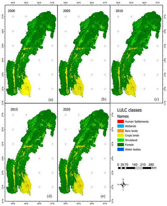
Figure 3.
Supervised classification and LULC classes in the Chindwin River Watershed (CRW), Sagaing Region, Myanmar in (a) 2000, (b) 2005, (c) 2010, (d) 2015, and (e) 2020.
The Kappa coefficient is a widely used metric for generating LULC [60] while validating the accurate and predicted LULC maps (Appendix B, Figure A3) [61]. Validation was carried out between the predicted and actual LULC maps for 2020. The Kappa coefficient is calculated using the expression given below [62]:
where po denotes the proportion of actual agreements and pe denotes the proportion of expected agreements.
3. Results
The Kappa coefficient was 0.76 when excluding the distance to special economic zones (SEZs), railways, and airport variables. The maximum Kappa coefficient of 0.63 is considered a good assessment of accuracy by many researchers [13,52,63,64]. Hence, other variables could strongly influence the prediction of the LULC map of CRW. The LULC maps of 2030, 2040, and 2050 were then predicted using the 2000 and 2020 LULC maps with the same spatial variable combinations (Figure 4).
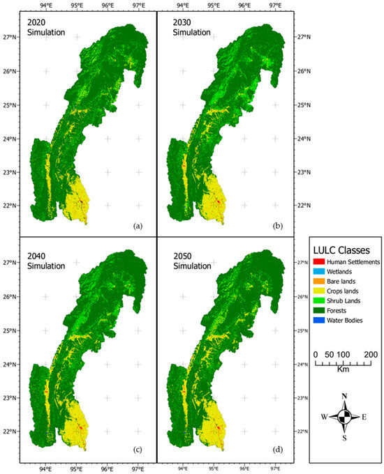
Figure 4.
Predicted LULC maps for the years (a) 2020, (b) 2030, (c) 2040, and (d) 2050 in the Chindwin River Watershed (CRW), Sagaing Region, Myanmar.
The area covered by human settlements increased from 0.22% in 2000 to 0.26% in 2005, subsequently rising to 0.30% by 2010. From 2010 to 2015, there was a slight increase to 0.33%; by 2020, it reached 0.36%. Wetland coverage remained minimal, with only a slight increase from 0.01% in 2005 to 0.02% in 2020. Bare land area decreased from 0.05% in 2000 to 0.03% in 2005, and then experienced significant growth, reaching 0.24% by 2020. On the other hand, cropland coverage expanded from 12.63% in 2000 to 13.52% in 2005. It declined slightly to 13.18% by 2010 but rebounded to 14.01% by 2020. Similarly, the shrubland area increased from 10.37% in 2000 to 11.41% in 2010. It continued to grow, reaching 12.12% by 2020. In contrast, forest land declined from 76.22% in 2000 to 74.62% in 2005. This trend persisted, with a further reduction to 72.71% by 2020. Water bodies remained relatively stable, with minor fluctuations. The coverage was 0.52% in 2000, increased to 0.64% in 2005, and decreased to 0.53% by 2020 (Table 2 and Table 3).
Table 2.
Extent (km2) of current (2000-2020) and predicted (2030-2050) LULCs in Chindwin River Watershed (CRW), Sagaing Region, Myanmar, from 2000 to 2050.
Table 3.
Percentage of LULC in Chindwin River Watershed (CRW), Sagaing Region, Myanmar from 2000 to 2020.
From the perspective of transition probabilities between 2000 and 2020, human settlements had a high probability (0.99) of remaining unchanged. Still, wetlands had a chance of transforming into other types (e.g., shrubland or forestland) as indicated by respective probabilities (e.g., wetlands to shrubland—0.14). The probability of remaining as forestland was 0.90, with a 3% chance of transitioning to cropland and a 6% chance of transitioning to shrubland (Table 4).
Table 4.
Changes over the probability matrix LULC from 2000 to 2020 in the Chindwin River Watershed (CRW), Sagaing Region, Myanmar.
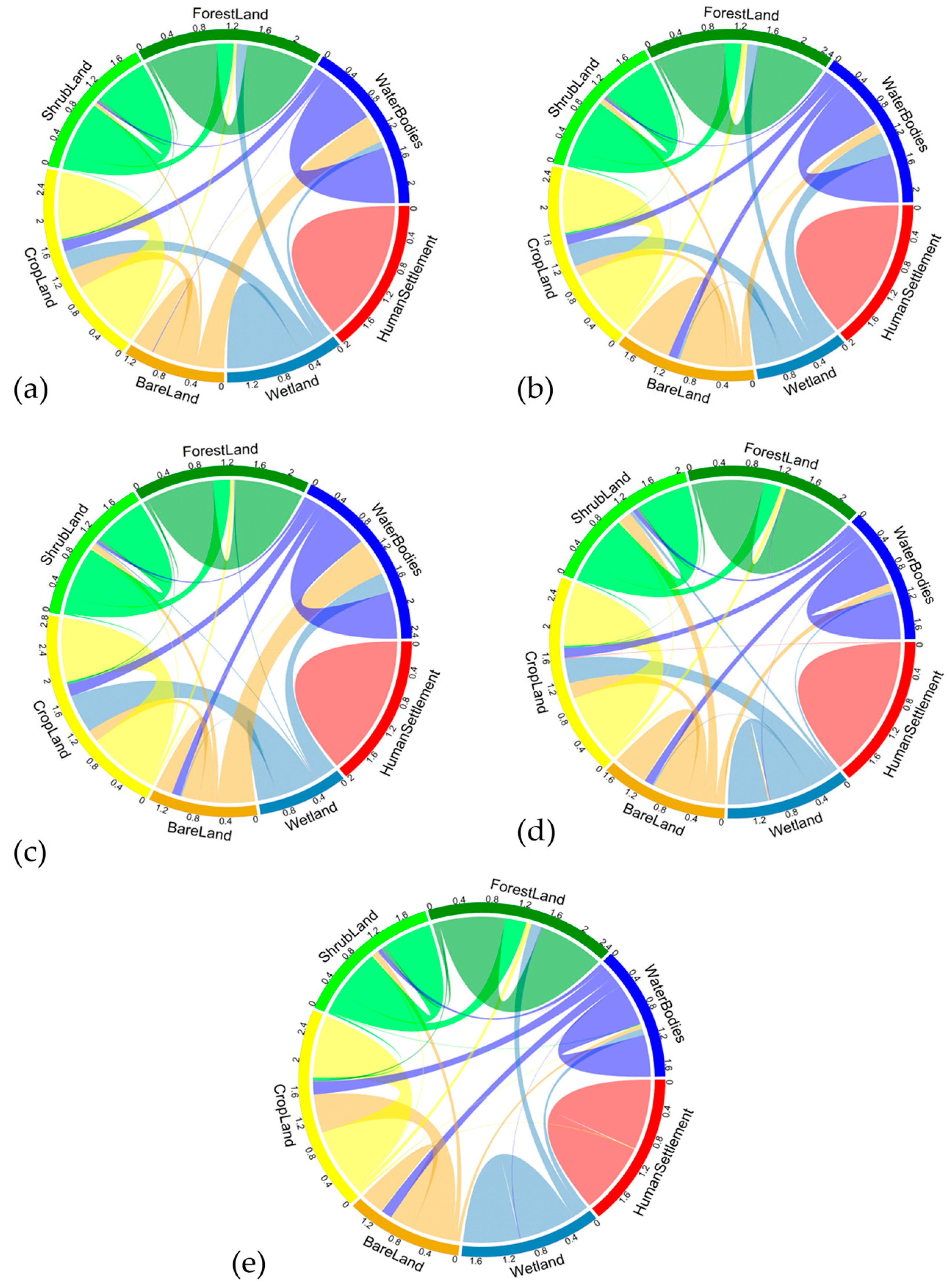
From 2000 to 2020, changes in land use and land cover (LULC) showed that forest land had connections to shrubland, cropland, bare land, wetlands, water bodies, and human settlements (Figure 5). Similarly, waterbodies were connected to almost all other categories except cropland. This implies that waterbodies either increased due to transformations from other land covers or decreased as they transformed into other types. Human settlement had connections with all categories except shrubland, indicating an expansion of human settlement into various land cover types. Wetland connected all categories, indicating loss and gain from/to various land cover types. Wetlands are dynamic and can change due to natural processes or human intervention. Bare land was also connected to all categories except waterbodies. Bare land might be subject to urbanization, agriculture, or other changes (Figure 5).
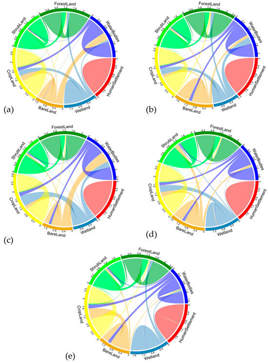
Figure 5.
LULC class transition changes (from–to) (a) 2000–2005, (b) 2005–2010, (c) 2010–15, (d) 2015–2020, (e) 2000–2020 in the Chindwin River Watershed (CRW), Sagaing Region, Myanmar.
As seen through predictions of land use up until 2050, the area covered by human settlements has gradually increased over the years (Figure 4, Table 2). In 2000, it occupied 264 km2; by 2050, it is projected to cover 424 km2 (Table 2). Agricultural lands (croplands) have remained relatively stable regarding total area. They started at 15,204 km2 in 2000 and are projected to cover 18,920 km2 by 2050. Shrublands, characterized by low-growing vegetation, have seen minor fluctuations. They started at 12,490 km2 in 2000 and are projected to cover 12,351 km2 by 2050. Forested areas have remained relatively constant with a slight decrease. In 2000, they covered 91,784 km2; by 2050, they are projected to be 87,837 km2.
4. Discussion
The analysis of land use and land cover (LULC) changes from 2000 to 2020 and projections up to 2050 provide valuable insights into the dynamics of land use and the implications for future land management strategies in the CRW. The increase in human settlements from 0.22% in 2000 to 0.36% in 2020 (64% net increase), with a projected coverage of 424 km2 by 2050, reflects the ongoing urbanization, population growth, and infrastructure development. This expansion signals urbanization, population growth, and infrastructure development. This trend underscores the need for sustainable urban planning to balance development with environmental conservation. One study reported that there was a 1.5% increase in settlement in the Chindwin River Watershed for the period 1999 to 2019 [37]. The difference in estimates between the two studies is due to the former research including all the watershed areas of CRW (including Myanmar and India). In contrast, our research only covered Myanmar areas. Due to the least amount of development in transportation in the CRW field [37], most human settlements increased in the cities surrounding the southern parts and on each side of the major rivers (Figure 3).
The minimal increase in wetland coverage and its high probability of transforming into another type, such as shrubland or forestland, highlight the dynamic nature of wetlands. This could be due to natural processes or human intervention, emphasizing the importance of wetland conservation in maintaining biodiversity and ecosystem services. The significant growth of bare land area from 0.05% in 2000 to 0.24% by 2020 and its projected expansion to 274 km2 by 2050 (a 5-fold increase) could be attributed to deforestation, soil erosion, and land degradation from mining and agricultural expansion. This trend points to the need for effective land management strategies to prevent soil erosion and promote land rehabilitation. The relatively stable cropland coverage and projected increase to 18,920 km2 by 2050 indicate the ongoing demand for agricultural lands. This necessitates sustainable farming practices to ensure food security while minimizing environmental impacts at a watershed scale.
In the CRW, the Sagaing region experienced the highest overall losses in intact forests [40] compared to other regions in Myanmar. The decrease in forested areas from 76.2% in 2000 to 72.7% by 2020 (3% decrease), with a further reduction projected by 2050, raises concerns about deforestation and its implications for biodiversity and climate change. The ~3% decrease in forest area is consistent with the findings [65]. This underscores the importance of forest conservation and sustainable forestry practices. Forest losses can be explained through conversion to (Figure 5, Table 4) shrubland (degraded forest), resulting from overuse of logging, fuel wood consumption, and shifting cultivation [40] and croplands (such as irrigated agricultural lands). Most intact forest areas are in very remote areas (away from major cities) in the CRW. Forest loss hotspots are found at the edges (Figure 4). For example, local hotspots for intact forest loss were identified in Homalin and Hpakant, which are major cities in the CRW, and agree with the gain and loss maps generated in this study [40] (Figure 6).
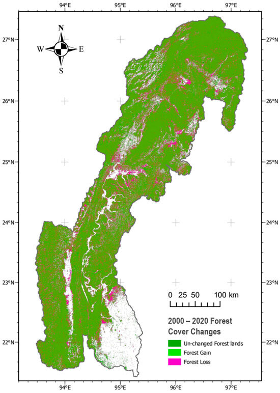
Figure 6.
Forest gain and loss map for Chindwin River Watershed, Sagaing Region, Myanmar.
Illegal, open-pit mining in northern Myanmar, often along streams and rivers, is another major cause of intact forest loss [40]. Although we found mining areas along the Chindwin River in Homalin township, they could not be classified clearly in our methodology because the reflectance from the non-irrigated agricultural land (bare land without vegetation) was like that from open-pit mining areas. Extensive field surveys and high-resolution satellite imagery would be needed to differentiate between them.
The data (Table 2 and Figure 5) provide insights into dynamic changes occurring across various land use and land cover (LULC) categories from 2000 to 2020 and predicted to 2030, 2040, and 2050. A notable trend was observed in human settlements, which expanded significantly, while wetlands experienced growth with minor fluctuations, indicating efforts toward conservation or natural expansion due to climatic factors. Bare land, devoid of significant vegetation or structures, has shown substantial variability. From an initial 54 km2 in 2000, it will expand significantly to 274 km2 by 2050. Deforestation, soil erosion, and land degradation may contribute to these changes. Croplands exhibited consistent growth, reflecting increased agricultural activities, possibly due to growing population demands. On the other hand, forest lands depicted a gradual decline until about four decades post-millennium before showing signs of recovery; this underscores concerns related to deforestation and highlights potential reforestation or natural regeneration events occurring later [33].
Regarding the gain and loss of forest extent in the CRW (Figure 6), unchanged forest lands (stable forest extent) are the predominant green areas, signifying regions where the forest cover has remained intact over the two decades. These unchanged forest lands are critical for biodiversity, carbon sequestration, and ecosystem services. They represent stable ecosystems that have not experienced significant disturbances or deforestation [33]. Pockets of pink dispersed throughout the map denote areas of forest loss. These regions have experienced changes such as deforestation, logging, or natural calamities. Reducing forest cover may adversely affect local climate, wildlife habitats, and soil stability. Minimal blue patches symbolize areas of new forest growth or reforestation efforts during the specified period. These gains could result from afforestation projects, reforestation initiatives, or natural regeneration. Forest gain is crucial for restoring ecosystem functions, enhancing landscape connectivity, and mitigating climate change.
The spatial distribution of forest gain and loss forms distinct hotspots. These localized patterns highlight areas where conservation efforts have succeeded, or deforestation pressures are particularly intense. Understanding these regional dynamics is essential for targeted interventions and sustainable forest management [66]. In summary, the gain and loss of forest extent underscores the dynamic nature of forest landscape in the CRW. It emphasizes the need for strategic conservation, afforestation, and monitoring efforts to balance forest loss with gain. Sustainable land use practices are crucial to maintaining healthy ecosystems and supporting local communities [33].
Moreover, this study emphasizes that changes in watershed land use threaten watershed processes, including ecosystem services like habitat, connectivity, and livelihoods of local people. However, extensive threats posed by unmanaged development pose risks, especially from mining, logging, and hydropower expansion. Integrated conservation strategies are urgently required to safeguard ecosystems that local communities depend upon. Adaptive habitat management and species conservation action plans can help mitigate those risks. The World Bank has recommended the main elements for an effective policy and regulatory framework on land in Myanmar, including protecting customary users’ tenure rights and promoting diverse agricultural practices while securing nature and wildlands [67].
By linking the related existing land policies and regulations with the study’s emphasis on habitat connectivity and wildlife corridors, it becomes clear that a multi-stakeholder approach is necessary. This approach should combine legal reform, community involvement, and sustainable land management practices to preserve tropical ecosystems and the wildlife corridors within the CRW that are vital for biodiversity conservation.
5. Conclusions
This research underscores the potential impact of anthropogenic land use activities on the geographical distribution of ecological services and wildlife habitats in Myanmar’s Chindwin River Watershed (CRW). This study highlights the urgent need for adaptive management strategies such as enhancing ecological zone prioritization, flexible zoning regulations for urban development, and adopting an adaptative governance system that considers land use changes to safeguard these concerns and minimize habitat loss. The analysis of land use and land cover (LULC) changes from 2000 to 2020 reveals significant shifts in various land categories, most notably the expansion of human settlements and the decline of forest land. These changes, coupled with the predicted future land use until 2050, indicate an escalating threat to the biodiversity of the CRW. Moreover, the study’s findings emphasize the critical role of the CRW in maintaining key biodiversity areas for endemic and endangered species and providing essential ecosystem services for local communities. However, the future of the CRW is threatened by extensive risk of land use changes.
In conclusion, this study underscores the urgent need for comprehensive and integrated conservation strategies that address the impacts of land use alterations. Such strategies are crucial for preserving the rich biodiversity of the CRW and ensuring the sustainability of the ecosystems upon which local communities heavily rely. The insights derived from this study could significantly contribute to formulating such strategies and action plans, thereby playing a pivotal role in species conservation in the region.
Author Contributions
Conceptualization, T.T.B. and T.O.R.; methodology, T.T.B. and T.O.R.; software, T.T.B. and T.O.R.; validation, T.T.B. and T.O.R.; formal analysis, T.T.B. and T.O.R.; investigation, T.T.B. and T.O.R.; resources, T.O.R.; data curation, T.T.B.; writing—original draft preparation, T.T.B. and T.O.R.; writing—review and editing, T.T.B. and T.O.R.; visualization, T.T.B.; supervision, T.O.R.; project administration, T.T.B. and T.O.R.; funding acquisition, T.T.B. and T.O.R. All authors have read and agreed to the published version of the manuscript.
Funding
This research received no external funding.
Data Availability Statement
The data that support and underlie this study are from publicly available sources that are openly accessible via these in-text data citation references: USGS (2023), MIMU (2023), and NextGIS (2017).
Conflicts of Interest
The authors declare no conflicts of interest.
Appendix A
Table A1.
LULC category description and training sample at Google Earth Pro points were used in supervised classifications of LULC in the Chindwin River Watershed (CRW), Sagaing Region, Myanmar from 2000 to 2020.
Table A1.
LULC category description and training sample at Google Earth Pro points were used in supervised classifications of LULC in the Chindwin River Watershed (CRW), Sagaing Region, Myanmar from 2000 to 2020.
| LULC Category | Description | Training Sample |
|---|---|---|
| Forest | Any significant clustering of tall (~15 feet or higher) dense vegetation, typically with a closed or dense canopy; examples: wooded vegetation, clusters of dense tall vegetation within savannas, plantations, swamp or mangroves (dense/tall vegetation with ephemeral water or canopy too thick to detect water underneath). |  |
| Crop lands | Human-planted/plotted cereals, grasses, and crops not at tree height; examples: corn, wheat, soy, and fallow plots of structured land. |  |
| Human settlement | Human-made structures; large homogenous impervious surfaces, including parking structures, office buildings, and residential housing; examples: houses, dense villages/towns/cities, paved roads, asphalt. |  |
| Bare lands | Areas of rock or soil with very little to no vegetation for the entire year; large areas of sand and deserts with no to little vegetation; examples: exposed rock or soil, deserts, sand dunes, dried lake beds, and mines. |  |
| Shrub lands | Open areas covered in homogenous grasses with little to no taller vegetation; wild cereals and grasses with no obvious human plotting (i.e., not a plotted field); examples: natural meadows and fields with little to no tree cover, open savanna with few to no trees, parks/golf courses/lawns, pastures. A mix of small clusters of plants or single plants dispersed on a landscape that shows exposed soil or rock; scrub-filled clearings within dense forests that are clearly not taller than trees; examples: moderate to little cover of bushes, shrubs, tufts of grass, savannas with very little grasses, trees, or other plants. |  |
| Water | Areas where water was predominantly present throughout the year; may not cover areas with sporadic or ephemeral water; contains little to no vegetation, no rock outcrop nor built-up features like docks; examples: rivers, ponds, lakes, oceans, and flooded salt plains. |  |
| Wetland | Wetlands are areas where water covers the soil or is present either at or near the surface of the soil all year or for varying periods of time during the year, including during the growing season. |  |
Table A2.
Accuracy assessment evaluation in different classified images of different time scales while calculating current and historical LULC classification.
Table A2.
Accuracy assessment evaluation in different classified images of different time scales while calculating current and historical LULC classification.
| No. | Classes | 2000 | 2005 | 2010 | 2015 | 2020 | |||||
|---|---|---|---|---|---|---|---|---|---|---|---|
| User’s accuracy (%) | Producer’s accuracy (%) | User’s accuracy (%) | Producer’s accuracy (%) | User’s accuracy (%) | Producer’s accuracy (%) | User’s accuracy (%) | Producer’s accuracy (%) | User’s accuracy (%) | Producer’s accuracy (%) | ||
| 1 | Human Settlement | 95.28 | 96.84 | 96.89 | 97.33 | 76.55 | 89 | 99.33 | 100 | 87.94 | 92.82 |
| 2 | Wetlands | 98.97 | 99.84 | 92.96 | 93.43 | 70 | 75.43 | 95.03 | 96 | 98.54 | 99.2 |
| 3 | Bare lands | 92.52 | 94.6 | 97.94 | 98 | 63.01 | 63.85 | 98.17 | 99.54 | 89.74 | 90.2 |
| 4 | Crop lands | 76.75 | 92.5 | 93.24 | 95.46 | 80.98 | 81.76 | 98.47 | 99.36 | 94.33 | 95.64 |
| 5 | Shrubland | 85.93 | 90.5 | 96.15 | 97.89 | 79.1 | 83 | 97.86 | 98.43 | 90.02 | 95.44 |
| 6 | Forests | 98.76 | 100 | 97.24 | 97.68 | 74.04 | 76.89 | 98.67 | 99.12 | 92.72 | 93.43 |
| 7 | Water bodies | 99.54 | 100 | 100 | 100 | 89.97 | 90.45 | 99.29 | 100 | 100 | 100 |
| 8 | Overall accuracy | 92.54 | 96.35 | 76.24 | 98.12 | 93.33 | |||||
| 9 | Kappa Coefficient | 0.97 | 0.96 | 0.73 | 0.95 | 0.93 | |||||
Table A3.
Kappa index of the model validation (simulated 2020 LULC with reference 2020) while predicting the future LULC in the Chindwin River Basin.
Table A3.
Kappa index of the model validation (simulated 2020 LULC with reference 2020) while predicting the future LULC in the Chindwin River Basin.
| Parameter | Value (%) |
|---|---|
| Kappa (histogram) | 0.94 |
| Kappa (overall) | 0.63 |
| Kappa (location) | 0.70 |
| % of correctness | 76.00 |
Appendix B
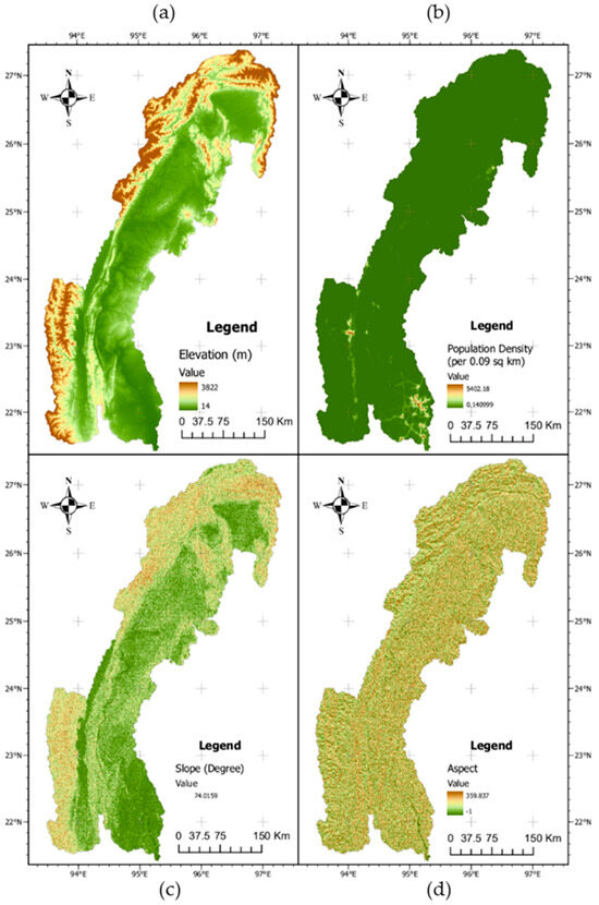
Figure A1.
Explanatory maps: (a) DEM (digital elevation model), (b) population density, (c) slope, and (d) aspect in the Chindwin River Watershed (CRW), Sagaing Region, Myanmar.
Figure A1.
Explanatory maps: (a) DEM (digital elevation model), (b) population density, (c) slope, and (d) aspect in the Chindwin River Watershed (CRW), Sagaing Region, Myanmar.

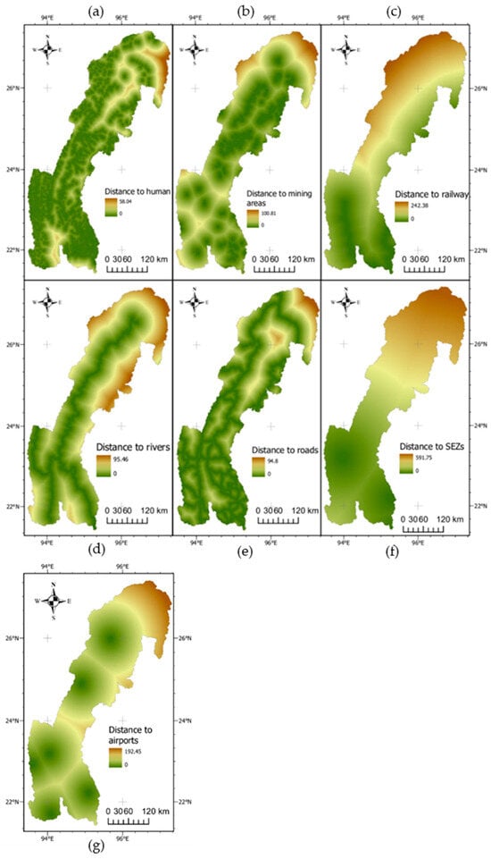
Figure A2.
Explanatory maps: distances to (a) human settlement, (b) mining area, (c) railway, (d) rivers, (e) roads, (f) SEZs (Special Economic Zones), and (g) airports in the Chindwin River Watershed (CRW), Sagaing Region, Myanmar.
Figure A2.
Explanatory maps: distances to (a) human settlement, (b) mining area, (c) railway, (d) rivers, (e) roads, (f) SEZs (Special Economic Zones), and (g) airports in the Chindwin River Watershed (CRW), Sagaing Region, Myanmar.
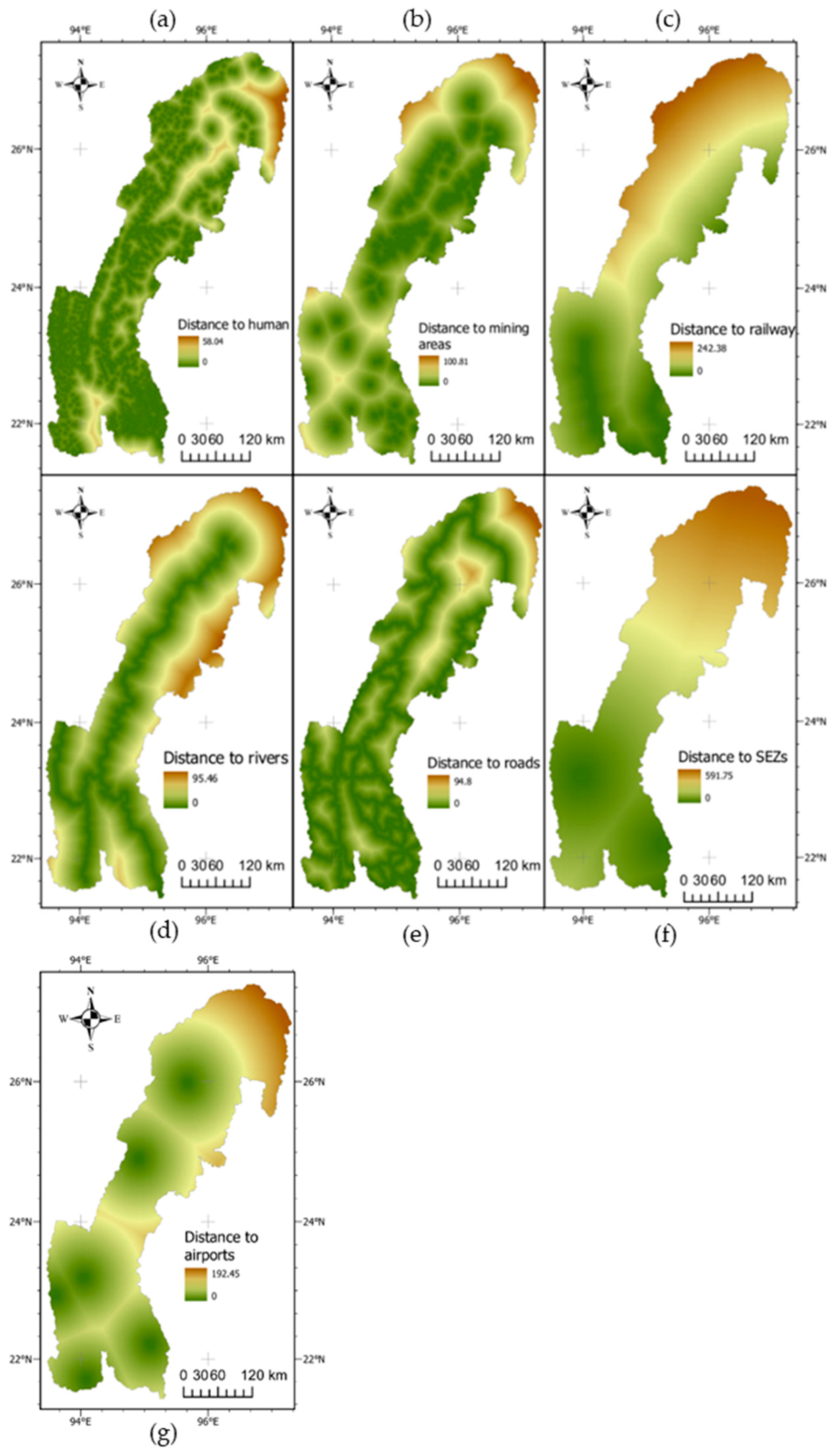
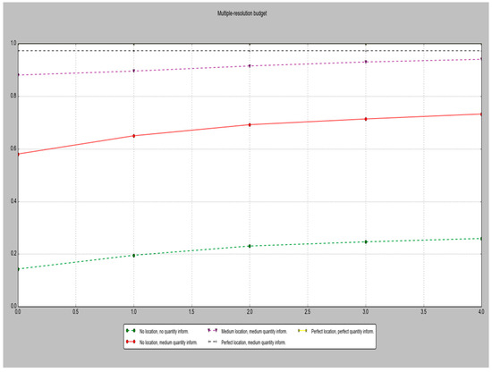
Figure A3.
Validation graph between the observed 2020 and predicted 2020 LULC map for the Chindwin River Watershed (CRW), Sagaing Region, Myanmar.
Figure A3.
Validation graph between the observed 2020 and predicted 2020 LULC map for the Chindwin River Watershed (CRW), Sagaing Region, Myanmar.
References
- Talib, A.; Randhir, T.O. Long-Term Effects of Land-Use Change on Water Resources in Urbanizing Watersheds. PLOS Water 2023, 2, e0000083. [Google Scholar] [CrossRef]
- Newbold, T. Future Effects of Climate and Land-Use Change on Terrestrial Vertebrate Community Diversity under Different Scenarios. Proc. R. Soc. B. 2018, 285, 20180792. [Google Scholar] [CrossRef] [PubMed]
- Sieber, A.; Uvarov, N.V.; Baskin, L.M.; Radeloff, V.C.; Bateman, B.L.; Pankov, A.B.; Kuemmerle, T. Post-Soviet Land-Use Change Effects on Large Mammals’ Habitat in European Russia. Biol. Conserv. 2015, 191, 567–576. [Google Scholar] [CrossRef]
- Foley, J.A.; DeFries, R.; Asner, G.P.; Barford, C.; Bonan, G.; Carpenter, S.R.; Chapin, F.S.; Coe, M.T.; Daily, G.C.; Gibbs, H.K.; et al. Global Consequences of Land Use. Science 2005, 309, 570–574. [Google Scholar] [CrossRef] [PubMed]
- Turner, B.L.; Lambin, E.F.; Reenberg, A. The Emergence of Land Change Science for Global Environmental Change and Sustainability. Proc. Natl. Acad. Sci. USA 2007, 104, 20666–20671. [Google Scholar] [CrossRef] [PubMed]
- Pekin, B.K.; Pijanowski, B.C. Global Land Use Intensity and the Endangerment Status of Mammal Species. Diversity Distrib. 2012, 18, 909–918. [Google Scholar] [CrossRef]
- Randhir, T. Watershed-scale Effects of Urbanization on Sediment Export: Assessment and Policy. Water Resour. Res. 2003, 39, 2002WR001913. [Google Scholar] [CrossRef]
- Mamba, H.S.; Randhir, T.O. Exploring Temperature and Precipitation Changes under Future Climate Change Scenarios for Black and White Rhinoceros Populations in Southern Africa. Biodiversity 2024, 25, 52–64. [Google Scholar] [CrossRef]
- Nampindo, S.; Randhir, T.O. Dynamic Modeling of African Elephant Populations under Changing Climate and Habitat Loss across the Greater Virunga Landscape. PLoS Sustain. Transform. 2024, 3, e0000094. [Google Scholar] [CrossRef]
- Thuiller, W.; Broennimann, O.; Hughes, G.; Alkemade, J.R.M.; Midgley, G.F.; Corsi, F. Vulnerability of African Mammals to Anthropogenic Climate Change under Conservative Land Transformation Assumptions: VULNERABILITY OF AFRICAN MAMMALS TO ANTHROPOGENIC CC. Glob. Chang. Biol. 2006, 12, 424–440. [Google Scholar] [CrossRef]
- Parker, D.C.; Manson, S.M.; Janssen, M.A.; Hoffmann, M.J.; Deadman, P. Multi-Agent Systems for the Simulation of Land-Use and Land-Cover Change: A Review. Ann. Assoc. Am. Geogr. 2003, 93, 314–337. [Google Scholar] [CrossRef]
- Verburg, P.H.; Schot, P.P.; Dijst, M.J.; Veldkamp, A. Land Use Change Modelling: Current Practice and Research Priorities. GeoJournal 2004, 61, 309–324. [Google Scholar] [CrossRef]
- Alam, N.; Saha, S.; Gupta, S.; Chakraborty, S. Prediction Modelling of Riverine Landscape Dynamics in the Context of Sustainable Management of Floodplain: A Geospatial Approach. Ann. GIS 2021, 27, 299–314. [Google Scholar] [CrossRef]
- Muche, M.; Yemata, G.; Molla, E.; Adnew, W.; Muasya, A.M. Land Use and Land Cover Changes and Their Impact on Ecosystem Service Values in the North-Eastern Highlands of Ethiopia. PLoS ONE 2023, 18, e0289962. [Google Scholar] [CrossRef] [PubMed]
- Astuti, I.S.; Sahoo, K.; Milewski, A.; Mishra, D.R. Impact of Land Use Land Cover (LULC) Change on Surface Runoff in an Increasingly Urbanized Tropical Watershed. Water Resour Manag. 2019, 33, 4087–4103. [Google Scholar] [CrossRef]
- Esfandeh, S.; Danehkar, A.; Salmanmahiny, A.; Sadeghi, S.M.M.; Marcu, M.V. Climate Change Risk of Urban Growth and Land Use/Land Cover Conversion: An In-Depth Review of the Recent Research in Iran. Sustainability 2021, 14, 338. [Google Scholar] [CrossRef]
- Yao, Y.; Yan, X.; Luo, P.; Liang, Y.; Ren, S.; Hu, Y.; Han, J.; Guan, Q. Classifying Land-Use Patterns by Integrating Time-Series Electricity Data and High-Spatial Resolution Remote Sensing Imagery. Int. J. Appl. Earth Obs. Geoinf. 2022, 106, 102664. [Google Scholar] [CrossRef]
- Souza, J.M.D.; Morgado, P.; Costa, E.M.D.; Vianna, L.F.D.N. Modeling of Land Use and Land Cover (LULC) Change Based on Artificial Neural Networks for the Chapecó River Ecological Corridor, Santa Catarina/Brazil. Sustainability 2022, 14, 4038. [Google Scholar] [CrossRef]
- Liu, B.; Song, W.; Meng, Z.; Liu, X. Review of Land Use Change Detection—A Method Combining Machine Learning and Bibliometric Analysis. Land 2023, 12, 1050. [Google Scholar] [CrossRef]
- M, A.; Ahmed, S.A.; N, H. Land Use and Land Cover Classification Using Machine Learning Algorithms in Google Earth Engine. Earth Sci. Inform. 2023, 16, 3057–3073. [Google Scholar] [CrossRef]
- Avci, C.; Budak, M.; Yağmur, N.; Balçik, F. Comparison between Random Forest and Support Vector Machine Algorithms for LULC Classification. Int. J. Eng. Geosci. 2023, 8, 1–10. [Google Scholar] [CrossRef]
- Breiman, L. Random Forests. Mach. Learn. 2001, 45, 5–32. [Google Scholar] [CrossRef]
- Prasad, A.M.; Iverson, L.R.; Liaw, A. Newer Classification and Regression Tree Techniques: Bagging and Random Forests for Ecological Prediction. Ecosystems 2006, 9, 181–199. [Google Scholar] [CrossRef]
- Lek, S.; Guégan, J.F. Artificial Neural Networks as a Tool in Ecological Modelling, an Introduction, Ecological Modelling. Ecol. Model. 1999, 120, 65–73. [Google Scholar] [CrossRef]
- Chaturvedi, V.; De Vries, W.T. Machine Learning Algorithms for Urban Land Use Planning: A Review. Urban Sci. 2021, 5, 68. [Google Scholar] [CrossRef]
- Fontana, A.G.; Nascimento, V.F.; Ometto, J.P.; Do Amaral, F.H.F. Analysis of Past and Future Urban Growth on a Regional Scale Using Remote Sensing and Machine Learning. Front. Remote Sens. 2023, 4, 1123254. [Google Scholar] [CrossRef]
- Tanaka, Y.; Minggat, E.; Roseli, W. The Impact of Tropical Land-Use Change on Downstream Riverine and Estuarine Water Properties and Biogeochemical Cycles: A Review. Ecol. Process 2021, 10, 40. [Google Scholar] [CrossRef]
- Chen, C.-F.; Son, N.-T.; Chang, N.-B.; Chen, C.-R.; Chang, L.-Y.; Valdez, M.; Centeno, G.; Thompson, C.; Aceituno, J. Multi-Decadal Mangrove Forest Change Detection and Prediction in Honduras, Central America, with Landsat Imagery and a Markov Chain Model. Remote Sens. 2013, 5, 6408–6426. [Google Scholar] [CrossRef]
- Richards, D.R.; Friess, D.A. Rates and Drivers of Mangrove Deforestation in Southeast Asia, 2000–2012. Proc. Natl. Acad. Sci. USA 2016, 113, 344–349. [Google Scholar] [CrossRef]
- Gameiro, S.; Nascimento, V.; Facco, D.; Sfredo, G.; Ometto, J. Multitemporal Spatial Analysis of Land Use and Land Cover Changes in the Lower Jaguaribe Hydrographic Sub-Basin, Ceará, Northeast Brazil. Land 2022, 11, 103. [Google Scholar] [CrossRef]
- Asmara, B.; Randhir, T.O. Modeling the Impacts of Oil Palm Plantations on Water Quantity and Quality in the Kais River Watershed of Indonesia. Sci. Total Environ. 2024, 928, 172456. [Google Scholar] [CrossRef]
- Diffenbaugh, N.S.; Field, C.B. Changes in Ecologically Critical Terrestrial Climate Conditions. Science 2013, 341, 486–492. [Google Scholar] [CrossRef] [PubMed]
- Shrestha, M.; Piman, T.; Grünbühel, C. Prioritizing Key Biodiversity Areas for Conservation Based on Threats and Ecosystem Services Using Participatory and GIS-Based Modeling in Chindwin River Basin, Myanmar. Ecosyst. Serv. 2021, 48, 101244. [Google Scholar] [CrossRef]
- Krittasudthacheewa, C.; Maung, W.; Lebel, L.; Danial, R.; Hongsathavij, V. (Eds.) Chindwin Futures: Natural Resources, Livelihoods, Institutions, and Climate Change in Myanmar’s Chindwin River Basin; Strategic Information and Research Development Centre and Stockholm Environment Institute (SEI) Asia Centre: Petaling Jaya, Malaysia, 2021; ISBN 9789672464310. [Google Scholar]
- IFC—International Finance Corporation Baseline Assessment Report Hydropower: Strategic Environmental Assessment of the Hydropower Sector in Myanmar. 2017, pp. 1–127. Available online: https://www.google.com.hk/url?sa=t&source=web&rct=j&opi=89978449&url=https://www.ifc.org/content/dam/ifc/doc/mgrt/chapter-2-sea-baseline-assessment-hydropower.pdf&ved=2ahUKEwiR4ofq6cuHAxXGga8BHQeQJ30QFnoECBYQAQ&usg=AOvVaw0F_jjMil1yY5pexlVjh1X4 (accessed on 5 July 2024).
- Grill, G.; Lehner, B.; Thieme, M.; Geenen, B.; Tickner, D.; Antonelli, F.; Babu, S.; Borrelli, P.; Cheng, L.; Crochetiere, H.; et al. Mapping the World’s Free-Flowing Rivers. Nature 2019, 569, 215–221. [Google Scholar] [CrossRef] [PubMed]
- McGinn, A.J.; Wagner, P.D.; Htike, H.; Kyu, K.K.; Fohrer, N. Twenty Years of Change: Land and Water Resources in the Chindwin Catchment, Myanmar between 1999 and 2019. Sci. Total Environ. 2021, 798, 148766. [Google Scholar] [CrossRef]
- World Bank Climate Change Knowledge Portal. Available online: https://climateknowledgeportal.worldbank.org/ (accessed on 18 December 2023).
- Turner, W.; Spector, S.; Gardiner, N.; Fladeland, M.; Sterling, E.; Steininger, M. Remote Sensing for Biodiversity Science and Conservation. Trends Ecol. Evol. 2003, 18, 306–314. [Google Scholar] [CrossRef]
- Bhagwat, T.; Hess, A.; Horning, N.; Khaing, T.; Thein, Z.M.; Aung, K.M.; Aung, K.H.; Phyo, P.; Tun, Y.L.; Oo, A.H.; et al. Losing a Jewel—Rapid Declines in Myanmar’s Intact Forests from 2002–2014. PLoS ONE 2017, 12, e0176364. [Google Scholar] [CrossRef]
- Landsat-7 Image Courtesy of the U.S. Geological Survey. Available online: https://www.usgs.gov/landsat-missions/landsat-7 (accessed on 15 September 2023).
- Htike, M.H.; Naing, H.; Tizard, R. Hoolock Gibbon Survey and Monitoring in Htamanthi Wildlife Sanctuary, Sagaing Region; WCS Myanmar Program: Yangon, Myanmar, 2019. [Google Scholar]
- Myanmar Information Management Unit (MIMU). 2023. Available online: https://themimu.info/baseline-datasets. (accessed on 3 December 2023).
- Intergovernmental Panel On Climate Change. Climate Change and Land: IPCC Special Report on Climate Change, Desertification, Land Degradation, Sustainable Land Management, Food Security, and Greenhouse Gas Fluxes in Terrestrial Ecosystems, 1st ed.; Cambridge University Press: Cambridge, CA, USA, 2022; ISBN 978-1-00-915798-8.
- Vijitharan, S.; Sasaki, N.; Venkatappa, M.; Tripathi, N.K.; Abe, I.; Tsusaka, T.W. Assessment of Forest Cover Changes in Vavuniya District, Sri Lanka: Implications for the Establishment of Subnational Forest Reference Emission Level. Land 2022, 11, 1061. [Google Scholar] [CrossRef]
- Pontius, R.G.; Millones, M. Death to Kappa: Birth of Quantity Disagreement and Allocation Disagreement for Accuracy Assessment. Int. J. Remote Sens. 2011, 32, 4407–4429. [Google Scholar] [CrossRef]
- Paegelow, M.; Olmedo, M.T.C. Possibilities and Limits of Prospective GIS Land Cover Modelling—A Compared Case Study: Garrotxes (France) and Alta Alpujarra Granadina (Spain). Int. J. Geogr. Inf. Sci. 2005, 19, 697–722. [Google Scholar] [CrossRef]
- Verburg, P.H.; Soepboer, W.; Veldkamp, A.; Limpiada, R.; Espaldon, V.; Mastura, S.S.A. Modeling the Spatial Dynamics of Regional Land Use: The CLUE-S Model. Environ. Manag. 2002, 30, 391–405. [Google Scholar] [CrossRef] [PubMed]
- Verburg, P.H.; Overmars, K.P. Combining Top-down and Bottom-up Dynamics in Land Use Modeling: Exploring the Future of Abandoned Farmlands in Europe with the Dyna-CLUE Model. Landscape Ecol. 2009, 24, 1167–1181. [Google Scholar] [CrossRef]
- Soares-Filho, B.S.; Coutinho Cerqueira, G.; Lopes Pennachin, C. Dinamica—A Stochastic Cellular Automata Model Designed to Simulate the Landscape Dynamics in an Amazonian Colonization Frontier. Ecol. Model. 2002, 154, 217–235. [Google Scholar] [CrossRef]
- Khoi, D.D.; Murayama, Y. Forecasting Areas Vulnerable to Forest Conversion in the Tam Dao National Park Region, Vietnam. Remote Sens. 2010, 2, 1249–1272. [Google Scholar] [CrossRef]
- Perović, V.; Jakšić, D.; Jaramaz, D.; Koković, N.; Čakmak, D.; Mitrović, M.; Pavlović, P. Spatio-Temporal Analysis of Land Use/Land Cover Change and Its Effects on Soil Erosion (Case Study in the Oplenac Wine-Producing Area, Serbia). Environ. Monit. Assess 2018, 190, 675. [Google Scholar] [CrossRef] [PubMed]
- Guan, D.; Gao, W.; Watari, K.; Fukahori, H. Land Use Change of Kitakyushu Based on Landscape Ecology and Markov Model. J. Geogr. Sci. 2008, 18, 455–468. [Google Scholar] [CrossRef]
- NextGIS MOLUSCE-Quick and Convenient Analysis of Land Cover Changes. MOLUSCE-Quick and Convenient Analysis of LandCoverChanges. 2017. Available online: https://nextgis.com/blog/molusce/ (accessed on 15 September 2023).
- Atkinson, P.M.; Tatnall, A.R.L. Introduction Neural Networks in Remote Sensing. Int. J. Remote Sens. 1997, 18, 699–709. [Google Scholar] [CrossRef]
- Buya, S.; Tongkumchum, P.; Owusu, B.E. Modelling of Land-Use Change in Thailand Using Binary Logistic Regression and Multinomial Logistic Regression. Arab. J. Geosci. 2020, 13, 437. [Google Scholar] [CrossRef]
- Malczewski, J.; Rinner, C. Multicriteria Decision Analysis in Geographic Information Science; Advances in Geographic Information Science; Springer: Berlin/Heidelberg, Germany, 2015; ISBN 978-3-540-74756-7. [Google Scholar]
- Khan, M.; Tahir, A.A.; Ullah, S.; Khan, R.; Ahmad, K.; Shahid, S.U.; Nazir, A. Trends and Projections of Land Use Land Cover and Land Surface Temperature Using an Integrated Weighted Evidence-Cellular Automata (WE-CA) Model. Environ. Monit. Assess 2022, 194, 120. [Google Scholar] [CrossRef]
- Saputra, M.H.; Lee, H.S. Prediction of Land Use and Land Cover Changes for North Sumatra, Indonesia, Using an Artificial-Neural-Network-Based Cellular Automaton. Sustainability 2019, 11, 3024. [Google Scholar] [CrossRef]
- Congalton, R.G.; Green, K. Assessing the Accuracy of Remotely Sensed Data: Principles and Practices, 3rd ed.; CRC Press: Boca Raton, FL, USA, 2019; ISBN 978-0-429-05272-9. [Google Scholar]
- Arumugam, T.; Yadav, R.L.; Kinattinkara, S. Assessment and Predicting of LULC by Kappa Analysis and CA Markov Model Using RS and GIS Techniques in Udham Singh Nagar District, India. Res. Square, 2021; 3, 1–24. [Google Scholar]
- Kamaraj, M.; Rangarajan, S. Predicting the Future Land Use and Land Cover Changes for Bhavani Basin, Tamil Nadu, India, Using QGIS MOLUSCE Plugin. Environ. Sci. Pollut. Res. 2022, 29, 86337–86348. [Google Scholar] [CrossRef] [PubMed]
- Aneesha Satya, B.; Shashi, M.; Deva, P. Future Land Use Land Cover Scenario Simulation Using Open Source GIS for the City of Warangal, Telangana, India. Appl. Geomat. 2020, 12, 281–290. [Google Scholar] [CrossRef]
- Rahman, M.T.U.; Tabassum, F.; Rasheduzzaman, M.; Saba, H.; Sarkar, L.; Ferdous, J.; Uddin, S.Z.; Zahedul Islam, A.Z.M. Temporal Dynamics of Land Use/Land Cover Change and Its Prediction Using CA-ANN Model for Southwestern Coastal Bangladesh. Environ. Monit. Assess 2017, 189, 565. [Google Scholar] [CrossRef] [PubMed]
- Myanmar REDD Forest (Emissions) Reference Level Action Plan for Myanmar. 2015. Available online: https://faolex.fao.org/docs/pdf/mya189908.pdf (accessed on 15 September 2023).
- Yang, R.; Luo, Y.; Yang, K.; Hong, L.; Zhou, X. Analysis of Forest Deforestation and Its Driving Factors in Myanmar from 1988 to 2017. Sustainability 2019, 11, 3047. [Google Scholar] [CrossRef]
- World Bank. World Bank Group towards a Sustainable Land Administration and Management System in Myanmar; World Bank: Washington, DC, USA, 2018. [Google Scholar]


Disclaimer/Publisher’s Note: The statements, opinions and data contained in all publications are solely those of the individual author(s) and contributor(s) and not of MDPI and/or the editor(s). MDPI and/or the editor(s) disclaim responsibility for any injury to people or property resulting from any ideas, methods, instructions or products referred to in the content. |
© 2024 by the authors. Licensee MDPI, Basel, Switzerland. This article is an open access article distributed under the terms and conditions of the Creative Commons Attribution (CC BY) license (https://creativecommons.org/licenses/by/4.0/).