Abstract
The rapid expansion of urban land has altered land use/land cover (LULC) types, affecting land surface temperatures (LSTs) and intensifying the urban heat island (UHI) effect, a prominent consequence of urbanization. This study, which focuses on Harbin, a representative city in a cold region, employs the patch-generating land use simulation (PLUS) model to predict LULC changes and a Bidirectional Long Short-Term Memory (Bi-LSTM) model to predict LST. The PLUS model exhibits a high prediction accuracy, evidenced by its FoM coefficient of 0.15. And the Bi-LSTM model also achieved high accuracy, with an value of 0.995 and 0.950 and a root mean square error (RMSE) of 0.199 and 0.390 for predictions in winter and summer, respectively, surpassing existing methods. This study analyzed the trends in LULC, LST, and the urban thermal field variance index (UTFVI) to assess the relationships among LST, LULC, and UTFVI. The results show that urban land increased by 27.81%, and woodland and grassland decreased by 61.07% from 2005 to 2030. Areas with high temperatures increased by 40.86% in winter and 60.90% in summer. The proportion of the medium UTFVI zone (0.005–0.010) in urban land increased by 50.71%, and the proportion of areas with medium UTFVI values and above (>0.005) decreased at a rate of 84.70%. This finding suggests that the area affected by the UHI has decreased, while the UHI intensity in some regions has increased. This study provides a technical reference for future urban development and thermal environment management in cold regions.
1. Introduction
Increasing rates of urbanization are common worldwide. The deterioration of the urban thermal environment is the most widely recognized adverse effect of urbanization [1]. Land use/land cover (LULC) change significantly impacts land surface temperatures (LSTs) in rapidly growing megacities, exacerbating the urban heat island (UHI) effect [2]. By 2050, 70% of the global population will live in urban areas, and the urban population in China will account for 80% of the total population. The UHI will significantly affect this segment of the population (https://population.un.org/wup/Country-Profiles/ accessed on 10 March 2024). The UHI intensity is influenced by climatic and urban development patterns, requiring studies in different climatic zones.
UHI occurrence and intensity are closely related to changes in LULC and LST. The urban thermal field variance index (UTFVI) is a metric designed to evaluate and quantify temperature distribution variations within specific areas. It is particularly useful in urban environmental studies, aiding in the understanding and analysis of the complexities of urban thermal environments [3]. The LST is typically obtained from remote sensing imagery, reflecting surface temperatures due to solar energy absorption and providing a critical index of the quality of the urban thermal environment [4]. LULC affects LST and the UHI effect due to its influence on the urban thermal environment and thermal comfort [5]. A decrease in the cultivated land, woodland, and grassland areas in the Romanian capital region was accompanied by increased surface temperatures. The average temperature difference between urban and suburban areas decreased, and a significant correlation occurred between LULC and UHI, indicating an increase in the extent of the UHI effect [6]. The UTFVI is a commonly used indicator in academic studies to evaluate the quality of the urban thermal environment. It is a quantitative measure of the UHI intensity [3]. Dos Santos et al. utilized this index to assess the UHI effect. It was found that urban areas in Vila Velha, ES, Brazil, exhibited a strong heat island effect, whereas areas with high vegetation cover attenuated this effect [7].
Continuous urbanization has led to a significant expansion of cities, transformation of natural surfaces into impervious surfaces, and reduction in green space area every year, increasing the LST in cities. The expansion of urban land and the reduction in woodland and grassland areas can significantly impact the urban thermal environment. Studies in Wuhan [8], Chittagong [9], and Kuala Lumpur [10], which reported an increase in LST due to these changes, provide evidence for the UHI effect. Urban land expansion is a key factor in this trend [8,9,10] and has been studied in different regions worldwide. Woodland and grassland areas in urban regions increased by 25.6% and 16.3%, respectively, in Peshawar from 1998 to 2018. The urban land area in Lahore increased by 11.2%, and woodland and grassland areas decreased by 22.6%. The results show an increasing trend in LST in Lahore and a decreasing trend in Peshawar [11]. A 10% increase in the green space area in Suzhou resulted in an average surface temperature decrease of 1.41 °C [12]. These findings emphasize the need for urban planning strategies to prioritize the green space preservation of green space and reduce impervious surfaces to mitigate adverse impacts on the urban thermal environment. The quality and thermal comfort of the urban thermal environment has deteriorated substantially during periods of rapid urban expansion, adversely affecting sustainable development. Thus, it is necessary to improve our understanding of future urban conditions and develop more scientific and rational methods to control urban construction and development.
Scientists worldwide have used machine-learning algorithms to predict LULC and LST with varying degrees of success. Regarding LULC classification and prediction, Wang [13] found that machine learning had considerable potential in LULC modeling, especially when new variables and advanced transient algorithms were used. Avcı [14] used support vector machine (SVM) and Random Forest (RF) algorithms to classify LULC from Sentinel-2 satellite images, finding that RF with 20 areas of interest (AOIs) yielded the most accurate results. Souza [15] used artificial neural networks (ANN) to simulate future LULC scenarios, demonstrating the low effectiveness of the Chapecó River ecological corridor in protecting natural fields. These studies demonstrate the potential of machine learning for LULC mapping classification using remotely sensed data. Cellular Automata (CA) are widely used to model the dynamics of complex LULC systems. While past research has focused on refining technical modeling procedures, many CA models still struggle to simulate the detailed evolution of diverse land use patches. Therefore, this study selected the patch-generating land use simulation (PLUS) model developed by Liang [16] to predict the spatial and temporal changes of LULC at the patch level and determine the potential drivers of land expansion and LULC change. The PLUS model simulates LULC change at finer scales than other models. Several studies on predicting LST have demonstrated the effectiveness of machine learning. Mathew [17] and Mohammad [18] employed support vector regression (SVR), Decision Trees, and Random Forests to predict LST. Deo [19], on the other hand, used ANN with satellite-derived LST data to forecast solar radiation in regional Queensland, demonstrating that ANN models outperform multiple linear regression (MLR) and autoregressive integrated moving average (ARIMA) models, proving the effectiveness of ANN for accurate solar radiation prediction. Kafy [20] predicted LULC and seasonal LST in the Rajshahi area in 2030 and 2040 using cellular automata (CA), ANNs, and Long Short-Term Memory (LSTM) algorithms. LSTM performed better than the other algorithms for complex nonlinear relationships with long-term dependencies. LSTM is a variant of a recurrent neural network (RNN) that is not prone to exploding and vanishing gradients. Maktala [21] used an LSTM network to predict global LSTs in the next month. Bidirectional LSTM (Bi-LSTM) has a lower prediction error than LSTM [22]. Therefore, this study chose Bi-LSTM to predict LST changes.
Many studies have investigated changes in LULC caused by urban expansion and their impact on the urban thermal environment. However, most have focused on past years and did not predict future urban changes. However, while some studies have predicted the spatial and temporal changes in LULC and LST, most only analyzed LULC or LST. Few studies used machine learning algorithms to predict changes in LULC and LST simultaneously, as well as their relationship with the UHI effect. The majority of studies in China were limited to the southern region and did not focus on cities in cold regions.
This study predicts LULC and LST in the built-up area of Harbin, a representative city of a very cold region. The LST is used to estimate the UTFVI and analyze the reasons for the UHI effect and its trend in Harbin. The objectives of the study are as follows:
- (1)
- Investigate changes in LULC and seasonal LST in Harbin City, China, from 2005 to 2020 (at 5-year intervals) using Landsat series satellite images. Use the Bi-LSTM model to predict future LST based on the existing data and verify its accuracy.
- (2)
- Predict LULC and LST in 2025 and 2030 using the PLUS and Bi-LSTM models and analyze changes in LULC and LST from 2005 to 2030.
- (3)
- Estimate the UTFVI using LST and analyze the spatiotemporal distribution of UTFVI in Harbin from 2005 to 2030 and the changes in UTFVI for different LULC types.
The results of this study can be used by urban planners to understand the impact of LULC change on LST and UHI. They provide theoretical support for optimizing the urban structure of cities in similar regions worldwide to ensure sustainable urban development and improve the quality of life of residents.
2. Study Area and Methods
2.1. Study Area and Climatic Contexts
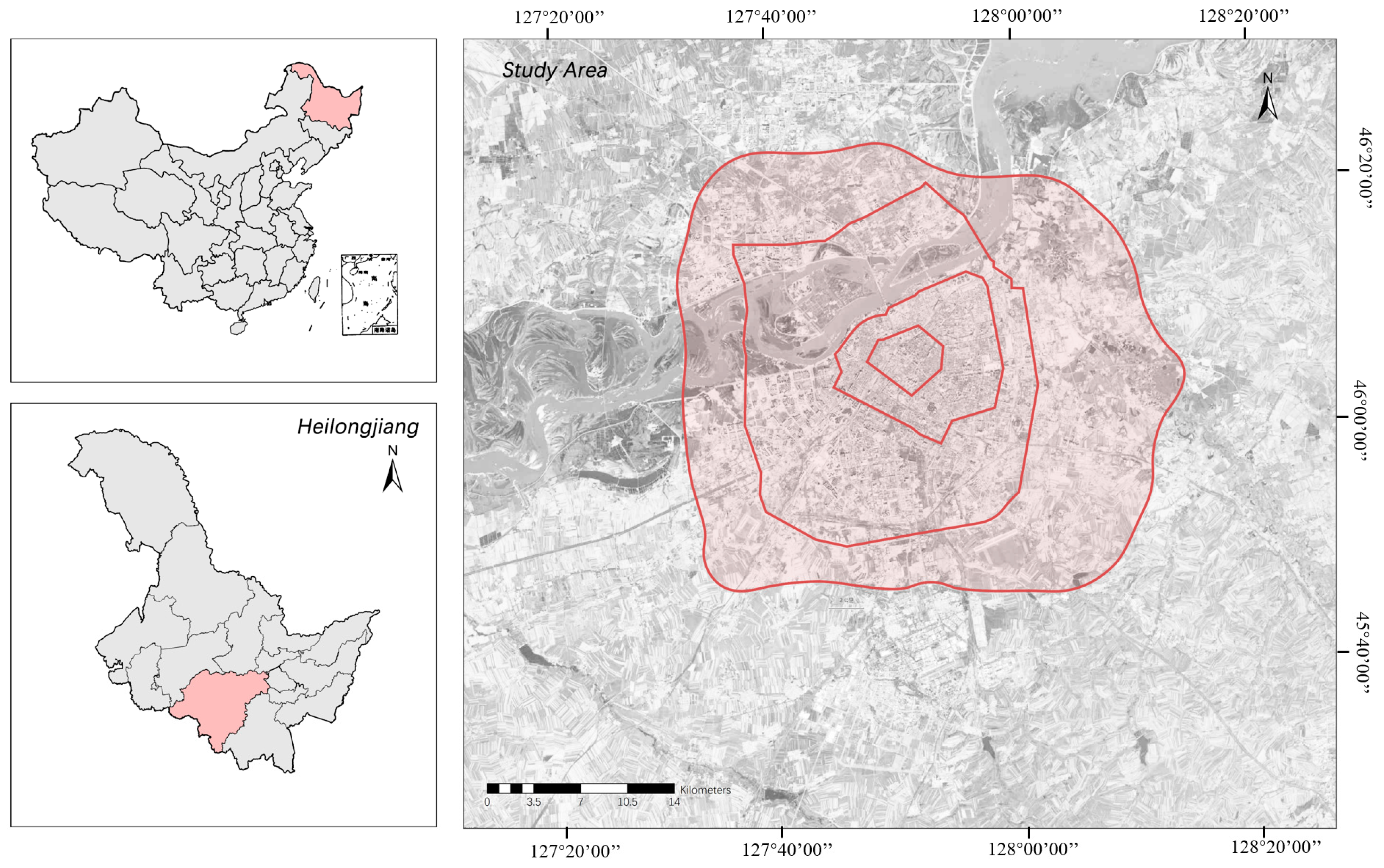
Harbin is located between 125°41′–130°13′ east longitude and 44°03′–46°40′ north latitude and is the capital of Heilongjiang Province. It is located in a midtemperate continental monsoon climate and severe cold region. Summer has average daily high temperatures of more than 19 °C. July has the highest temperatures, with an average high temperature of 27 °C and an average low temperature of 19 °C. The winter heating period lasts up to 180 days, with average daily high temperatures below −5 °C. January has the lowest temperatures, with an average low temperature of −23 °C and an average high temperature of −13 °C (https://weatherspark.com/y/142116/Average-Weather-in-Harbin-China-Year-Round accessed on 29 April 2024). Harbin is an important political, economic, and cultural center in Northeast China. As an old industrial base in northeastern China, it has experienced rapid development of heavy industry since the 1850s, with a large amount of land development. However, societal evolution and the reform of national policies have resulted in the phasing out of heavy industry. Government policies have shifted to a more diversified economic structure, leading to an economic decrease in Harbin and a decrease in the population in the administrative jurisdiction of Harbin City.
Harbin City has 9 districts and 9 counties. The road layout is characterized by the first, second, third, and fourth ring roads. The primary built-up area of Harbin is located within the Fourth Ring Road, with a marked decrease in building density beyond this boundary. As most social activities occur within this ring, studying this region is essential to understanding the environmental impacts of recent urban development. This analysis will facilitate predicting future urban trends and provide detailed guidance for city planning. The study area is situated around 45°44′29” N latitude and 126°38′09” E longitudes and has a total area of approximately 592.3 sq. Km. The study area is shown in Figure 1.
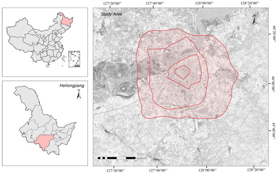
Figure 1.
Location of the research area.
2.2. Data Sources
Landsat multispectral images were obtained from the official website of the U.S. Geological Survey (http://earthexplorer.usgs.gov/ accessed on 15 December 2023). Multitemporal Landsat image series over Harbin City in 2005, 2010, 2015, and 2020 were downloaded. This study chose cloud-free images in summer (April, May, and June) and winter (December, January, and February). Table 1 lists the eight Landsat scenes (2 per year and 1 for each season). Since the image data of the study area were incomplete in some years, we used data from adjacent years as a substitute.

Table 1.
Landsat scenes used in this study.
2.3. LULC Classification
The Landsat images were classified into five LULC categories: (1) woodland and grassland (trees, parks, meadows, playgrounds, and other green vegetation), (2) cultivated land, (3) water land (rivers, lakes, and other small reservoirs), (4) urban land (residential, commercial, industrial, and transportation network areas), and (5) unused land.
The widely validated supervised classification method was used. Image analysts select pixels with known LULC labels to train a classification algorithm [23], which is used to classify the image pixels based on the predictor variable characteristics, and to construct parsimonious models of class label distributions [24].
The maximum likelihood (ML) method was used. It estimates the parameters of a probability function and assumes that the class training data in each band are normally distributed [25]. It is a widely used supervised classification method [26]. LULC identification is essential for assessing global, regional, and local environmental changes.
The classification process consisted of three steps: training sample selection, classification, and accuracy assessment [21]. This study collected more than 50 training samples for each LULC type. A pixel-based classifier was utilized to classify the images based on similar or identical spectral reflectance characteristics [27]. The region of interest (ROI) separability tool was used to calculate the statistical distance between the categories to determine the degree of dissimilarity. A separability value of >1.9 indicated a valid sample and a separability value of <1.8 indicated an invalid one. A separability value of < 1.0 meant that the samples were merged.
2.4. LST Inversion
Many methods have been used to compute LST, including the atmospheric correction method, Qin Zhihao single window algorithm, Offer Rosenstein split window algorithm, and Juan C. Jiménez-Muñoz split window algorithm among others [28]. This study chose two algorithms: the statistical mono-window (SMW) algorithm based on Landsat 5 satellite data and implemented in Google Earth Engine (GEE) [29] and the single-window surface temperature inversion algorithm based on Landsat 8 satellite data [30].
The SMW algorithm [27] is based on an empirical relationship between the top of the atmosphere (TOA) brightness temperature and the surface temperature obtained from the thermal infrared band. This study obtained the LST from Landsat 5 satellite data for Harbin City, in 2005 and 2010. The calculation formula of LST using Landsat5 images is shown in 1, 2, and 3:
where denotes the TOA brightness temperature in the Landsat thermal infrared channel and represents the surface emissivity obtained from the same channel. Parameters , , and are derived from linear regressions based on radiative transfer simulations. These simulations were conducted for 10 categories of the total column water vapor (TCWV), ranging from 0 to 6 cm in increments of 0.6 cm. The TCWV values exceeding 6 cm were classified as the category with the highest values.
where and are the NDVI values for fully bare and fully vegetated pixels, respectively; the emissivity values for vegetated areas at any given time can be derived using the vegetation cover method with the following formula:
where and are the emissivity of vegetation and bare ground for a given spectral band b.
This study used the single-window surface temperature inversion algorithm [28] to calculate the LST from Landsat 8 satellite data in 2015 and 2020. The calculation formula of LST using Landsat8 images is shown in 4 to 10:
where is the true surface temperature;
a, b are constants: a = −67.355351 and b = 0.458606; and
C and D are intermediate variables. is the mean atmospheric action temperature (in K), and is obtained by the inverse function of Planck’s formula.
where denotes the surface-specific emissivity and t is the transmittance of the atmosphere on that day.
The mean atmospheric action temperature has the following linear relationship with the near-surface air temperature (typically 2 m) (units of and are in degrees K Fahrenheit)
where denotes the local air temperature at the time of remote sensing image acquisition.
where and are preset constants before the satellite launch.
2.5. Estimation of UTFVI
The UTFVI was used to evaluate temperature differences between cities. Since the UTFVI is correlated with LST, it has been widely used to assess thermal conditions in urban areas. The calculation formula is shown in 11:
where is the LST (degrees Celsius) of the pixel, and is the average LST of the target region.
The UTFVI was categorized into six classes, none (UTFVI < 0), low (0–0.005), medium (0.005–0.010), high (0.010–0.015), very high (0.015–0.020), and extremely high (UTFVI > 0.020) [31], representing six UHI conditions: excellent, good, normal, bad, worse, and worst. The values ranged from no UHI at < to the worst UHI conditions at > [32].
2.6. PLUS Model
The PLUS model is a meta-CA model based on raster data that has been used to simulate LULC changes at the patch scale. The PLUS model consists of a rule-based mining approach based on a Land Expansion Analysis Strategy (LEAS) and a CA model based on multiple Random Seeds (CARS). The LEAS module utilizes the Random Forest algorithm to determine the degree of contribution of the factors affecting the expansion of LULC types between two periods and the probability of LULC types. The CA model predicts the evolution of LULC types at the patch level with high accuracy [16].
This study used the land use data of the built-up areas in Harbin City from 2005 to 2020 as the base layer. Since natural and socioeconomic factors affect LULC changes, this study selected six indicators to calculate the probability of LULC change using the LEAS module: digital elevation model (DEM), slope, and aspect for natural factors and distance from national and provincial highways and population density for social factors.
The weights indicated the expansion capacity of the land use type. They ranged from 0 to 1, with a larger value indicating a higher expansion capacity [16]. They were assigned based on the proportion of land use expansion area. The weights of woodland and grassland, cultivated land, urban land, water land, and unused land were 0.41, 0.45, 1, 0.1, and 0.15.
The transformation cost matrix was used to assess the conversion of land use types. The values were 0 or 1, with 0 indicating no conversion and 1 indicating conversion. The matrix was based on the conversion of LULC types in the study area in the Harbin City Roundabout Expressway from 2005 to 2020. Expert opinion, policies of returning farmland to forests and grassland, land reclamation in recent years, and urbanization were considered. The transformation cost matrix is presented in Table 2.
Table 2.
Transformation Cost Matrix.
The land use data in 2010 and 2015 were used as the base data, and those in 2015 and 2020 were simulated using the CARS module. The Kappa coefficient, overall accuracy, and the figure of merit (FOM) coefficient were used to evaluate the simulation accuracy and assess model performance for predicting land use in the study area. Using the Markov model integrated within the PLUS model, this study predicts the LULC types in the study area in 2025 and 2030, based on the 2020 land use data, and ensures the model’s accuracy meets the requirements.
2.7. Bi-LSTM Model
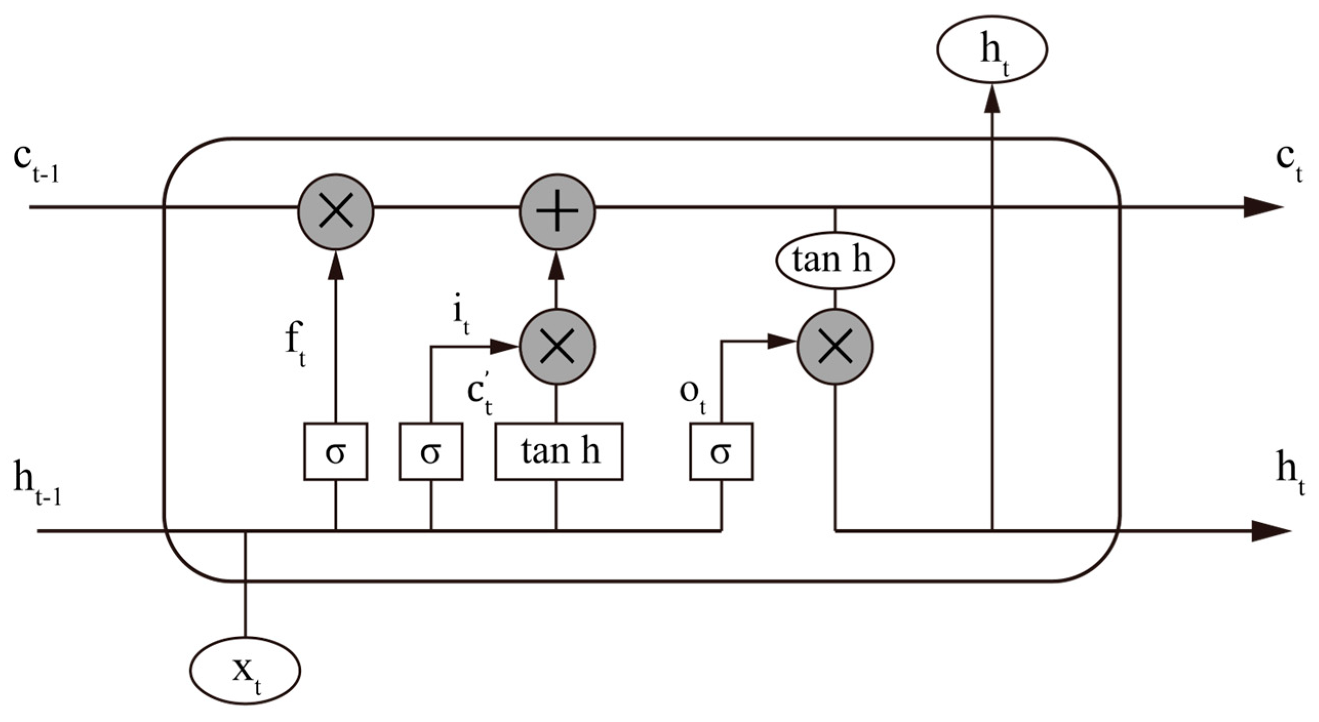
RNNs are used to extract information from time series data using historical and feature information to predict future conditions. However, they suffer from gradient explosion and vanishing. LSTM is a variant of an RNN that contains a memory module to prevent the loss of historical information [33]. Therefore, LSTM is more suitable for predictions using time series data, such as LST.
LSTM has three gate structures: a forget gate, an input gate, and an output gate. Its structure is shown in Figure 2, where f, i, c, and o represent the forget gate, input gate, cell state, and output gate, respectively; ct denotes the cell state at moment t, xt denotes the input at moment t, and ht denotes the output at the current moment, representing the input of the next cell state. σ is the Sigmoid activation function, providing an output ranging from 0 to 1, and tanh is a hyperbolic function, resulting in an output ranging from −1 to 1. ft, it, and ot denote the output states of the forget, input, and output gates, respectively. Its equation is (12) to (17), as follows:
where are the weight parameter, and are the bias parameter.
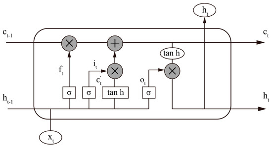
Figure 2.
LSTM unit internal structure.
Bi-LSTM is an optimized version of LSTM. It contains a hidden layer that transfers information in the reverse direction [34]. The forward layer calculates and records the output of each moment in positive order from the beginning to the end, whereas the reverse layer does the opposite. An activation function combines the results of the two layers into an output. Bi-LSTM has lower errors than LSTM because the output of the current moment is related to the historical and future time series data [35].
This study used the Bi-LSTM to predict the seasonal LST of Harbin in 2025 and 2030 using images from 2000, 2005, 2010, 2015, and 2020. To reduce the influence of daily temperature variations on our data, we standardized the Land Surface Temperature (LST) values when forecasting future LST using data from 2005 to 2020. We normalized the LST by using the average daily temperatures of the imagery dates: 20.44 °C in summer and −14.21 °C in winter. This approach minimizes the effect of day-specific temperatures, enhancing the accuracy of our predictive model. To reduce the data volume, this study resampled the images to 210 m resolution. Each image had 13,428 temperature data points. This study utilized 29,856 × 5 data points for 5 years as the training set and 1000 data points for 2020 as the test set. The number of iterations per round after 10 rounds of training was 3232, and the learning rate was 0.08. The and root mean square error (RMSE) were used to assess the prediction accuracy. The EXCEL data were imported into the GIS, and the resolution of the predicted and learning images was adjusted using radial basis functions (RBFs). This method considers the spatial correlation of the variables to ensure high-accuracy interpolation results. The final resolution was 30 m, which is consistent with the accuracy of the previous remote sensing image and is convenient for subsequent analysis and research.
3. Results
3.1. LULC Prediction and Trend Analysis
This study used the maximum likelihood method in ENVI 5.3 to classify the LULC types in the Harbin study area from 2005 to 2020. The overall accuracy rates were 91.19%, 94.40%, 90.72%, and 94.05%, and the Kappa coefficients were 0.8468, 0.8208, 0.8168, and 0.8626, indicating high classification accuracy.
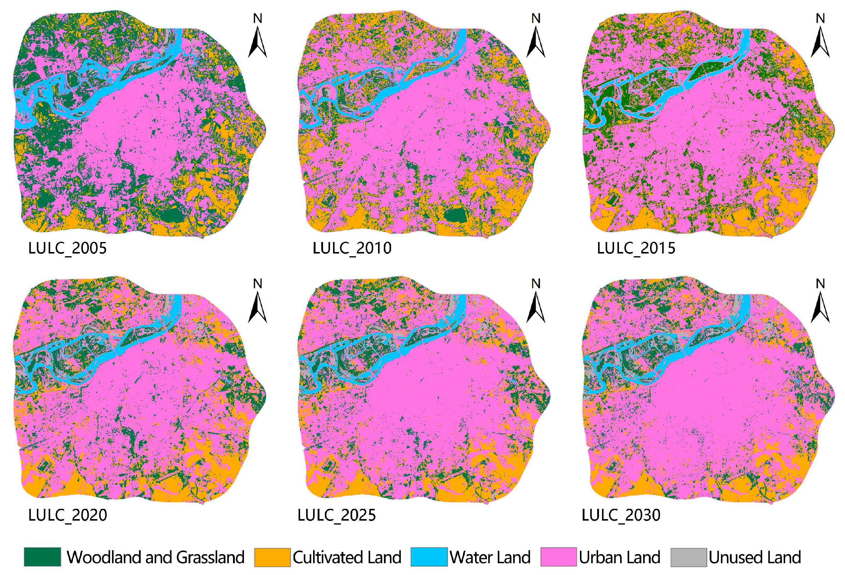
Figure 3 shows the classification and prediction of LULC from 2005 to 2030. The central area of Harbin expanded outward each year from 2005 to 2020, but the expansion rate decreased over time. This study used the PLUS model to predict the LULC of the Harbin built-up area in 2025 and 2030. This study utilized the LULC data of 2010 and 2015 to predict LULC changes in 2020 and compared the 2020 LULC predicted by the PLUS model with the actual 2020 LULC to verify the classification accuracy. Since the Kappa coefficient relies on LULC data and interval metrics, the FoM coefficient provides a more effective measure of the goodness of fit for simulating changes in landscape composition [36]. Thus, the FoM coefficient is chosen to validate the model’s accuracy. The FoM coefficient was 0.15, indicating high prediction accuracy. Therefore, this study could use the PLUS model to predict LULC changes in 2025 and 2030.
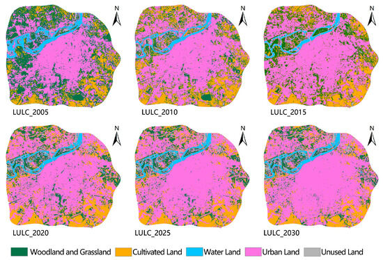
Figure 3.
Classification and prediction of LULC.
Due to extensive development and construction, the woodland and grassland on the north bank of the Songhua River was transformed into cultivated land and urban land from 2005 to 2030. Figure 4 shows the changes in the LULC types in Harbin City from 2005 to 2030. The area of urban and unused land increased, the area of cultivated land remained the same, and the area of water land, woodland, and grassland land decreased. The urban land area increased from 279.73 km2 to 387.50 km2, with a growth rate of 27.81%. Cultivated land increased from 80.57 km2 in 2005 to 140.58 km2 in 2015 and decreased to 90.27 km2 in 2030. Woodland and grassland exhibited the largest decreases from 2005 to 2030 (from 193.08 km2 to 75.16 km2, with a rate of 61.07%). Water land showed the smallest decrease, from 32.56 km2 to 21.70 km2, with a decrease rate of 33.34%.
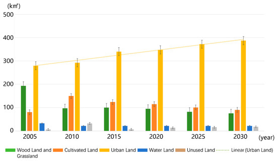
Figure 4.
Statistics of LULC changes.
3.2. LST Prediction and Trend Analysis
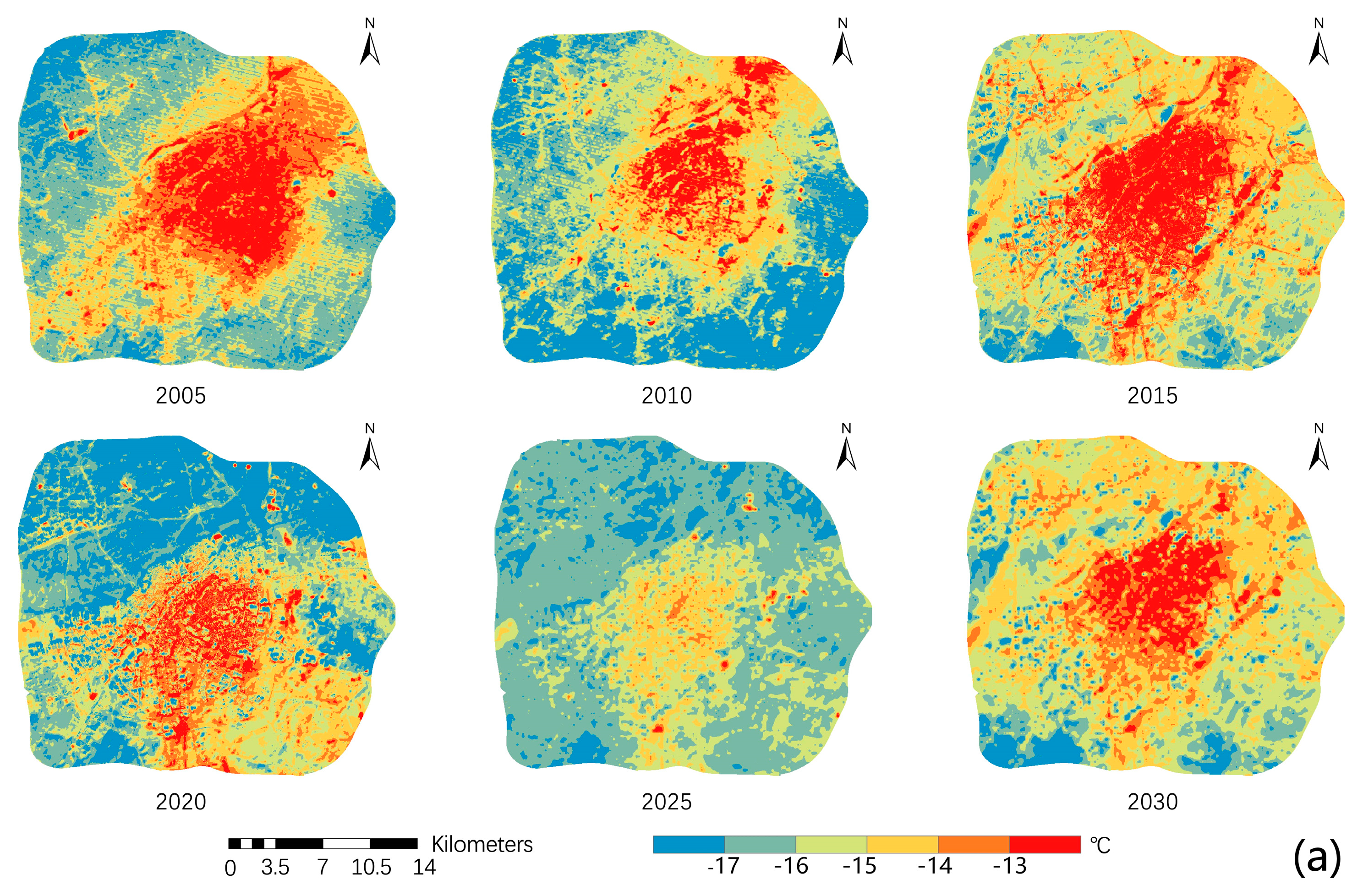
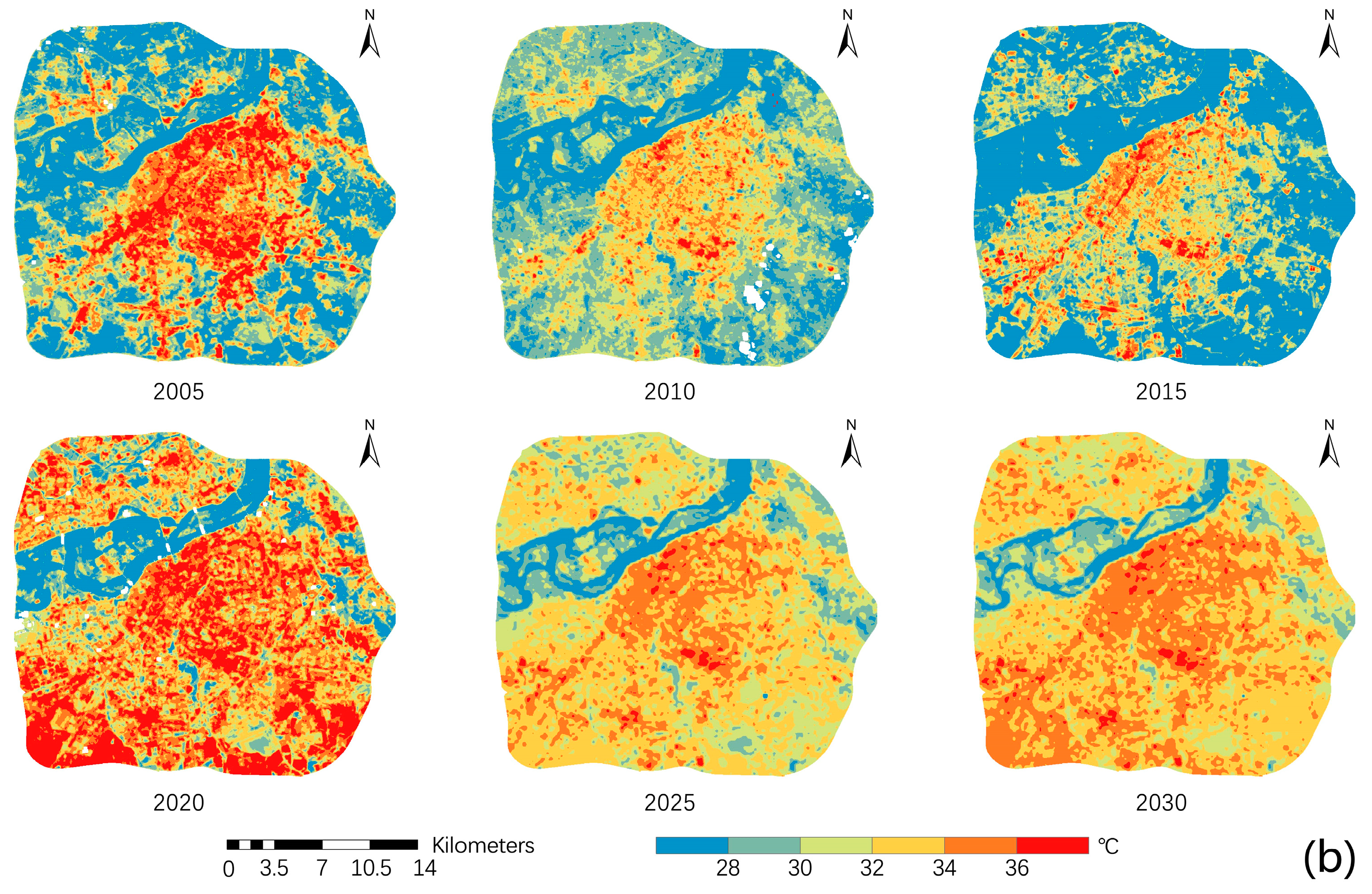
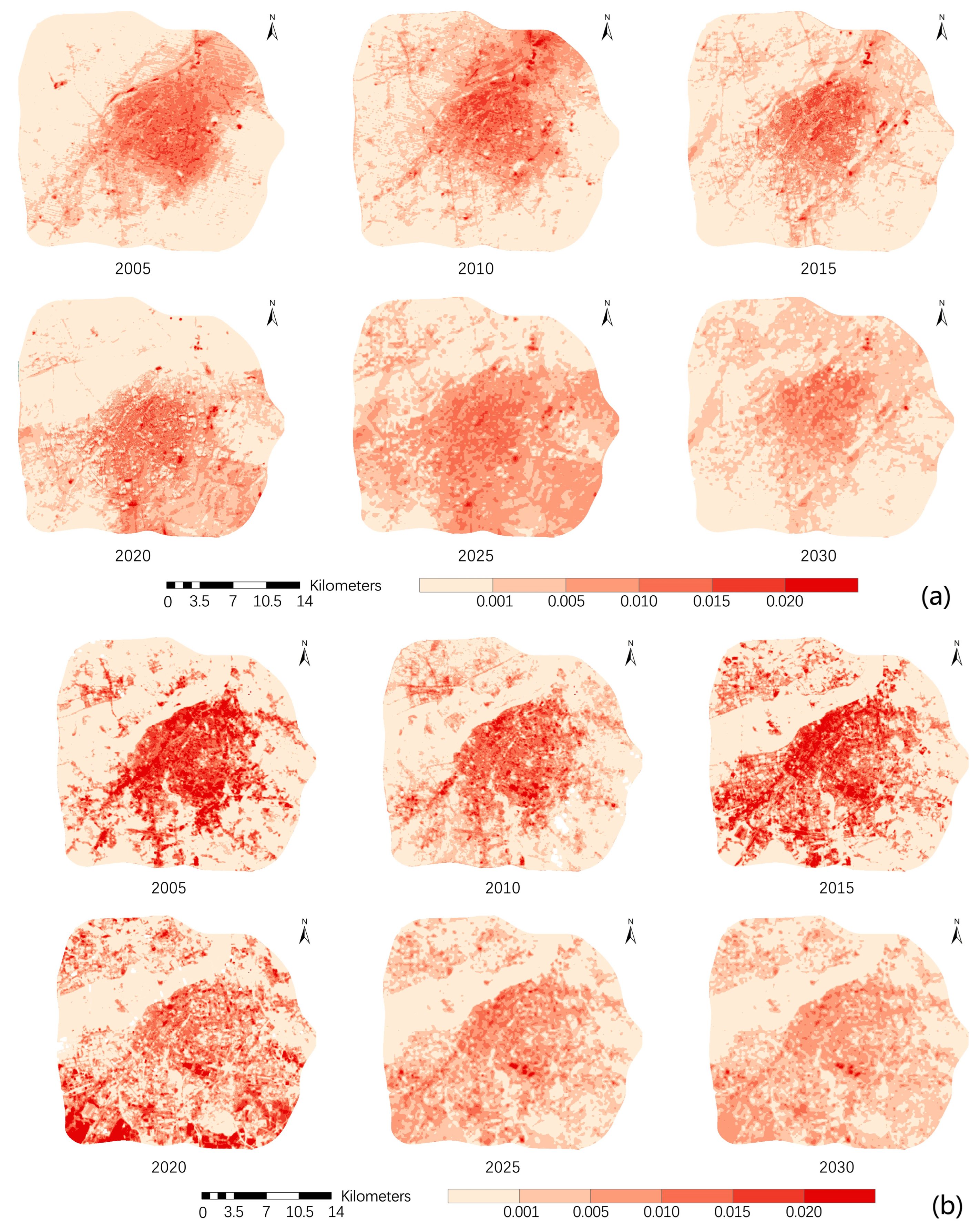
Figure 5 shows the distribution and prediction of LST in the study area from 2005 to 2030 in winter and summer. The winter and summer LSTs increased to different degrees from 2005 to 2020, and the high-temperature zone in summer expanded significantly. The for the winter predicted data for the Bi-LSTM model is 0.9953, and the RMSE is 0.1990. For the summer, the is 0.9498 and the RMSE is 0.3901, indicating accurate predicted results.


Figure 5.
Distribution and prediction of LST: (a) winter; (b) summer.
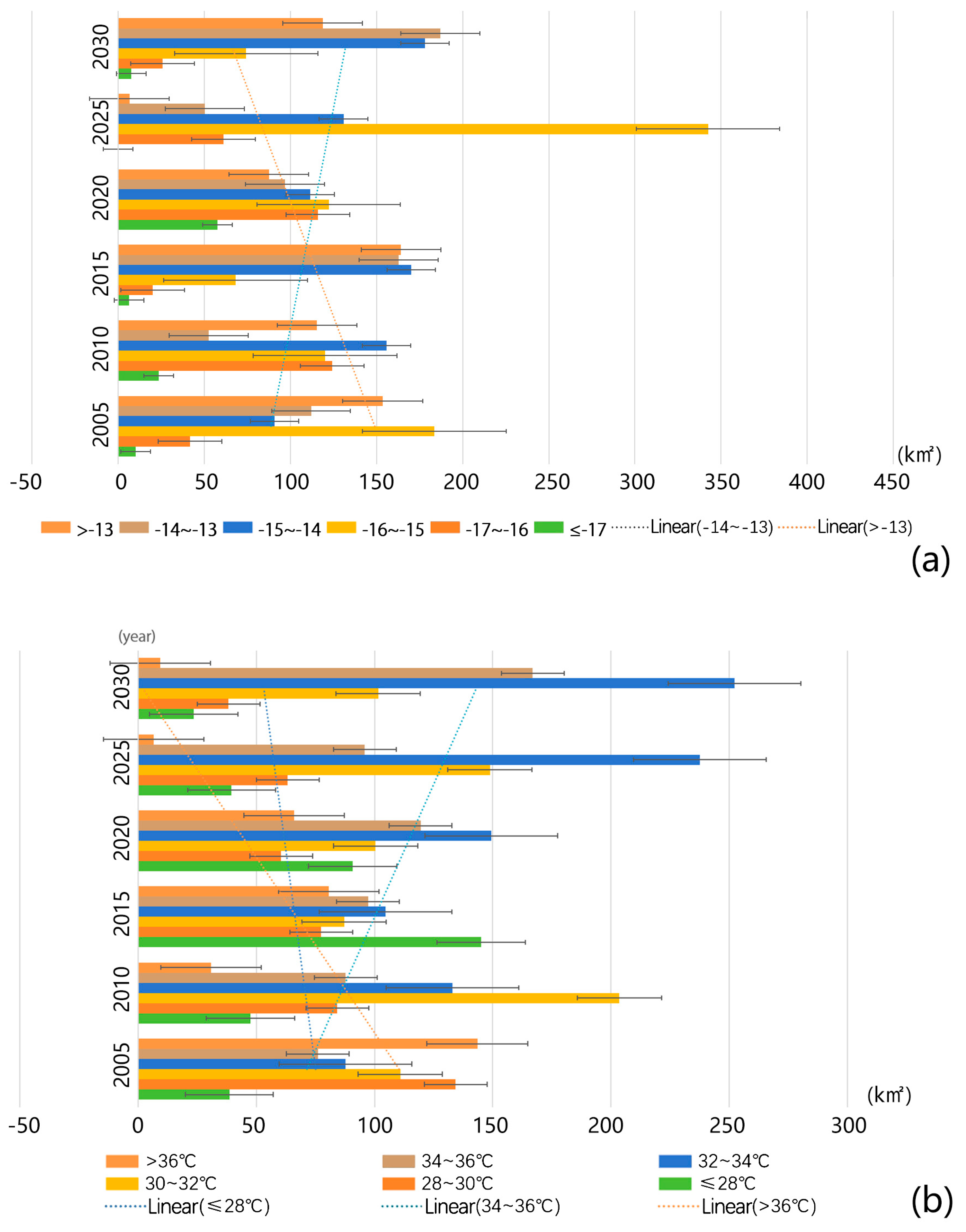
The change trends of LST in winter and summer from 2005 to 2030 are shown in Figure 6. During 2005–2030, the area decrease in the winter maximum temperature zone (LST > −13 °C) was the most significant, decreasing from 110.30 km2 to 43.03 km2, with a decreasing rate of 156.30%. The area of the low-temperature zone (LST ≤ −16 °C) and the medium-temperature zone (−14.9 °C–−14 °C) showed fluctuations. The area of the low-temperature zone (LST ≤ −16 °C) decreased from 235.66 km2 to 107.81 km2, with a decrease rate of 54.25%. The area occupied by the medium-temperature zone (−15.9 °C to −15 °C) and the high-temperature zone (−13.9 °C to −13 °C) increased steadily, with growth rates of 49.02% and 42.78%, respectively.
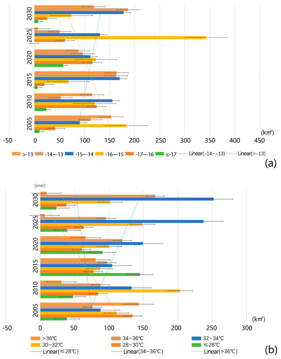
Figure 6.
Change trend of LST: (a) winter; (b) summer.
During 2005–2030, the area of the highest summer temperature zone (≥36.1 °C) decreased significantly from 143.49 km2 to 9.37 km2, with a decrease rate of 1430.99%. The area of the low-temperature zone (≤32 °C) decreased from 283.94 km2 to 163.359 km2 with a decrease rate of 42.27%. In addition, the area of the high-temperature zone (32.1 °C–36 °C) increased from 163.85 km2 to 419.17 km2 with a growth rate of 60.9%.
The area of the highest temperature zone in winter (LST > −13 °C) showed a decreasing trend from 2005 to 2030 with a decrease rate of 61.01%, whereas that of the high-temperature zone (−14.9 °C–−13 °C) rose significantly with a growth rate of 40.86%. A similar trend occurred in summer. The areas of the highest (LST > 36 °C) and lowest (LST ≤ 28 °C) temperature zones showed a decreasing trend with decrease rates of 93.7% and 39.06%, whereas the area of the high-temperature zone (34 °C–36 °C) showed an increasing trend with a growth rate of 60.9%. It can be concluded that the areas of high-temperature zones in winter and summer increased from 2005 to 2030, and those with extremely high temperatures showed a decreasing trend.
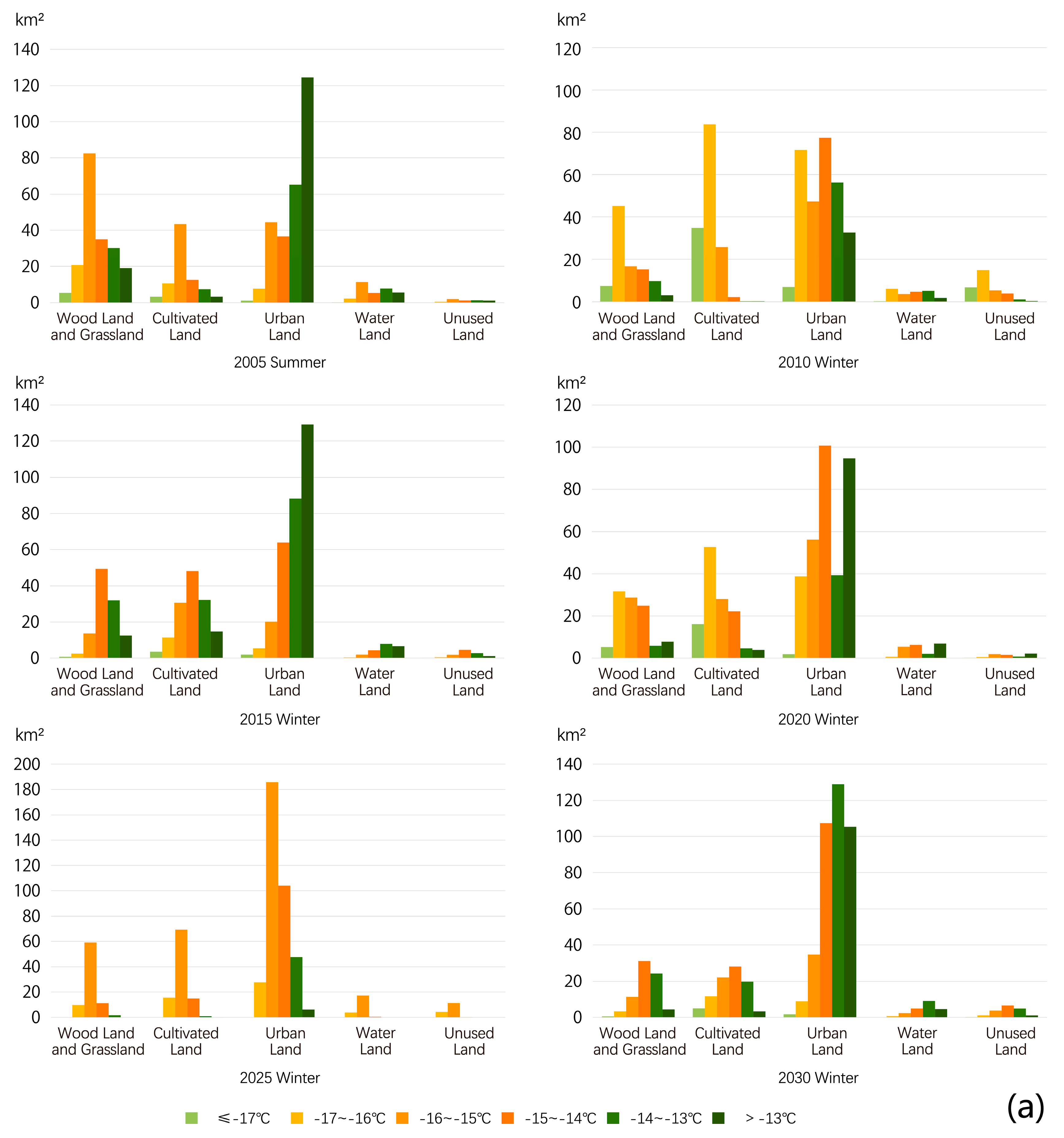
3.3. LST Distribution under Different LULC Classes
Figure 7 shows the seasonal LSTs for different LULC types during 2005–2030. As shown in Figure 7a, urban land had the highest temperatures in winter. The zones with temperatures in the range of −16 °C to −14 °C increased from 80.98 km2 to 142.06 km2, with a growth rate of 75.43%. The area of the highest temperature zone (LST > −13 °C) exhibited a fluctuating decreasing trend, with a decrease rate of 15.42%. The area of the lowest (LST ≤ −17 °C) and highest (LST > −13 °C) temperature zones for woodland and grassland showed a decreasing trend, with rates of 90% and 76.99%.


Figure 7.
LSTs for different LULC types: (a) winter; (b) summer.
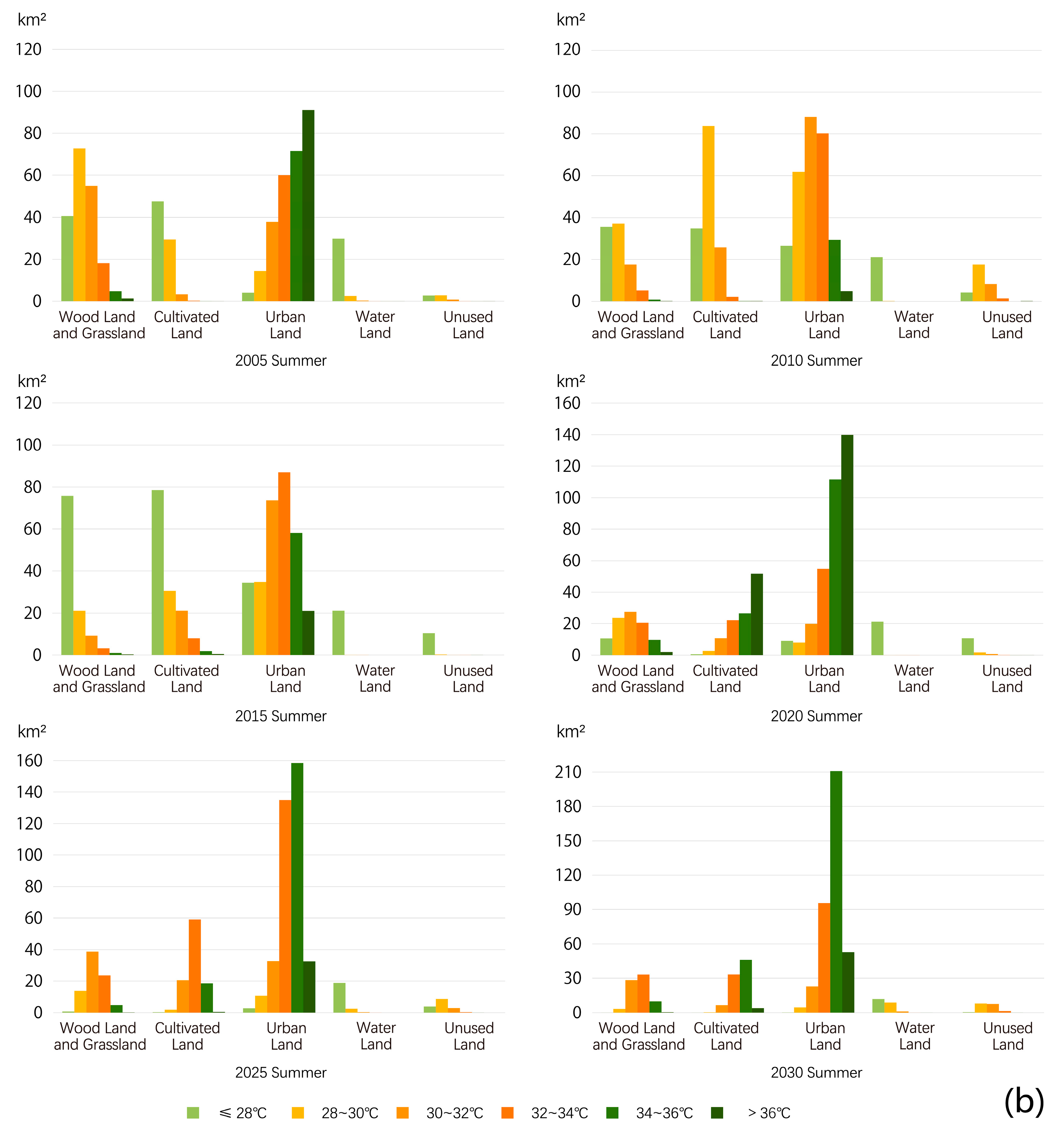
Figure 7b shows that the area of urban land in the high-temperature zone (LST > 34 °C) in summer increased from 162.74 km2 to 263.73 km2 with a growth rate of 62.06%. However, the area of urban land in the highest temperature zone decreased from 91.14 km2 to 52.84 km2 with a decrease rate of 42.02%. The area of water land in the lowest temperature zone (LST ≤ 28 °C) did not change significantly, but the one in the low-temperature zone (LST ≤ 28 °C) decreased from 32.56 km2 to 21.70 km2, with a decrease rate of 33.35%.
The change trend (increase and decrease) of the seasonal LST under different LULC types from 2005 to 2030 was similar for winter and summer, with the summer change extent being more significant. Urban land consistently exhibited significantly higher temperatures than other LULC types in winter and summer. The area of the high-temperature zone expands each year because nonevaporative surfaces, such as buildings and bare land, often exhibit higher surface temperatures than evaporative surfaces, such as water land and vegetation [37]. Woodland, grassland, and urban land showed similar trends in winter and summer, with a decrease in extremely high- and low-temperature zones, indicating a decrease in extreme temperatures.
3.4. Variation Analysis of Seasonal UTFVI
Figure 8 shows the seasonal UTFVI from 2005 to 2030, and Table 3 lists the area metrics. The highest UTFVI values in winter and summer were located in the central part of the city, and the no-UTFVI zone was located in the suburbs. The dividing line was clearer in summer than in winter. The no- (<0.000) and low- (0.000–0.005) UTFVI zones occurred in water land, woodland, grassland, and cultivated land. The area of the no-UTFVI zone (<0.000) in winter (summer) decreased from 326.64 km2 to 290.51 km2 (319.33 km2 to 230.25 km2), with a decrease rate of 11.06% (27.90%). UTFVI zones above high values (>0.010) decreased from 71.66 km2 to 1.28 km2 in winter with a decrease rate of 74.49% and from 151.72 km2 to 14.07 km2 in summer with a decrease rate of 90.73%. This phenomenon can be attributed to the gradual increase in average annual temperature, which reduces the temperature difference and consequently decreases the UTFVI value and weakens the UHI intensity. However, the urban thermal environment has not improved.
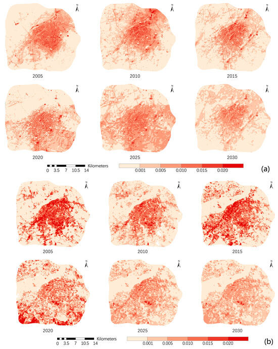
Figure 8.
Distribution of UTFVI zone: (a) winter; (b) summer.
Table 3.
Area (km2) distribution of seasonal UTFVI.
The seasonal distribution of the UTFVI shows that the area of the no-UTFVI zone (<0.000) decreased each year, and the effect was more pronounced in winter than in summer. In contrast, the area with the extremely high UTFVI values showed a decreasing trend, with slight fluctuations in summer. The area was very small by 2030 (0.02% in winter and 0.08% in summer). This result indicates a decrease in the range of extremely high temperatures in the study area due to urban construction and climate change.
3.5. UTFVI Variation over Different LULC Classes
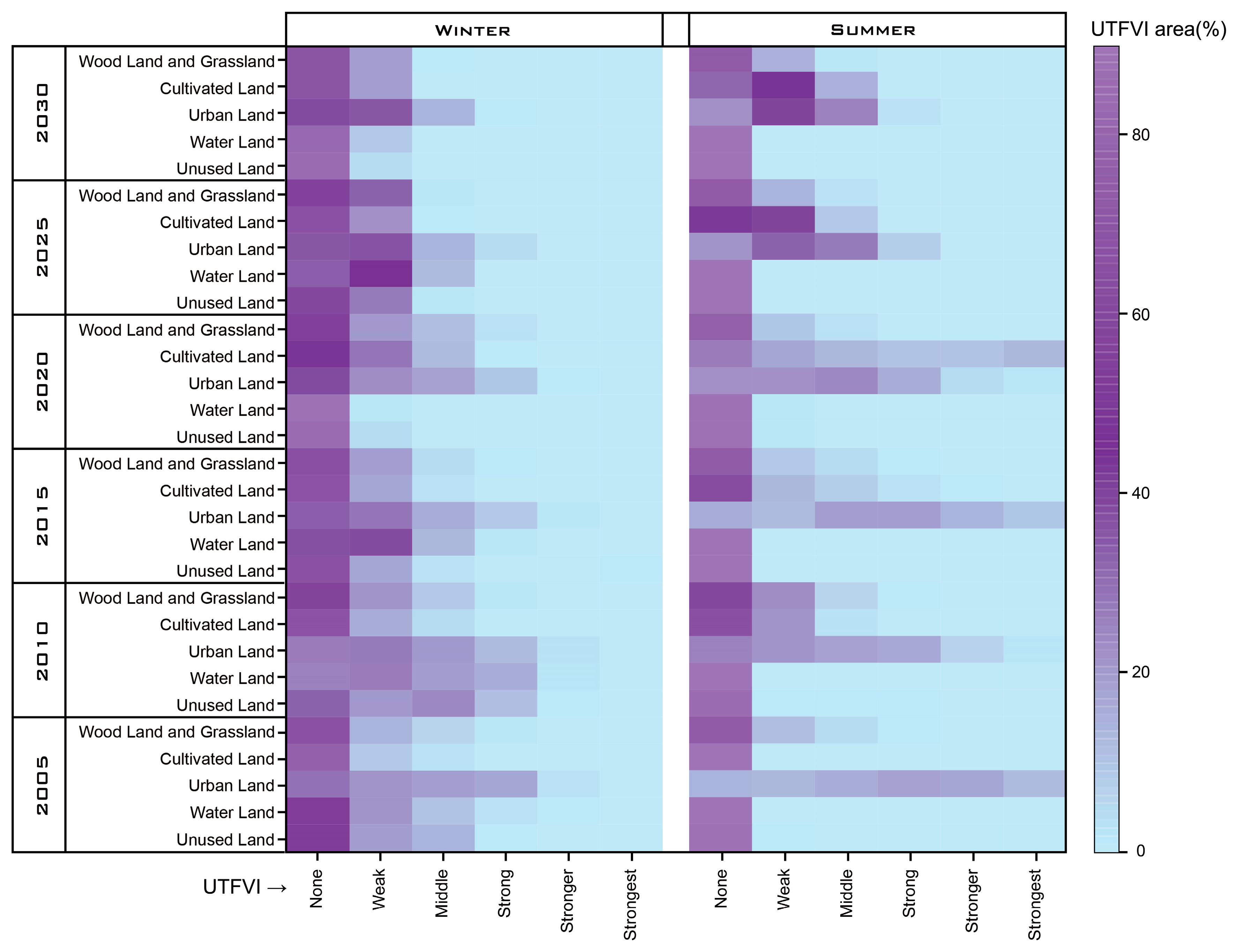
Figure 9 shows the distribution of UTFVI zones for different LULC types from 2005 to 2030. The UTFVI values are the highest for urban land in summer, and the no-UTFVI zone occurs in all LULC types.
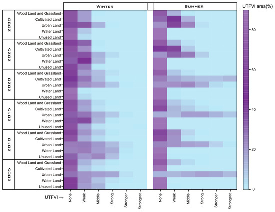
Figure 9.
Distribution of U’TFVI zones over different LULC classes during winter and summer seasons.
The no- (<0.000) and low- (0.000–0.005) UTFVI zones were dominant in woodland, grassland, cultivated land, water land, and unused land, and their proportions were 83.19–93.47%, 84.91–99.05%, 83.20–99.93%, and 81.58–98.76%, respectively. The proportion of UTFVI values in the medium and above (>0.005) zones in urban land decreased from 44.52% to 17.84%, with a decrease rate of 59.93%.
The no- (<0.000) UTFVI zone of woodland and grassland in summer was dominant, with a proportion of about 80% in all years except for 2010. The annual trend of cultivated land was not significant. The proportion of the area in the medium UTFVI zone and above (>0.010) in urban land decreased from 70.39% to 32.23%, with a decrease rate of 54.21%. The proportion of the area in the medium UTFVI zone (0.005–0.010) increased from 17.87% to 28.72%, with a growth rate of 50.71%. The proportion of the high UTFVI zone (0.010–0.015) decreased from 20.14% to 3.08%, with a decrease rate of 84.70%. The UTFVI values of water land and unused land changed steadily. The UTFVI (<0.000) zone was dominant, and the proportions were 97.76–99.99% and 95.03–99.29% for water land and unused land, respectively.
The results indicate that the UTFVI values of woodland, grassland, cultivated land, water land, and unused land did not change significantly over time. The UTFVI values of urban land exhibited larger changes in summer. The proportion of the medium-UTFVI zone (0.005–0.010) rose, whereas that of zones higher than the medium value (>0.005) decreased, indicating that the area affected by the UHI decreased, while the UHI intensity in some regions increased, and the quality of the urban thermal environment worsened.
4. Discussion
4.1. Validation of the Accuracy of the Bi-LSTM Model
Recently, machine learning algorithms have been widely used in remote sensing prediction. To predict future LSTs, this study compared different algorithms to predict future LSTs (Table 4): linear regression, support vector machine, Decision Tree, Random Forest, and Bi-LSTM. These algorithms have been used in recent remote sensing prediction studies. This study chose the validation mean absolute error (MAE), , and RMSE to evaluate model accuracy. This study selected 2000, 2005, 2010, and 2015 as input data to predict the 2020 LSTs and compared different models. The results show that Bi-LSTM outperformed the other algorithms, with a higher and lower validation MAE and RMSE values. Therefore, this study used Bi-LSTM for the prediction.
Table 4.
Accuracy evaluation of each model.
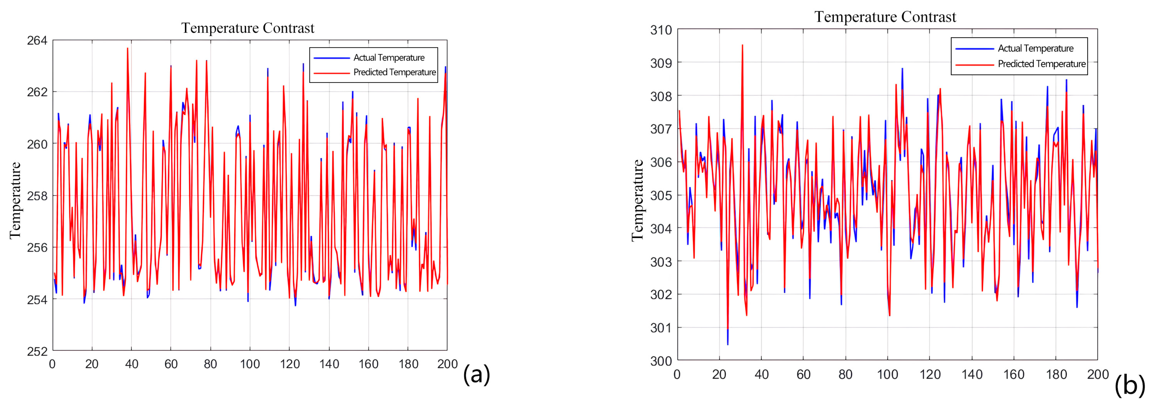
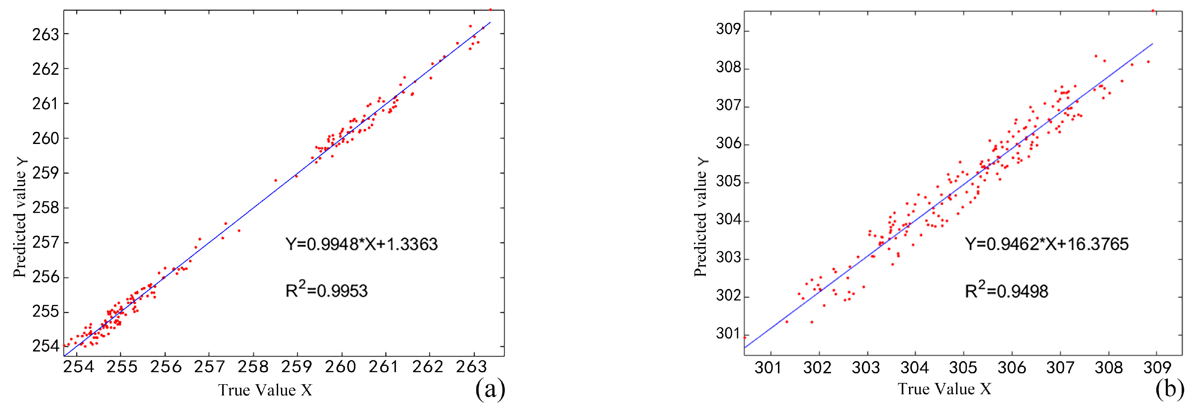
Figure 10 illustrates the comparison between predicted and actual values on the validation set of the Bi-LSTM model, indicating minimal discrepancies. Figure 11 shows the fitted regression line. The is 0.9953 and 9498, and the RMSE is 0.1990 and 0.3901 for winter and summer, respectively, indicating accurate prediction results.
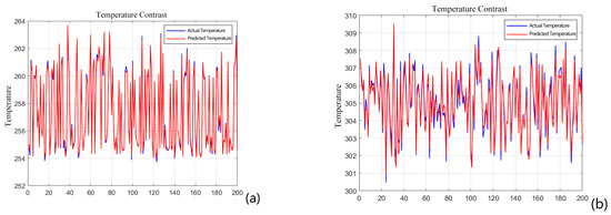
Figure 10.
Comparison of actual and predicted temperatures: (a) winter; (b) summer.
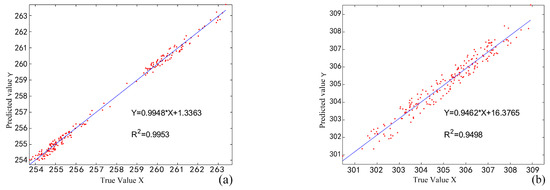
Figure 11.
Fitted regression line of LST: (a) winter; (b) summer.
From Figure 5, it is evident that the distribution of Land Surface Temperature (LST) during the winter of 2025 differs in the high-temperature areas compared with other years. The Bi-LSTM model was trained using data from 2000 to 2020, with the LST image from winter 2000 shown in Figure 12. Temperature variations exhibit periodicity, with the LST image of 2025 resembling that of 2000. Training large models is significantly influenced by the training dataset, especially for complex deep learning models, which exhibit inherent unpredictability. The distribution of high- and low-temperature areas in the LST image of winter 2025 aligns with expected patterns, indicating a high predictive accuracy of the model. The graphical representation, with temperature intervals divided into 1 °C increments, shows minimal differences between the LST image of winter 2025 and previous years, affirming these results as normal and accurate. In addition, this study does not fully consider climate change or multiscenario simulations when predicting LULC and LST, which presents certain limitations. These aspects will be addressed in future research.
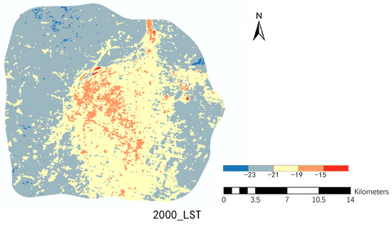
Figure 12.
Winter 2000 LST Image.
4.2. Strategies to Mitigate UHI in the Central City Area
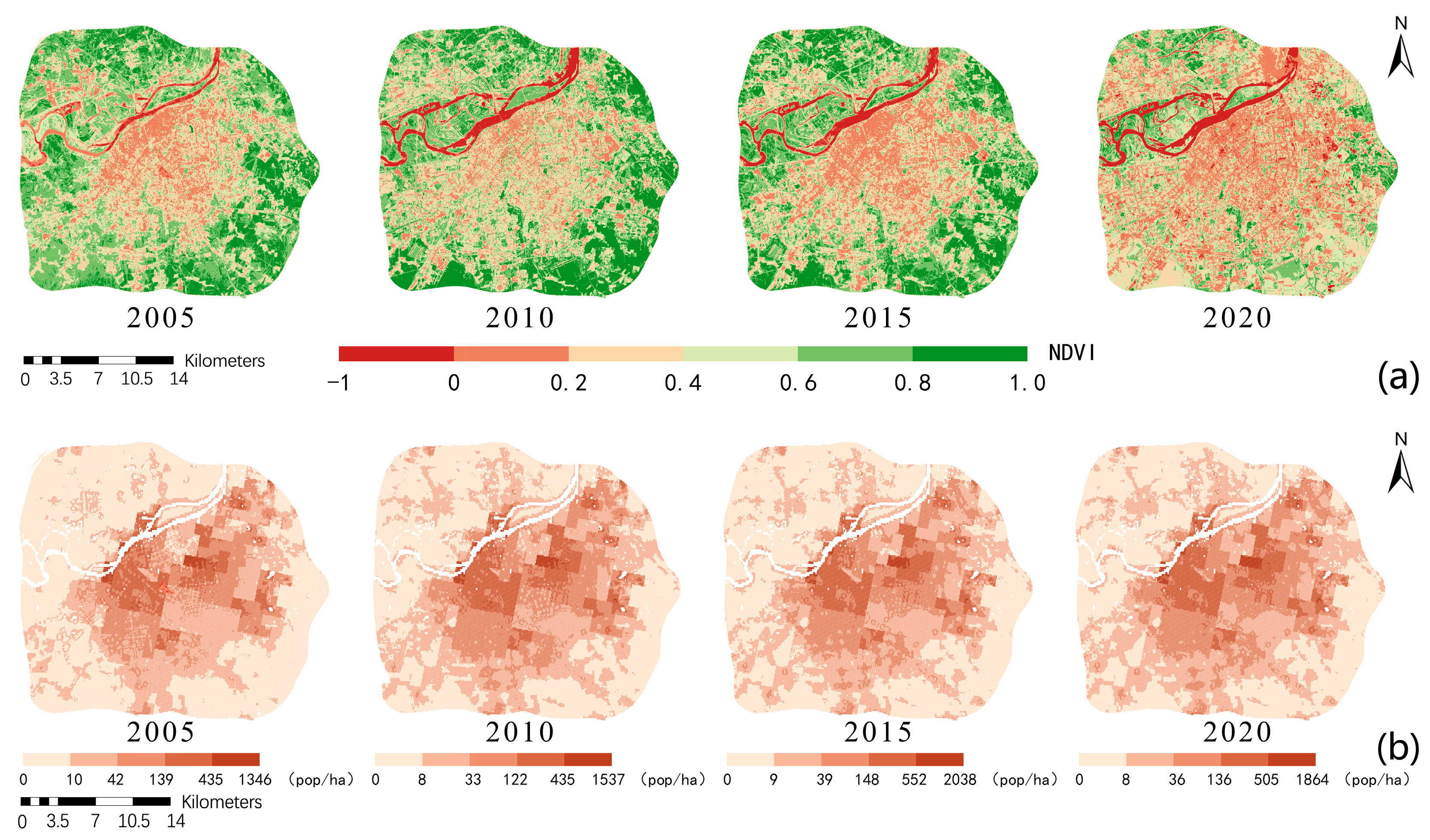
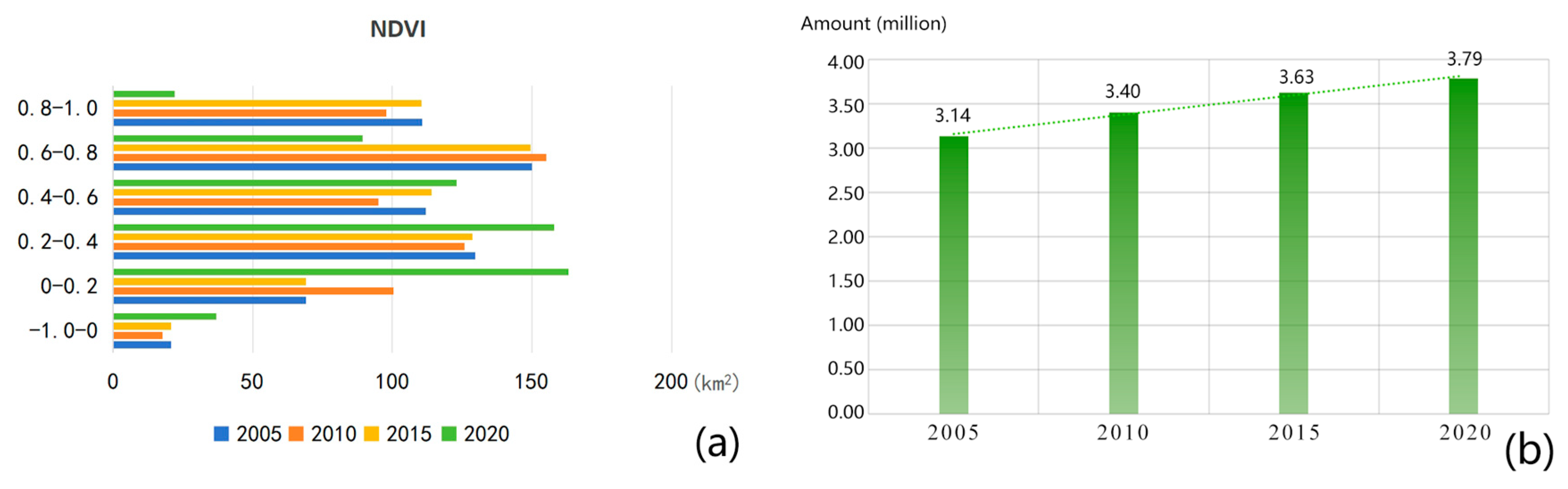
This study conducted spatial and temporal monitoring of LULC types, LST, and UTFVI in the built-up area of Harbin City using Landsat images from 2005 to 2020 and predicted conditions in 2025 and 2030. This study analyzed the relationship between LULC change and LST, UTFVI, and UHI from 2005 to 2030. The results showed that urban land expanded from 2005 to 2030. Areas with higher LSTs increased, and those with extremely high LSTs decreased. An increase in the high-temperature zones increased the average temperature, resulting in a decrease in the temperature difference and anomalous changes in the UTFVI. Areas with high UTFVI values were located in urban areas, and the proportion of zones with medium UTFVI values and above (>0.010) in urban areas decreased each year. The proportion of zones with medium UTFVI values (0.005–0.010) increased, and the proportion of areas with medium UTFVI values and above (>0.005) decreased, indicating that the area affected by the UHI has decreased, the UHI intensity in some regions has increased, and the quality of the urban thermal environment has worsened. A decrease in vegetation cover and an increase in population size affect the UHI. Li [38] found that rapid urban expansion resulted in decreases in the NDVI, increasing the UHI index. Priyadarsini [39] observed that an increase in human activities increased the UHI effect. Figure 13a and Figure 14a show that the area of high NDVI values zones (>0.2) decreased from 2005 to 2030, with a decrease rate of 21.93%, indicating a decrease in vegetation cover. Figure 13b and Figure 14b show that the population increased with a growth rate of 20.86%. This result confirms that the quality of the urban thermal environment has worsened. These findings indicate that the expansion of urban land and the reduction in woodland and grassland have exacerbated the UHI and the unsustainability of urban development. Therefore, it is necessary to reduce the expansion of urban land and increase the area of woodland and grassland or improve the vegetation cover to mitigate the UHI effect.
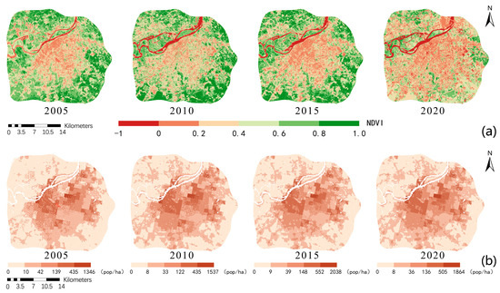
Figure 13.
(a) Distribution of NDVI. (b) Distribution of population.
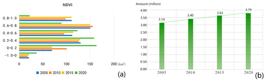
Figure 14.
(a) Change trend of NDVI. (b) Change trend of population.
The changes in LULC and LST observed in our study from 2005 to 2030 differ from those observed in other studies. For example, Zhang [40] conducted a study in Wuhan (which is located in the central part of China in a subtropical monsoon climate zone; it is the capital of Hubei Province and is a megacity). They found that the high-temperature zone (LST > 27 °C) in Wuhan’s urban area expanded, whereas the areas of woodland, grassland, and water land in the low-temperature area decreased [41]. These changes exacerbated the rise in LSTs in central urban areas and reduced thermal comfort [42]. This study area, distinct from Wuhan City’s temperature zone, displays an expansion in high-temperature zones and a contraction in extreme-temperature areas. The differences observed between Harbin and Wuhan highlight variations in urban spatial scale, climatic characteristics, spatial layout, LULC, and urban morphology. For instance, Harbin’s urban form, influenced by sunlight exposure and energy-saving requirements, exhibits significant differences in building spacing, volume, and layout compared with Wuhan. These factors contribute to distinct trends and intensities in UHI effects, which also display seasonal and regional variations. This regional study underscores the importance of understanding such localized dynamics.
Most studies have focused on cities in tropical and subtropical climates in East Asia, Southeast Asia, and Africa, whereas studies of cities in temperate zones are relatively rare. This study fills this research gap by investigating a typical city, Harbin, in a cold region, providing crucial insights for similar research on LULC and UHI.
5. Conclusions
This study used Harbin, a city in the severe cold region, as a case study to predict LULC change using the PLUS and Bi-LSTM models to predict LSTs in 2025 and 2030. The trends of LULC change, seasonal LST, and seasonal UTFVI from 2005 to 2030 were analyzed. The effects of LULC change on LST and UTFVI were evaluated to assess the impact on the UHI effect. The following conclusions were drawn:
- This study established a Bi-LSTM model to predict seasonal LSTs. The and RMSE values were 0.9953 and 0.1990 in winter and 0.9498 and 0.3901 in summer, indicating high prediction accuracies and outperforming the other models.
- The area of urban land increased from 2005 to 2030, with a growth rate of 27.81%. The area of woodland and grassland decreased at a rate of 61.07%, and the area of water land and unused land remained stable, indicating that the urban land will continue to expand gradually in the future.
- The surface temperature inversion results and the Bi-LSTM model prediction results show a decrease in the area of the extreme temperature zone in winter and summer and an increase in the area of the highest temperature zone from 2005 to 2030. The area of the highest temperature zone (LST > −13 °C) in winter had a decrease rate of 61.01%, and the growth rate of the area of the high-temperature zone (−14.9 °C to −13 °C) was 40.86%. The rates of decrease in the areas of the highest (LST > 36 °C) and lowest (LST ≤ 28 °C) temperature zones in summer were 93.47% and 39.06%, and the growth rate of the area with the high-temperature zone (32 °C–36 °C) was 60.9%. The area with the lowest LST (≤−16 °C) was transformed into an area with high LSTs (−14.9 °C–−13 °C). Urban land with high temperatures (LST > 34 °C) expanded with a growth rate of 62.06%. LULC change due to urban development and expansion led to increases in LSTs.
- UTFVI zones above high values (>0.010) decreased from 2005 to 2030, with a reduction rate of 90.73%. Zones with high UTFVI values were located in urban land, and this effect was more pronounced in summer. The proportion of areas with medium UTFVI values zones (0.005–0.010) in urban land increased at a rate of 50.71%. In contrast, the proportion of areas with medium UTFVI values and above (>0.005) decreased at a rate of 84.70%. This result shows that the area affected by the UHI has decreased, the UHI intensity in some regions has increased, and the quality of the urban thermal environment has worsened.
This study demonstrates that Landsat 5 and 8 satellite data are suitable for assessing the relationship between LULC change, LST, and UTFVI in Harbin City. It is recommended to mitigate the UHI effect by increasing the area of woodland and grassland or vegetation cover. Suitable land use is required to ensure urban thermal comfort. Our results can be used to improve urban planning strategies in severe cold regions to manage urban thermal environments and enhance urban livability.
Author Contributions
Conceptualization, X.Y. and P.C.; methodology, S.L. and P.C.; software, S.L.; validation, S.L., Y.S. and B.S.; formal analysis, S.L.; investigation, S.L.; resources, S.L.; data curation, S.L. and Y.S.; writing—original draft preparation, Y.S. and B.S.; writing—review and editing, S.L.; visualization, Y.S., B.S. and S.L.; supervision, X.Y. and P.C.; project administration, X.Y.; funding acquisition, P.C. All authors have read and agreed to the published version of the manuscript.
Funding
This research was funded by the Fundamental Research Funds for the Central Universities (grant number 2572023CT18-06) and the Natural Science Foundation of Heilongjiang Province of China (YQ2023E003).
Data Availability Statement
The original contributions presented in the study are included in the article; further inquiries can be directed to the corresponding author.
Conflicts of Interest
The authors declare no conflicts of interest.
References
- Hassan, T.; Zhang, J.; Prodhan, F.A.; Sharma, T.P.P.; Bashir, B. Surface urban heat islands dynamics in response to LULC and vegetation across South Asia (2000–2019). Remote Sens. 2021, 13, 3177. [Google Scholar] [CrossRef]
- Al Kafy, A.; Rahman, S.; Faisal, A.-A.; Hasan, M.M.; Islam, M. Modelling future land use land cover changes and their impacts on land surface temperatures in Rajshahi, Bangladesh. Remote Sens. Appl. Soc. Environ. 2020, 18, 100314. [Google Scholar]
- Mohammad, P.; Goswami, A. Predicting the impacts of urban development on seasonal urban thermal environment in Guwahati city, northeast India. Build. Environ. 2022, 226, 109724. [Google Scholar] [CrossRef]
- Goldblatt, R.; Addas, A.; Crull, D.; Maghrabi, A.; Levin, G.G.; Rubinyi, S. Remotely sensed derived land surface temperature (LST) as a proxy for air temperature and thermal comfort at a small geographical scale. Land 2021, 10, 410. [Google Scholar] [CrossRef]
- Al Kafy, A.; Faisal, A.A.; Rahman, S.; Islam, M.; Al Rakib, A.; Islam, A.; Khan, H.H.; Sikdar, S.; Sarker, H.S.; Mawa, J.; et al. Prediction of seasonal urban thermal field variance index using machine learning algorithms in Cumilla, Bangladesh. Sustain. Cities Soc. 2021, 64, 102542. [Google Scholar] [CrossRef]
- Grigoraș, G.; Urițescu, B. Land use/land cover changes dynamics and their effects on surface urban heat island in Bucharest, Romania. Int. J. Appl. Earth Obs. Geoinf. 2019, 80, 115–126. [Google Scholar] [CrossRef]
- dos Santos, A.R.; de Oliveira, F.S.; da Silva, A.G.; Gleriani, J.M.; Gonçalves, W.; Moreira, G.L.; Silva, F.G.; Branco, E.R.F.; Moura, M.M.; da Silva, R.G.; et al. Spatial and temporal distribution of urban heat islands. Sci. Total Environ. 2017, 605, 946–956. [Google Scholar] [CrossRef]
- Zhang, M.; Zhang, C.; Kafy, A.-A.; Tan, S. Simulating the relationship between land use/cover change and urban thermal environment using machine learning algorithms in Wuhan City, China. Land 2021, 11, 14. [Google Scholar] [CrossRef]
- Gazi, Y.; Rahman, Z.; Uddin, M.; Rahman, F.M.A. Spatio-temporal dynamic land cover changes and their impacts on the urban thermal environment in the Chittagong metropolitan area, Bangladesh. GeoJournal 2021, 86, 2119–2134. [Google Scholar] [CrossRef]
- Hua, A.K.; Ping, O.W. The influence of land-use/land-cover changes on land surface temperature: A case study of Kuala Lumpur metropolitan city. Eur. J. Remote Sens. 2018, 51, 1049–1069. [Google Scholar] [CrossRef]
- Mumtaz, F.; Yu, T.; De Leeuw, G.; Zhao, L.; Fan, C.; Elnashar, A.; Bashir, B.; Wang, G.; Li, L.; Naeem, S.; et al. Modeling spatio-temporal land transformation and its associated impacts on land surface temperature (LST). Remote Sens. 2020, 12, 2987. [Google Scholar] [CrossRef]
- Wu, Z.; Zhang, Y. Spatial variation of urban thermal environment and its relation to green space patterns: Implication to sustainable landscape planning. Sustainability 2018, 10, 2249. [Google Scholar] [CrossRef]
- Wang, J.; Bretz, M.; Dewan, M.A.A.; Delavar, M.A. Machine learning in modelling land-use and land cover-change (LULCC): Current status, challenges and prospects. Sci. Total Environ. 2022, 822, 153559. [Google Scholar] [CrossRef] [PubMed]
- Cengiz, A.; Budak, M.; Yağmur, N.; Balçık, F. Comparison between random forest and support vector machine algorithms for LULC classification. Int. J. Eng. Geosci. 2023, 8, 1–10. [Google Scholar]
- de Souza, J.M.; Morgado, P.; da Costa, E.M.; de Novaes Vianna, L.F. Modeling of land use and land cover (LULC) change based on artificial neural networks for the Chapecó river ecological corridor, Santa Catarina/Brazil. Sustainability 2022, 14, 4038. [Google Scholar] [CrossRef]
- Liang, X.; Guan, Q.; Clarke, K.C.; Liu, S.; Wang, B.; Yao, Y. Understanding the drivers of sustainable land expansion using a patch-generating land use simulation (PLUS) model: A case study in Wuhan, China, Computers. Environ. Urban Syst. 2021, 85, 101569. [Google Scholar] [CrossRef]
- Mathew, A.; Sreekumar, S.; Khandelwal, S.; Kumar, R. Prediction of land surface temperatures for surface urban heat island assessment over Chandigarh city using support vector regression model. Sol. Energy 2019, 186, 404–415. [Google Scholar] [CrossRef]
- Mohammad, P.; Goswami, A.; Chauhan, S.; Nayak, S. Machine learning algorithm based prediction of land use land cover and land surface temperature changes to characterize the surface urban heat island phenomena over Ahmedabad city, India. Urban Clim. 2022, 42, 101116. [Google Scholar] [CrossRef]
- Deo, R.C.; Şahin, M. Forecasting long-term global solar radiation with an ANN algorithm coupled with satellite-derived (MODIS) land surface temperature (LST) for regional locations in Queensland. Renew. Sustain. Energy Rev. 2017, 72, 828–848. [Google Scholar] [CrossRef]
- Al Kafy, A.; Faisal, A.A.; Al Rakib, A.; Akter, K.S.; Rahaman, Z.A.; Jahir, D.M.A.; Subramanyam, G.; Michel, O.O.; Bhatt, A. The operational role of remote sensing in assessing and predicting land use/land cover and seasonal land surface temperature using machine learning algorithms in Rajshahi, Bangladesh. Appl. Geomat. 2021, 13, 793–816. [Google Scholar] [CrossRef]
- Maktala, P.; Hashemi, M. Global land temperature forecasting using long short-term memory network. In Proceedings of the 2020 IEEE 21st International Conference on Information Reuse and Integration for Data Science (IRI), Las Vegas, NV, USA, 11–13 August 2020; pp. 216–223. [Google Scholar]
- Xing, S.; Han, F.; Khoo, S. Extreme-Long-short Term Memory for Time-series Prediction. arXiv 2022, arXiv:2210.08244. [Google Scholar]
- Seyam, M.H.; Haque, R.; Rahman, M. Identifying the land use land cover (LULC) changes using remote sensing and GIS approach: A case study at Bhaluka in Mymensingh, Bangladesh. Case Stud. Chem. Environ. Eng. 2023, 7, 100293. [Google Scholar] [CrossRef]
- Gokcay, E. An information-theoretic instance-based classifier. Inf. Sci. 2020, 536, 263–276. [Google Scholar] [CrossRef]
- Basukala, A.K.; Oldenburg, C.; Schellberg, J.; Sultanov, M.; Dubovyk, O. Towards improved land use mapping of irrigated croplands: Performance assessment of different image classification algorithms and approaches. Eur. J. Remote Sens. 2017, 50, 187–201. [Google Scholar] [CrossRef]
- Unger, H.; Tanya, S. Introductory Digital Image Processing: A Remote Sensing Perspective; Pearson: Longmont, USA, 2007; pp. 89–90. [Google Scholar]
- Thomas, L.; Kiefer, R.W.; Chipman, J. Remote Sensing and Image Interpretation; John Wiley & Sons: Hoboken, NJ, USA, 2015. [Google Scholar]
- Aliabad, F.A.; Zare, M.; Malamiri, H.G. A comparative assessment of the accuracies of split-window algorithms for retrieving of land surface temperature using Landsat 8 data. Model. Earth Syst. Environ. 2021, 7, 2267–2281. [Google Scholar] [CrossRef]
- Ermida, S.L.; Soares, P.; Mantas, V.; Göttsche, F.-M.; Trigo, I.F. Google earth engine open-source code for land surface temperature estimation from the landsat series. Remote Sens. 2020, 12, 1471. [Google Scholar] [CrossRef]
- Qin, Z.; Karnieli, A.; Berliner, P. A mono-window algorithm for retrieving land surface temperature from Landsat TM data and its application to the Israel-Egypt border region. Int. J. Remote Sens. 2001, 22, 3719–3746. [Google Scholar] [CrossRef]
- Liu, L.; Zhang, Y. Urban heat island analysis using the Landsat TM data and ASTER data: A case study in Hong Kong. Remote Sens. 2011, 3, 1535–1552. [Google Scholar] [CrossRef]
- Zhang, M.; Tan, S.; Zhang, C.; Han, S.; Zou, S.; Chen, E. Assessing the impact of fractional vegetation cover on urban thermal environment: A case study of Hangzhou, China. Sustain. Cities Soc. 2023, 96, 104663. [Google Scholar] [CrossRef]
- Huo, X.; Cui, G.; Ma, L.; Tang, B.; Tang, R.; Shao, K.; Wang, X. Urban land surface temperature prediction using parallel STL-Bi-LSTM neural network. J. Appl. Remote Sens. 2022, 16, 034529. [Google Scholar] [CrossRef]
- Jin, C. Application and Optimization of Long Short-term Memory in Time Series Forcasting. In Proceedings of the 2022 International Communication Engineering and Cloud Computing Conference (CECCC), Nanjing, China, 28–30 October 2022; pp. 18–21. [Google Scholar]
- Lindemann, B.; Müller, T.; Vietz, H.; Jazdi, N.; Weyrich, M. A survey on long short-term memory networks for time series prediction. Procedia Cirp 2021, 99, 650–655. [Google Scholar] [CrossRef]
- Pontius, R.G.; Boersma, W.; Castella, J.-C.; Clarke, K.; de Nijs, T.; Dietzel, C.; Duan, Z.; Fotsing, E.; Goldstein, N.; Kok, K.; et al. Comparing the input, output, and validation maps for several models of land change. Ann. Reg. Sci. 2008, 42, 11–37. [Google Scholar] [CrossRef]
- Igun, E.; Williams, M. Impact of urban land cover change on land surface temperature. Glob. J. Environ. Sci. Manag. 2018, 4, 47–58. [Google Scholar]
- Li, K.; Chen, Y.; Wang, M.; Gong, A. Spatial-temporal variations of surface urban heat island intensity induced by different definitions of rural extents in China. Sci. Total Environ. 2019, 669, 229–247. [Google Scholar] [CrossRef] [PubMed]
- Priyadarsini, R. Urban heat island and its impact on building energy consumption. Adv. Build. Energy Res. 2009, 3, 261–270. [Google Scholar] [CrossRef]
- Zhang, M.; Al Kafy, A.; Xiao, P.; Han, S.; Zou, S.; Saha, M.; Zhang, C.; Tan, S. Impact of urban expansion on land surface temperature and carbon emissions using machine learning algorithms in Wuhan, China. Urban Clim. 2023, 47, 101347. [Google Scholar] [CrossRef]
- Huang, Q.; Huang, J.; Yang, X.; Fang, C.; Liang, Y. Quantifying the seasonal contribution of coupling urban land use types on Urban Heat Island using Land Contribution Index: A case study in Wuhan, China. Sustain. Cities Soc. 2019, 44, 666–675. [Google Scholar] [CrossRef]
- Abir, F.A.; Saha, R. Assessment of land surface temperature and land cover variability during winter: A spatio-temporal analysis of Pabna municipality in Bangladesh. Environ. Chall. 2021, 4, 100167. [Google Scholar] [CrossRef]


Disclaimer/Publisher’s Note: The statements, opinions and data contained in all publications are solely those of the individual author(s) and contributor(s) and not of MDPI and/or the editor(s). MDPI and/or the editor(s) disclaim responsibility for any injury to people or property resulting from any ideas, methods, instructions or products referred to in the content. |
© 2024 by the authors. Licensee MDPI, Basel, Switzerland. This article is an open access article distributed under the terms and conditions of the Creative Commons Attribution (CC BY) license (https://creativecommons.org/licenses/by/4.0/).