Spatiotemporal Evaluation and Driving Factor Screening for Regulating and Supporting Ecosystem Service Values in Suzhou–Wuxi–Changzhou Metropolitan Area’s Green Space

Abstract

The green space system in metropolitan areas is crucial for maintaining environmental health and stability by regulating and supporting ecosystem service values (ESVs). The Suzhou–Wuxi–Changzhou metropolitan area is located in the core of the Yangtze River Delta, and its green space exemplifies this importance, despite facing challenges from rapid urbanization in past decades. Studying the categories of ESVs and their driving factors can facilitate the comprehension of ESVs’ dynamics, thereby promoting regional sustainable development. In this article, we used the inVEST module to calculate six ESV indicators (soil retention, annual water yield, habitat quality, carbon storage, nitrogen, and phosphorus absorption) of the Suzhou–Wuxi–Changzhou metropolitan area’s green space system from 2015 to 2020 and combined it with the entropy weight method (EWM) to allocate weights for these indicators and evaluate the total value of the ESVs. To address the weakness of the inVEST model in calculating the total value of multiple ESVs, the Xgboost algorithm was combined with PCA methods to screen its main driving factors from numerous measures. Finally, the GWR method was used to reveal the spatial and temporal change in the main driving factors’ impacts on ESVs in the study area over five years. The result shows (1) the spatial distribution of the total value of regulating and supporting ESVs in the Suzhou–Wuxi–Changzhou metropolitan area has become more uneven in 2020 compared with 2015; (2) the most important driving factors include landscape diversity, topographic gradient, economic activity intensity, humidity, and surface temperature; and (3) based on the analysis of GWR results, the study area has an overall increase in regional soil erosion due to the expansion of impervious areas. And some mountainous areas have habitat fragmentation because of incorrect economic activity. This study provides a new perspective for evaluating the sum of multiple types of ESVs and exploring their driving factors, as well as revealing the ecosystem problems of the Suzhou–Wuxi–Changzhou metropolitan area in recent years. It also provides a reference for policymakers to maintain local ecological stability and security.

1. Introduction

Metropolitan areas’ green space systems play an important role in ensuring the development of human society and the health of the natural environment. Metropolitan area refers to a geographical unit consisting of one or more central cities with strong economic functions and radiation capabilities [1,2]. The metropolitan area’s green space system constitutes an ecological network that extends beyond individual city boundaries, encompassing multiple cities and their surrounding areas. It focuses on delivering cross-regional-scale ecosystem services, such as large-scale soil retention, water yield, and habitat quality, with far-reaching impacts on several regions [3]. From a research perspective, studies of these ESVs and their driving factors can help to understand the underlying causes of the spatial and temporal changes in ESVs. From a practical perspective, it can also help to identify environmental risks in the study area, develop targeted green space system construction and management plans, and achieve both ecological and economic benefits.

Ecosystem service values (ESVs) refer to the benefits that natural ecosystems provide directly or indirectly to human society, including provisioning services, regulating services, supporting services, and cultural services. The concept of ESV was first proposed by Costanza in the study of natural capital calculation [4]. So far, ESV-based assessment methods mainly include two categories: physical methods and indirect methods. The indirect approach refers to the indirect quantification of the level of ecosystem services, including the value equivalent table method, the willingness to pay method, etc. The physical quantity approach refers to the direct calculation of biophysical quantities of ecosystem services, using models such as inVEST, SoLVES, and ARIES [5,6]. Among them, Integrated Valuation of Ecosystem Services and Trade-offs (inVEST), jointly developed by Stanford University, The Nature Conservancy (TNC), and the World Wide Fund for Nature (WWF), is widely used in the study of ESVs in metropolitan area green space systems due to its powerful visualization and spatial expression capabilities [7]. Current research in this field mainly focuses on the evaluation of ESVs in metropolitan area green space systems and their driving factors. In terms of ESV evaluation, scholars’ research mainly includes current situation evaluation and multiscenario prediction, and taking different single types of ESVs as research contents, including habitat quality, carbon storage, water yield, etc. The research objects also include small-scale natural infrastructure, such as parks, forests, street trees, roof greening, and coastal vegetation [8,9], and large-scale specific land use cover, such as wetlands, forest land, farmland, and construction land in metropolitan areas [10,11]. Its main intention is to provide support for metropolitan planning by quantifying and mapping the spatial maps of various types of ESVs in current and future situations. In the exploration of driving factors, scholars explored the factors mainly from three major categories: socioeconomic, landscape pattern, and natural, and current research mainly focuses on one type of driving factor. In terms of socioeconomic factors, these include human activity intensity, population density, gross domestic product (GDP), etc. [12,13]. In terms of natural factors, these include precipitation, evaporation, temperature, elevation, vegetation, etc. [14,15]. In terms of landscape pattern factors, the most common indicators of driving factors include PD (patch density), CONTAG (contagion index), SHDI (Shannon’s diversity index), SIDI (Simpson’s diversity index), etc. [16,17]. In summary, the current research on the support and regulation of ESVs in the metropolitan area’s green space system through the inVEST module is relatively in-depth. However, most of the evaluation research pays more attention to different single types of ESVs and less to the total value [18]. This is because there are complex interactions between different types of ESVs [19], which makes the evaluation of the total value of multiple ESVs exceed the capacity of a single module. Researchers need to integrate all services into a comprehensive value, rather than simply adding individual indicators up. The research on driving factors currently involves most driving factors, but most of them focus on single categories, lacking comprehensive research on different categories of factors. Due to the numerous driving factors and their high correlation with each other, it is difficult to screen the main driving factors. How to identify the most important factors and remove redundant factors to ensure the stability and interpretability of regression models is also a current research difficulty.

The Suzhou–Wuxi–Changzhou metropolitan area is located in the eastern part of Jiangsu Province, China, in the heart of the Yangtze River Delta, covering the cities of Suzhou, Wuxi, and Changzhou, and it has a highly developed economic system, uniquely characterized by geographical location, economic activity intensity, and ecological sensitivity. And its ecological security is crucial for China’s environmental governance. Urbanization and industrial development in recent decades have led to the occupation of a large amount of green space by impervious areas, resulting in regional ecological problems such as water pollution and soil erosion. Especially, by 2015, China’s urbanization rate reached 56.10%, and the ecological problems in urban areas became more prominent. The government’s emphasis on ecological civilization and sustainable development has reached an unprecedented level, placing greater emphasis on the quality of urbanization rather than its speed [20]. The changes in ESVs indicate the health of the ecological environment. By evaluating study areas’ regulation and support of ESVs and their driving factors, targeted policies can be proposed to promote sustainable development, effectively alleviating the ecological pressure and promoting the harmonious coexistence of regional ecological security and economic development.

Based on the above problems, this article takes the Suzhou–Wuxi–Changzhou metropolitan area as an example and uses the entropy weight method (EWM) combined with the inVEST model to comprehensively evaluate the total value of regulating and supporting ESVs (soil retention, annual water yield, habitat quality, carbon storage, nitrogen, and phosphorus absorption) in the Suzhou–Wuxi–Changzhou metropolitan area. Referring to past research, this article chose the complex relationship among 30 driving factors from three categories: nature, socioeconomic, and landscape pattern. The Xgboost algorithm and principal component analysis (PCA) were used to obtain principal components (PCs) from numerous driving factors. Taking PCs as independent variables, and the total value of ESVs obtained in the previous step as dependent variables, a geographically weighted regression (GWR) analysis was conducted to explore different PCs’ impacts on regulating and supporting ESVs. Based on the results of local regression coefficients obtained by GWR, the temporal and spatial changes in ESVs and the driving factors’ impacts on them can be learned. The purpose of this article is to achieve the following goals: (1) Evaluate the total value of regulating and supporting the ESVs of the green space system in the Suzhou–Wuxi–Changzhou metropolitan area from 2015 to 2020 (2015 was still a year of rapid urbanization development). But China’s urbanization and population growth will usher in a turning point after 2020 according to the Green Book on Population and Labor: Report on China’s Population and Labor Issues No. 22 issued by the Chinese Academy of Social Sciences, which means that 2015–2020 are the last few years of China’s rapid urbanization. Studying this period is of great value for studying the remaining problems of the previous stage and formulating planning strategies for the new era, analyzing its changing trends, and identifying existing environmental risks. (2) Identify the most influential driving factors for regulating and supporting ESVs in the metropolitan area and analyze the underlying mechanisms. (3) Identify potential ecological problems from the spatial and temporal changes in the impact of driving factors so as to adopt appropriate strategies in the planning and design of the green space system in the metropolitan area to ensure local ecological security [21,22].

2. Materials and Methods

2.1. Study Area

The Suzhou–Wuxi–Changzhou metropolitan area refers to the three cities of Suzhou, Wuxi, and Changzhou within Jiangsu Province (Figure 1), China, traditionally regarded as the southern region of Jiangsu. Located within the Yangtze River Delta, it spans latitudes from 30°44′ N to 32°02′ N and longitudes from 118°46′ E to 121°23′ E and is characterized by a subtropical monsoon climate with four distinct seasons and abundant rainfall. The region experiences hot and humid summers, followed by cold and dry winters, with annual precipitation ranging from 1000 to 1200 mm, predominantly concentrated in the summer months. The terrain is primarily composed of plains, characterized by a low-lying landscape and a dense network of rivers. Suzhou, Wuxi, and Changzhou are located around Taihu Lake, the third largest freshwater lake in China. And Taihu Lake is not only an important reservoir of freshwater resources in China but also the lifeblood of economic development in the Yangtze River Delta. The Suzhou–Wuxi–Changzhou metropolitan area constitutes an important part of the urban agglomeration around Taihu Lake. The ecosystem services of this metropolitan area have a far-reaching impact on Taihu Lake, and even China’s ecological security and economic development.

In terms of socioeconomic aspects, by 2020, the Suzhou–Wuxi–Changzhou metropolitan area totally governed 21 districts. Suzhou City governs 9 districts, including Gusu District, Industrial Park District, Wuzhong District, Xiangcheng District, Wujiang District, Zhangjiagang District, Taicang District, Changshu District, and Kunshan District. Wuxi City governs 6 districts, including Liangxi District, Xishan District, Huishan District, Jiangyin District, Yixing District, and Binhu District. Changzhou City governs 6 districts, including Tianning District, Zhonglou District, Xinbei District, Wujin District, Jintan District, and Liyang District. The permanent resident population of the Suzhou–Wuxi–Changzhou metropolitan area is approximately 23 million, Suzhou City is approximately 12 million, Wuxi City has a population of approximately 7 million, and Changzhou City has a population of approximately 4 million. The total GDP of this region exceeds CNY 4.9 trillion. Suzhou City exceeds CNY 2.4 trillion, Wuxi City exceeds CNY 1.5 trillion, and Changzhou City exceeds CNY 1 trillion.

The Suzhou–Wuxi–Changzhou metropolitan area is one of the regions with a high urbanization rate in China. In 2015, the urbanization rates of Suzhou, Wuxi, and Changzhou were 74.9%, 75.4%, and 70%, respectively, far exceeding most cities in China in the same period. Since the 1980s, leveraging its geographical proximity to Shanghai, the region has attracted a substantial influx of foreign capital and private enterprise investment, establishing itself as a renowned manufacturing hub. The impetus provided by industrialization has significantly enhanced the region’s economic prowess, marked by a rapid escalation in urbanization levels, an ever-expanding city boundary, and a continuous growth in population. However, the industrialization process has also given rise to ecosystem issues, such as environmental pollution and the degradation of ecosystems. In response, the Suzhou–Wuxi–Changzhou metropolitan area has embarked on ecological restoration and environmental protection initiatives, in tandem with its pursuit of economic growth, and has achieved commendable progress. Nonetheless, the region continues to be plagued by environmental issues. The three cities in the Suzhou–Wuxi–Changzhou metropolitan area are faced with serious ecological problems. Firstly, all three cities have increasingly serious water eutrophication problems [23]. In addition, the pressure on the habitat in Suzhou City is far greater than that in the other two cities due to low forest coverage, high population, and building density [24], and Changzhou City is faced with the problems of aggravating soil erosion and squeezed habitat because of the expansion of industry [25]. Considering the typicality and representativeness of the Suzhou–Wuxi–Changzhou metropolitan area, this study chooses it as a case study.

2.2. Data Sources

The land use and land cover (LULC) maps for this study were calculated by Random Forest (RF) algorithm on the Google Earth Engine (GEE) platform based on Landsat-8 SR remote sensing imagery dataset. The Ecosystem Service Value (ESV) data are calculated by the inVEST module based on various types of meteorological data from GEE. The inVEST modules used in this study include (1) soil delivery ratio; (2) annual water yield; (3) habitat quality; (4) carbon storage; and (5) nutrient delivery ratio. Additionally, this study incorporates driving factor data, including (1) natural factors: surface temperature, precipitation, evaporation, wind speed, runoff, leaf area index (LAI), normalized difference vegetation index (NDVI), and net primary productivity (NPP); (2) socioeconomic data: population distribution, GDP distribution, and nighttime light intensity; and (3) landscape pattern index data, calculated by 1000 M × 1000 M moving window method through Fragstats software 4.2 based on LULC maps. The indices include Ai, Pladj, Contag, Mesh, Lpi, Cohesion, Lsi, Shei, Division, Siei, Pd, Np, Sidi, Shdi, IJI, Split. Detailed data sources are presented in

Table 1. Data and sources used in this study.

Data Number	Data Name	Source
1	Remote Sensing Imagery Data	Landsat-8 SR products
2	surface temperature Data	NASA’s MAP Level-4 (L4) Soil Moisture product
3	Wind Speed Data	NASA GESDIS Cat NASA Goddard Space Flight Center dataset
4	Humidity Data	NASA GESDIS Cat NASA Goddard Space Flight Center dataset
5	Precipitation Data	The MOD16A2 Version 6.1Precipitation
6	Evaporation Data	The MOD16A2 Version 6.1Evapotranspiration
7	Runoff Data	NASA’s MAP Level-4 (L4) Soil Moisture product
8	LFI Data	NASA’s MAP Level-4 (L4) Soil Moisture product
9	NDVI Data	Landsat8SRproducts
10	NPP Data	The MODIS Net Primary Production
11	Landscape Pattern Index Data	Calculated by Fragstats software
12	Population Distribution Data	https://www.resdc.cn/ (accessed on 15 May 2024)
13	GDP Distribution Data	https://www.resdc.cn/ (accessed on 15 May 2024)
14	Soil Data for inVEST Computation	HWSD
15	Nighttime Light Intensity Data	NPP-VIIRS

.

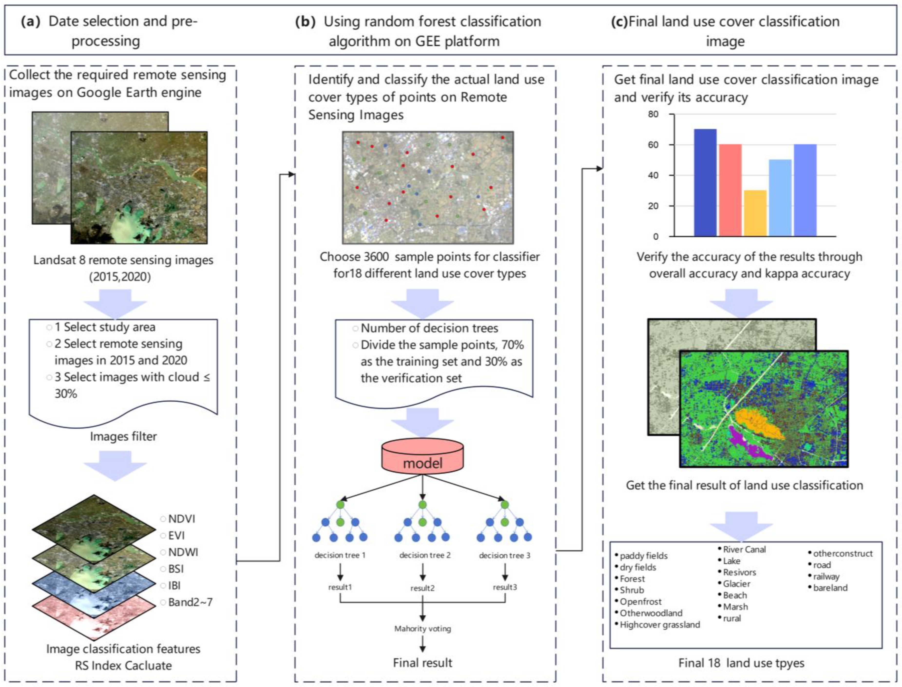
2.3. Land Classification Process with the Random Forest Algorithm in GEE

The Google Earth Engine (GEE) platform is a cloud-based platform dedicated to Earth science data and analytical applications. It offers a wealth of Earth science datasets, including remote sensing imagery and climate and weather data sets. GEE supports data processing and analysis using at least JavaScript 8 and Python3.6’s syntax [26].

Within the study area, approximately 3600 sampling points (SPs) were randomly collected from the periods of 2015 and 2020 as reference data. The Random Forest algorithm was employed to classify land cover types based on these SPs and Landsat-8 SR remote sensing imageries of 2015 and 2020, and the remote sensing features were utilized in the process of classification, including NDVI (Normalized Difference Vegetation Index), EVI (Enhanced Vegetation Index), NDWI (Normalized Difference Water Index), BSI (Bare Soil Index), IBI (Index-Based Biophysical Index), and bands 2 to 7. The SPs were randomly allocated to two datasets for the training and validation sets for the Random Forest algorithm. The training set contained approximately 2520 samples (70%), and the validation set contained 1080 samples (30%). Within the SPs, 18 land use categories were classified, as shown in Figure 2, including paddy fields, dry fields, forest land, shrubs, open forest land, other forest land, high-coverage grassland, channels, reservoirs, lakes, mudflats, wetlands, urban built-up areas, rural settlements, industrial and mining land, highway land, railway land, and bare land. The final classification results were validated using a confusion matrix, and the validation results include the Overall Accuracy (OA) and Kappa coefficient (Kappa). The OA and Kappa for 2015 and 2020 were 86.7%, 83.4%, and 90.3%, 88.1%, respectively. This result validates the model’s effectiveness [27,28] (Figure 2). The final result is the 30 M precision land use and land cover (LULC) maps in 2015 and 2020. Considering the total area of the Suzhou–Wuxi–Changzhou metropolitan area, 30 M precision LULC data can provide sufficient spatial resolution to capture finer landscape features such as patch size, shape, and distribution, as well as accurate distribution of different land use types for calculating ESV distribution. And compared with 10 M precision, 30 M precision reduces the complexity of data processing while maintaining sufficient details, making the evaluation work more efficient and the results more reliable.

Based on the land classification results derived from the Random Forest (RF) algorithm of the Google Earth Engine (GEE) platform, the composition of main land use in the Suzhou–Wuxi–Changzhou metropolitan area in 2020 was as follows: paddy fields 38.7%, dry fields 6.7%, forest land 4.6%, canals 4.8%, lakes 15.3%, reservoirs 1.1%, urban built-up areas 11.8%, rural settlements 5.2%, industrial and mining land 6.8%, highways 4.5%, and railways 0.1%. The main land use composition in 2015 was as follows: paddy fields 38.4%, dry fields 7.9%, forest land 4.7%, canals 6.3%, lakes 13.3%, reservoirs 1.4%, urban built-up areas 12.4%, rural settlements 4.4%, industrial and mining land 5.9%, highways 2.4%, and railways 0.1%. (Figure 1). Over the five-year study period, the area of agricultural land decreased by 0.93%, the area of forest land decreased by 0.10%, and the water body area decreased by 2.32%, while the impervious areas such as urban built-up areas, rural settlements, and industrial and mining land increased by 3.29%.

3. Methods

3.1. inVEST Index Calculation

The inVEST model has strong accuracy in calculating individual ESV indicators. Its modular structure allows researchers to choose appropriate assessment modules based on the characteristics of specific research areas [29]. The regulating and supporting ESVs included in the current inVEST module mainly include annual water yield, carbon storage, habitat quality, sediment delivery ratio, and nutrient delivery ratio.

(1)

Habitat Quality

Habitat quality is calculated by analyzing land use and land cover (LULC) maps and threat levels to habitats. By inputting LULC maps, habitat sensitivity scales, threat source scales, and their distribution data, habitat quality can be evaluated. The calculation results range from 0 to 1, with a higher value indicating a stronger ability to resist disturbance to habitat degradation in the study area. The formula for calculating habitat quality in inVEST is as follows [30,31]:

$$Q_{xj}=H_j\left(1-\left({\displaystyle \frac{D_{xj}^z}{D_{xj}^z-k^z}}\right)\right)$$

(1)

In Formula (1), Q_xj represents the habitat quality of grid x in land use type j; H_j represents the habitat suitability of land use type J; D_xj represents the level of stress on grid x in land use type j; and Z represents the normalization constant; and k is the scaling constant. The formula for calculating D_xj is as follows:

$$D_{xj}={\displaystyle \sum _{r=1}^R{\displaystyle \sum _{y=1}^{Y_r}\left(\frac{W_r}{{\displaystyle \sum _{r=1}^R{W}_r}}\right)}}•r_j{i}_{rxy}{\beta }_x{S}_{jr}$$

(2)

In Formula (2), R is the number of stress factors; r is the stress factor; y is the number of grids for stress factor r; Y_r is the number of grids occupied by stress factors; W_r is the weight of stress factors, with a value range of 0–1; i_rxy is the impact of stress factor r on each grid of the habitat (exponential or linear); β_x is the level of habitat resistance to interference; and S_jr is the relative sensitivity of different habitats to each stress factor.

(2)

Annual Water Yield

The annual water yield module is based on the Budyko water–heat coupling equilibrium hypothesis, and annual average precipitation data [32,33] are required for calculation. The annual water production Y(x) for each grid cell x in the study area is calculated based on the following formula:

$$Y\left(x\right)=\left(1-{\displaystyle \frac{AET\left(x\right)}{P\left(x\right)}}\right)•P\left(x\right)$$

(3)

In Equation (3), AET(x) represents the annual actual evaporation of grid cell x, and P(x) represents the annual precipitation of grid cell x.

(3)

Carbon Storage

The carbon storage module relies on four carbon pools, aboveground biomass, underground biomass, soil organic matter, and dead organic matter, and summarizes the carbon stored in these carbon pools based on land use classification [34]. The calculation principle is as follows:

$$C_T=C_a+C_b+C_s+C_d$$

(4)

In Formula (4), C_T represents the total carbon storage (t/hm²), and C_a, C_b, C_s, and C_d represent the aboveground carbon storage, underground carbon storage, soil carbon storage, and dead carbon storage, respectively.

(4)

Sediment Delivery Ratio

The sediment delivery ratio module was used for the calculation of soil retention; the module generates the spatial distribution of sediment yield in the catchment area based on the spatial resolution of the input DEM data. The model first calculates the amount of soil erosion sediment in each grid cell and then calculates the sediment transport ratio (SDR), which is the proportion of sediment reaching the outlet section of the catchment area to the total amount of soil erosion sediment upstream. Then, it calculates the total annual soil erosion amount in the grid cell [35], expressed in ulsei (ton/hectare year), using the following formula:

$$usl{e}_i=R_i•K_i•L{S}_i•C_i•P_i$$

(5)

In Formula (5), R_i represents the precipitation erosivity factor (MJ·mm (ha·hr)⁻¹), K_i represents the soil erodibility factor (ton·ha·hr (MJ·ha·mm)⁻¹), LS_i represents the slope length factor, C_i represents the vegetation coverage and crop management factor, and P_i represents the water and soil conservation measure factor.

(5)

Nutrient Delivery Ratio

The nutrient delivery ratio model was used for the calculation of nitrogen and phosphorus absorption; this module calculates the number of nutrient elements in each pixel, summarizes the nutrient output and retention for each watershed, and then determines the number of pollutants retained on each landscape plot. The model estimates the pollutant output for each plot based on user input–output coefficients [36]. The formula is as follows:

$$AL{V}_x=HS{S}_x•po{l}_x$$

(6)

In Equation (6), ALV_x is the adjusted loading value of pixel x, pol_x is the output coefficient of pixel x, and HSS_x is the hydrological sensitivity score of pixel x.

3.2. Entropy Weight Method (EWM)

The entropy weight method (EWM) is the method this article uses to calculate the total value of regulating and supporting ESVs; this method can determine the weight of each indicator based on the degree of change in the indicator [37,38,39], thus avoiding the influence of human subjectivity on the results and being able to deal with the problem of strong correlation between indicators such as different ESVs. And the EWM can effectively address the issue of high correlation between indicators and is suitable for various types of indicator sets, whether they are economic, social, or ecological indicators. The steps include standardizing the indicators and setting all indicator values between 0 and 1. Since the ESV indicators used in this study are all positive indicators, the calculation formula is as follows:

$$Y_{ij}={\displaystyle \frac{x_{ij}-x_{j\min }}{x_{j\max }-x_{j\min }}}$$

(7)

In Formula (7), Y_ij is the standardized value of x_ij; x_ij is the jth value of the ith indicator; and x_jmax and x_jmin are the maximum and minimum values of the jth indicator.

$$E={\left\{Y_{ij}\right\}}_{m\times n}=\left(\begin{array}{cccc}{x}_{11}& x_{12}& \dots & x_{2n}\\ x_{21}& x_{22}& \dots & x_{2n}\\ \dots & \dots & \dots & \dots \\ x_{m1}& x_{m1}& \dots & x_{mn}\end{array}\right)$$

(8)

In Formula (8), x_ij is the initial value of the ith (i = 1, 2, … m) point of the jth (j = 1, 2, … n) index.

$$E_i=-k{\displaystyle \sum _{i=1}^m{f}_{ij}\ln }{f}_{ij}$$

(9)

In Formula (9), k > 0, k = 1/ln(m), f_ij = $e_{ij}/{\displaystyle {\sum }_{i=1}^m\ln }{f}_{ij}$, e_ij ≥ 0, and f_ij is the proportion of the ith indicator; when f_ij = 0, it means zero probability produces zero information f_ijlnf_ij = 0.

Calculate the difference coefficient H_i of the ith index using the following formula:

$$H_i=1-E_i$$

(10)

For Formula (10), the normalized index difference coefficient is H_i; to calculate index weight w_i, the Formula (11) is

$$w_i=H_i/{\displaystyle \sum _{n=1}^n{H}_i;\left(0\le w_i\le 1\right)},{\displaystyle \sum _{i=1}^n{w}_i=1}$$

(11)

3.3. Feature Importance Calculation Based on Xgboost

Xgboost (eXtreme gradient boosting) is a popular machine learning algorithm that uses a gradient boosting framework to build ensemble learning models. Xgboost has shown excellent performance in many applications, especially when dealing with driving factors’ feature importance screening. This algorithm has the ability to provide feature importance scores, which helps with decision making for model predictions and can consider both the linear and nonlinear relationships between independent and dependent variables [40].

The method of calculating feature importance in Xgboost is mainly based on two indicators:

(1) Feature Coverage: This reflects the frequency of a feature being used in all trees. A feature that is used as a split point in more trees means that it is more important in the model. The formula for calculating feature coverage is as follows:

$$Coveragej={\displaystyle \frac{{\displaystyle \sum i=1^{n}I\left(j,T_i\right)}}{n}}$$

(12)

In Formula (12), I(j,T_i) is an indicator function that indicates whether feature j is used as a split point in decision tree T_i, and n is the number of decision trees.

(2) Feature Gain: This reflects the contribution of features in decision tree splitting. Xgboost measures the gain of features by considering the split gain (SplitGain) at each split point. The formula for calculating feature gain is as follows:

$$Gainj={\displaystyle \frac{{\displaystyle \sum i=1^n\Delta \backslash loss\left(T_i\right)}}{h}}$$

(13)

In Formula (13), Δ\loss(T_i) is the reduction in the objective function after adding the decision tree T_i, and h is the depth of the decision tree.

(3) Feature importance is a comprehensive reflection of feature coverage and feature gain, which can usually be calculated by the following Formula (14):

$${\mathrm{Importance}}_j=Coverag{e}_j\times Gai{n}_j$$

(14)

3.4. PCA-GWR Method

(1)

Principal Component Analysis

Principal Component Analysis (PCA) is a statistical method that transforms a set of potentially correlated variables into a set of linearly uncorrelated variables through orthogonal transformation. This set of variables is called the principal components (PCs). The purpose of PCA used in this article is to extract the most important driving factors, simplify the complexity of data by retaining the maximum variance of the data after dimensionality reduction, and minimize the loss of information [41,42]. The order of the principal components is such that the first principal component explains most of the differences in the data, and each subsequent principal component explains the maximum proportion of change not explained by the previous principal component. The PCA method can be expressed as follows:

$$P{C}_i=l_{1i}{X}_1+l_{2i}{X}_2+\dots +l_{ni}{X}_n$$

(15)

In Formula (15), PC_i is the ith principal component, and l_ij is the loading of the observed variable X_j (i, j = 1, 2, …, n).

(2)

Geographically Weighted Regression

Geographically weighted regression (GWR) is a local regression method used to analyze spatial data. By introducing a kernel function and bandwidth parameter, it solves the problem of assuming global constant parameters in traditional linear regression and can better reflect the local characteristics of different geographical locations [43]. The GWR structure can be represented as follows:

$$Y_i={\beta }_0\left(u_i,v_i\right)+{\displaystyle \sum _{k=1}^p{\beta }_k}\left(u_i,v_i\right)X_{ik}+{\epsilon }_i$$

(16)

In Formula (16), i is the unique identification number of the SPs (i = 1, 2, …, n), Y_i is the dependent variable, X_ik is the kth independent variable, (u_i,v_i) represents the coordinates of the sampling point i, β_k(u_i,v_i) is the regression parameter of the kth predictor variable, and β(u_i,v_i)0 and ε_i represent the regression constant and random error of the site i, respectively. GWR is a function estimation method that obtains the function value of each independent variable at each geographical location i. In this article, a 1000 × 1000 grid is set up in the study area to extract data.

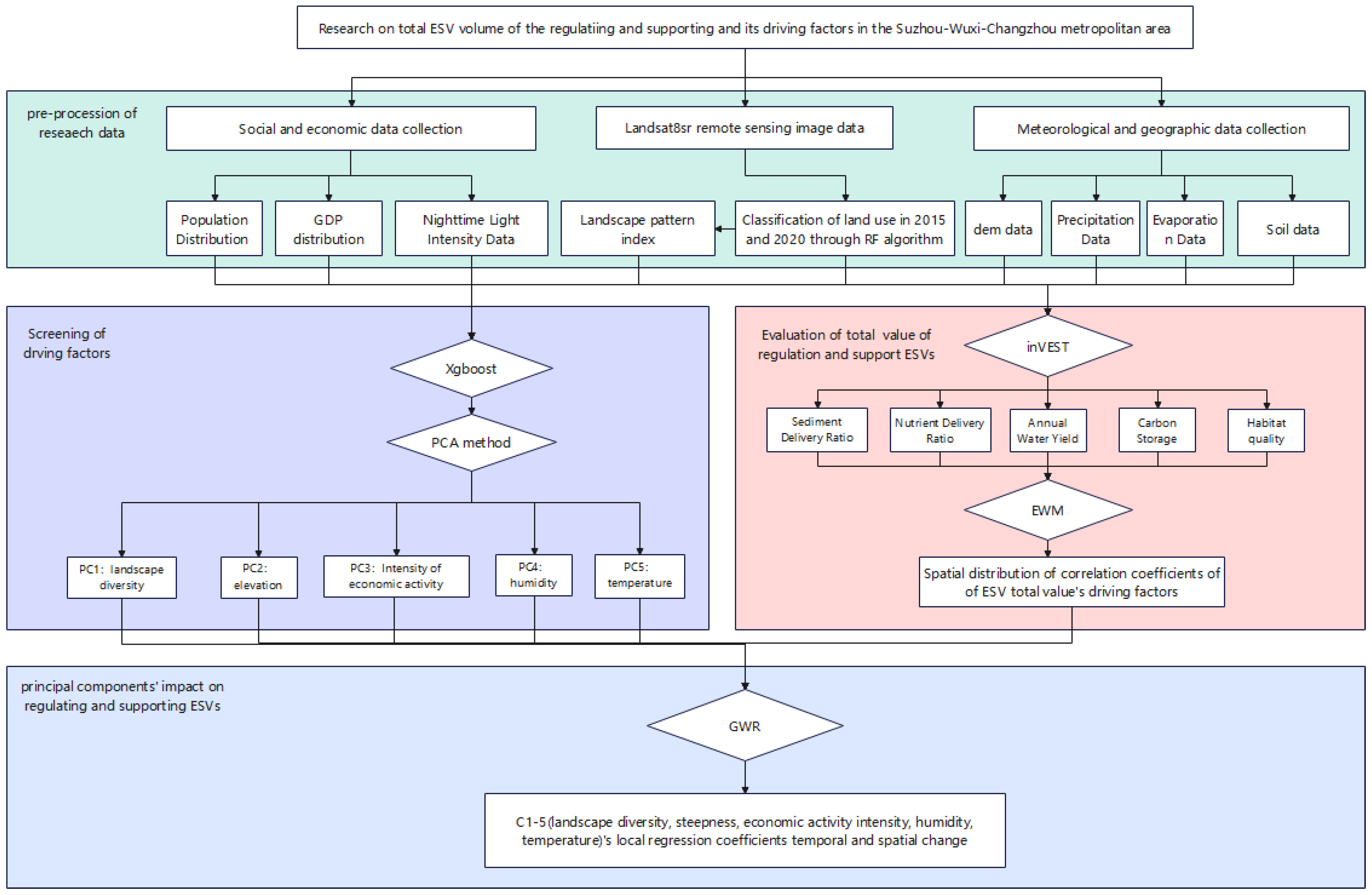
3.5. Overall Workflow

The entire research process in this study includes four steps, including (1) the preprocessing of research data: make a collection of remote sensing, meteorological, economic data for further study, computing the LULC maps of study area in 2015–2020 by RF algorithm; (2) the total value of regulating and supporting ESVs calculation: six ESV indicators calculated by inVEST module, then the weight is allocated to each indicator by EWM and the total value of ESVs in 2015–2020 and its spatial distribution are calculated; (3) driving factors screening: based on the feature importance result of the Xgboost algorithm, the least important factors would be removed first, then PCA is used for dimensionality reduction, transforming numerous factors into several principal components (PCs); and (4) regression model construction: taking principal components (PCs) obtained by PCA as independent variables and taking the total value of ESVs obtained in the second step as dependent variables, and employing geographic weighted regression (GWR) to determine the spatially varying regression coefficients. The workflow is shown in Figure 3.

4. Results

4.1. Entropy Weight Method and ESV Calculation

Before the evaluation of the total value of ESVs and weight assignment, it is necessary to clarify the relationship between different ESV indicators. This paper uses the method of constructing a correlation matrix to calculate the correlation coefficient between ESV indicators and their driving factors. The results are shown in Figure 4. It is evident that there exists a significant correlation not only among different ecosystem service value (ESV) indices but also between these indices and their respective driving factors. Therefore, to address the multicollinearity issue, which leads to unstable results in regression models, we employ the entropy weight method (EWM) and principal component analysis (PCA). These techniques effectively decrease the influence of redundant indicators, preventing the evaluation from being disproportionately influenced by overlapping information and thereby enhancing the rationality of the assessment [44,45].

This article takes six indicators (annual water yield, soil retention, nitrogen and phosphorus absorption, habitat quality, and carbon storage) as regulating and supporting ecosystem services. Using the entropy weight method to obtain the indicators’ weights, the final results are as follows: 0.5% for annual water yield, 56.5% for soil retention, 3.7% for phosphorus absorption, 12.8% for nitrogen absorption, 22.4% for habitat quality, and 4.1% for carbon storage. And the spatial distribution of ESVs in 2015 and 2020 can be obtained.

According to the total value of the ESV distribution maps obtained (Figure 5), in 2015, the minimum was 1.29, the maximum value was 205.44, and the average was 15.21, with a standard deviation of 15.98. In 2020, the minimum value was 5.43, the maximum was 154.54, and the average was 15.17, with a standard deviation of 15.21. The total value of ESVs did not change significantly during the study period, but in terms of spatial distribution, the spatial high and low values of ESVs in 2020 were more clustered. This means that the ESVs are more unevenly distributed geographically. And the spatial autocorrelation of Moran’s index can further confirm it; Moran’s index of ESVs in 2020 was 0.506, and Moran’s index of ESVs in 2015 was 0.476. The closer the Moran’s I index is to 1, the stronger the aggregation of spatial value and the more unevenly distributed [46].

4.2. Xgboost‘s Feature Importance and PCA Results

In the feature importance calculation procession of the Xgboost algorithm, driving factors that do not exhibit a significant impact on the total value of ESVs are automatically removed. In this article, when constructing the Xgboost model, we set the maximum decision tree depth to 4, the learning rate to 0.3, and the number of iterations to 50. Finally, we removed the six least important driving factors, including NP, Mesh, Lsi, Division, Ai, and Runoff. The final reserved driving factor results are shown in

Table 2. Screening results of the characteristic importance of ESV driving factors.

Number	Feature	Gain	Frequency
1	Slope	0.9325973	0.226950355
2	Precipitation	0.018241357	0.056737589
3	Elevation	0.006863327	0.106382979
4	Nighttime light intensity	0.005595812	0.04964539
5	NDVI	0.003815582	0.042553191
6	Evaporation	0.003616705	0.056737589
7	Pladj	0.003088649	0.035460993
8	Humdity	0.003008886	0.021276596
9	LAI	0.002860898	0.035460993
10	PD	0.002483203	0.028368794
11	SIDI	0.00222751	0.021276596
12	SHDI	0.001854396	0.021276596
13	SIEI	0.001833174	0.056737589
14	COHESION	0.001828662	0.014184397
15	GDP	0.001471127	0.035460993
16	NPP	0.001460269	0.042553191
17	LST	0.001158324	0.014184397
18	CONTAG	0.001124751	0.007092199
19	IJI	0.001109848	0.042553191
20	POP	0.001096677	0.021276596
21	Split	0.000791577	0.014184397
22	Wind speed	0.000759522	0.021276596
23	SHEI	0.00069829	0.021276596
24	LPI	0.000414157	0.007092199

.

Following the screening of driving factors using the Xgboost algorithm, a residual collinearity issue persisted among the 24 retained factors. To mitigate this, principal component analysis (PCA) was employed for further dimensionality reduction, transforming retained driving factors into a smaller set of principal components (PCs). PCA analysis resulted in the extraction of five PCs, which collectively accounted for 81.314% of the initial explanatory variable variance (refer to

Table 3. Principal component analysis results of driving factors.

Total Variance Explained
Component	Initial Eigenvalues			Extraction Sums of Squared Loadings
	Total	%of Variance	Cumulative%	Total	%of Variance	Cumulative%
1	11.833	49.306	49.306	11.833	49.306	49.306
2	2.187	9.111	58.417	2.187	9.111	65.417
3	1.700	7.082	65.499	1.700	7.082	72.499
4	1.335	5.563	71.063	1.335	5.563	77.063
5	1.260	5.252	76.314	1.260	5.252	81.314

). The validity of the PCA results was confirmed by successfully passing Bartlett’s test of sphericity.

According to the types of driving factors that constitute each principal component (PC) and their loading sizes, the PCs are named from C1 to C5 (refer to

Table 4. Loading of main components of driving factors.

Component Matrix
Factors	Component
	1	2	3	4	5
Slope	−0.439	0.563	0.168	0.500	0.047
Precipitation	−0.400	0.504	−0.332	−0.261	−0.098
Elevation	−0.539	0.617	0.184	0.406	−0.004
Nighttime light intensity	0.654	0.064	0.294	0.291	0.015
NDVI	−0.576	−0.039	−0.014	−0.104	0.349
Evaporation	−0.746	0.002	−0.061	−0.013	0.335
Pladj	−0.875	−0.010	0.086	0.215	−0.258
Humidity	0.110	−0.604	−0.190	0.634	−0.058
LFI	−0.604	0.393	−0.245	0.203	0.119
PD	0.891	0.112	−0.014	−0.152	0.225
SIDI	0.905	0.107	−0.283	0.053	−0.066
SHDI	0.901	0.116	−0.273	0.067	−0.064
COHESION	−0.850	−0.297	−0.070	−0.108	−0.225
GDP	0.557	0.092	0.641	−0.163	0.066
LST	0.229	−0.346	−0.236	0.271	0.678
NPP	−0.667	0.031	0.070	−0.149	0.474
CONTAH	−0.923	−0.024	0.080	0.158	−0.193
IJI	0.706	0.169	0.109	−0.015	0.047
POP	0.538	0.054	0.616	−0.042	−0.010
Split	0.713	0.305	0.127	0.121	0.257
Windspeed	0.402	−0.518	0.356	0.191	−0.056
SHEI	0.928	0.050	−0.219	0.027	−0.110
LPI	−0.877	−0.226	0.202	−0.149	0.077
SIEI	0.916	0.090	−0.270	0.042	−0.079

):

(1)

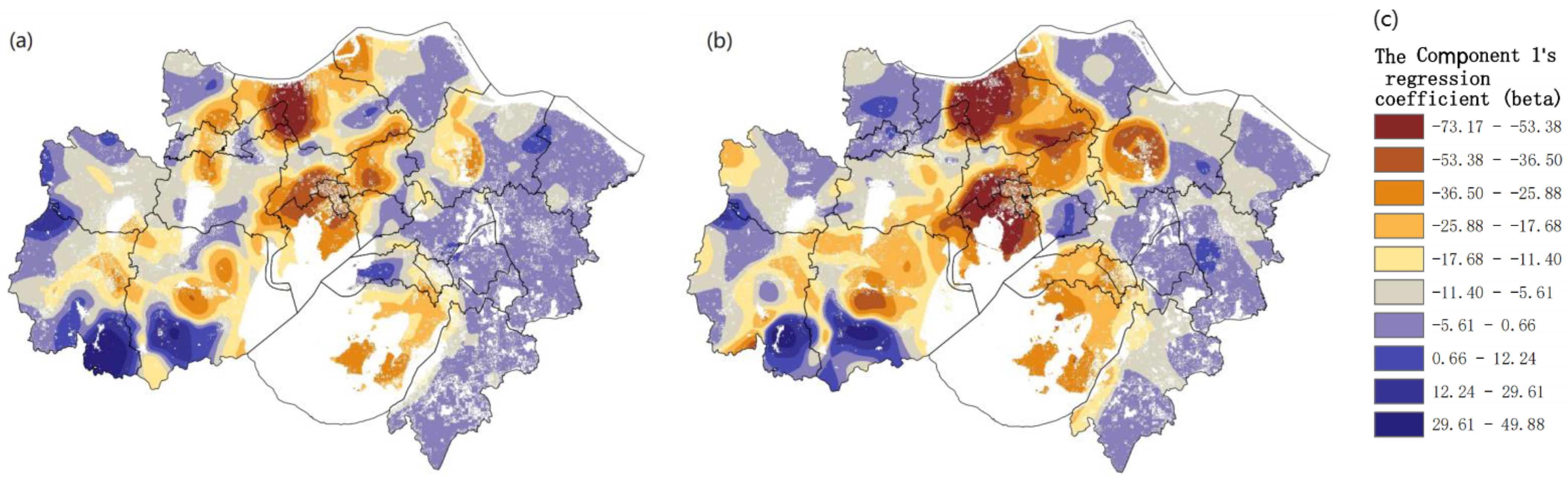
C1 (landscape diversity): With prominent loadings, including Shannon’s evenness index (SHEI = 0.98), Simpson’s diversity index (SIDI = 0.905), and Shannon’s diversity index (SHDI = 0.901), along with a negative loading for contagion index (CONTAG = −0.923), these driving factors capture the highest absolute values and are all indicators of the landscape’s aggregation metrics. Hence, C1 primarily represents landscape diversity.

(2)

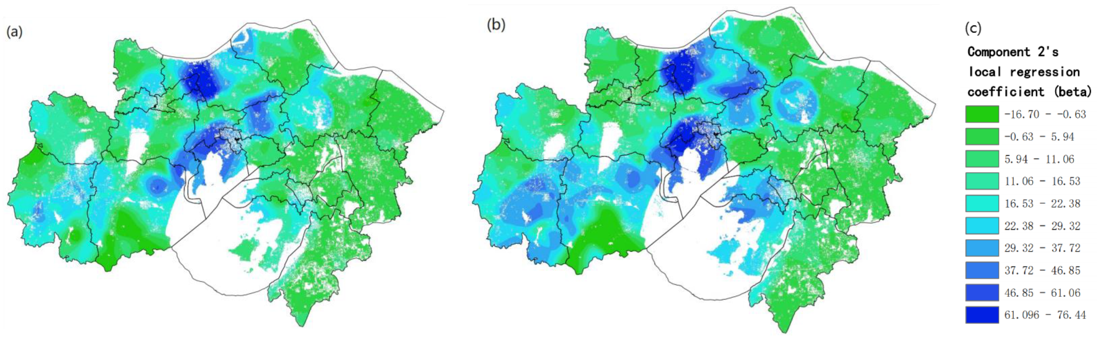
C2 (topographic gradient): With prominent loadings, including elevation (elevation = 0.617), slope (slope = 0.563), and humidity (humidity = −0.694), these driving factors capture the highest absolute values; the elevation and slope are both indicators of the terrain metrics. C2 primarily represents the topographic gradient.

(3)

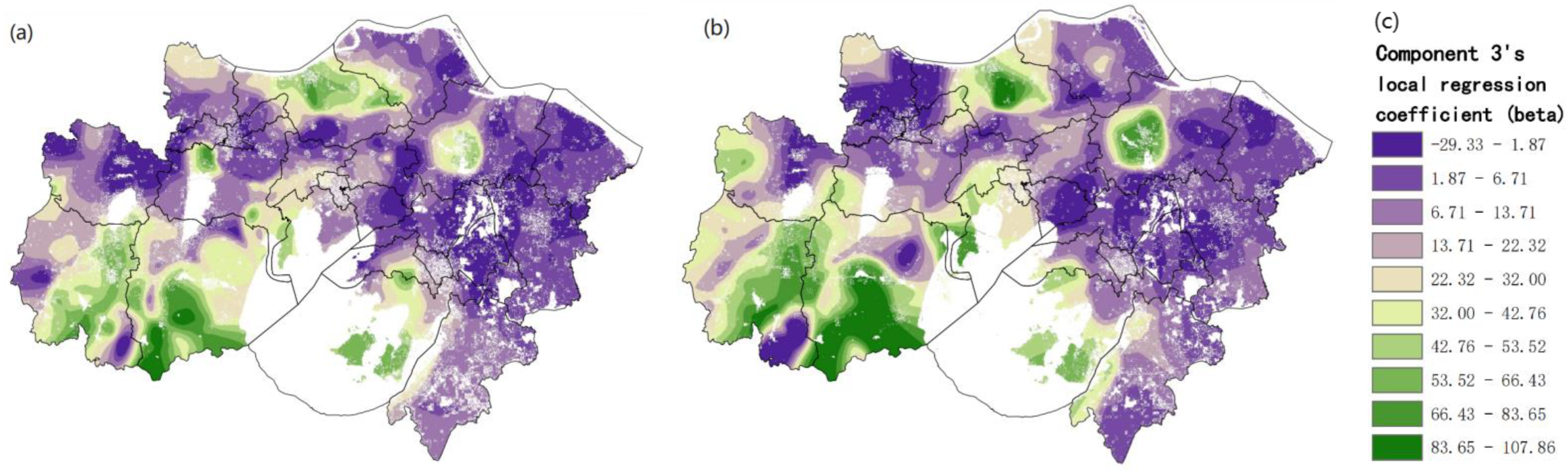
C3 (economic activity intensity): With prominent loadings, including gross domestic product value (GDP = 0.641) and population density (pop = 0.616), these driving factors capture the highest absolute values; the GDP and pop are both indicators of the economic metrics. C3 primarily represents economic activity intensity.

(4)

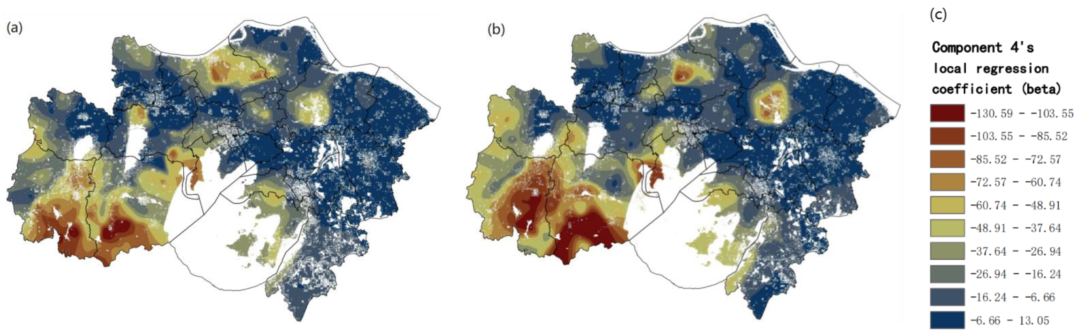
C4 (humidity): In this PC, the humidity is the driving factor with prominent loading (humidity = 0.634); therefore, C4 primarily represents humidity.

(5)

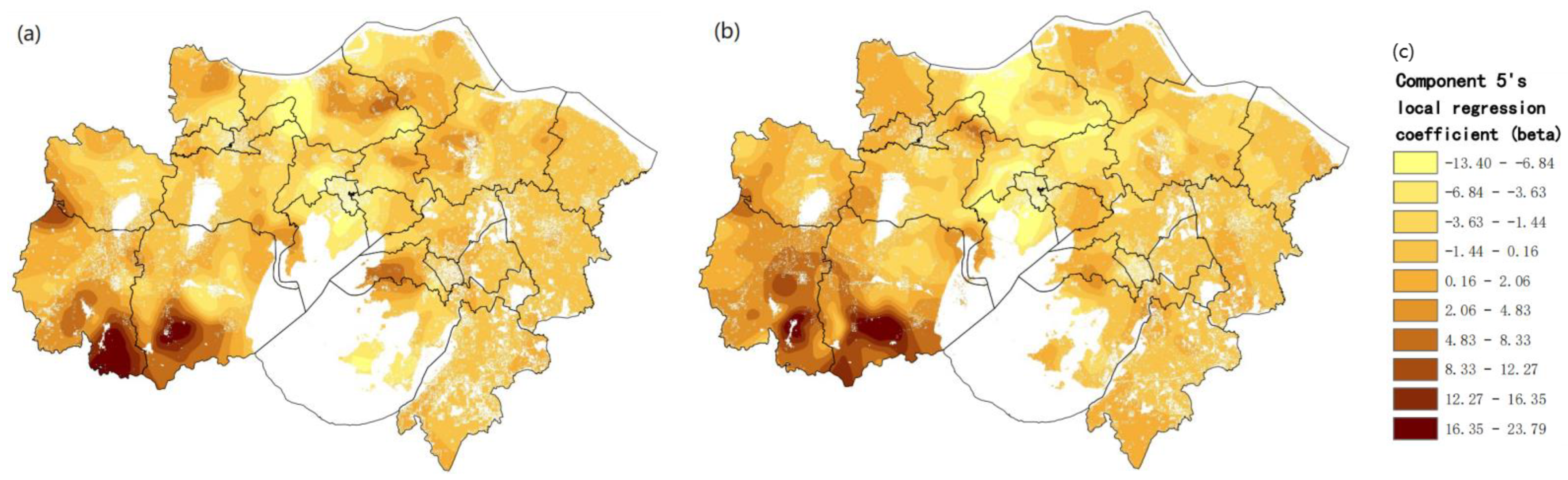
C5 (surface temperature): In this PC, the land surface temperature is the driving factor with prominent loading (LST = 0.678); therefore, C4 primarily represents surface temperature.

4.3. PCA-GWR Fitting Results

To illustrate the comparative fitting merits of the PCA-GWR model, separate models were established using ordinary least squares (OLS) and geographically weighted regression (GWR). These models incorporate five principal components (C1–C5) derived from the principal component analysis (PCA) as independent variables, with the total value of ecosystem service values (ESVs) obtained via the entropy weight method (EWM), serving as the dependent variable. Prior to applying GWR, the global Moran’s index was employed to assess spatial autocorrelation among these principal components. GWR implementation would be unwarranted if no spatial autocorrelation was detected, as OLS would suffice. This study confirmed spatial dependence for all five principal components, thereby validating the use of GWR (

Table 5. Analysis of the global autocorrelation index of the principal components.

Principal Components	Meaning	Moran’s I		Z-Value		p-Value
		2015	2020	2015	2020	2015	2020
C1	landscape diversity	0.711	0.734	256.800	229.993	0.000	0.000
C2	topographic gradient	0.698	0.728	252.199	227.970	0.000	0.000
C3	economic activity intensity	0.708	0.732	255.739	229.252	0.000	0.000
C4	humidity	0.709	0.734	256.165	229.874	0.000	0.000
C5	surface temperature	0.707	0.735	255.432	230.233	0.000	0.000

presents the spatial autocorrelation results).

Finally, we conducted a comparison of the fitting parameters from two models. We compared the models based on their goodness of fit (R²) and the adjusted Akaike Information Criterion (AICc). R² is a value that measures the fitness of the model and reflects the relationship between each driving factor through calculation. By comparing the predicted values and observed values of each regression point, a higher R² value indicates a better fit of the model to the data, reflecting stronger predictive capability. AICc serves as a criterion for model selection, with lower values suggesting a model that explains the data more efficiently, aligning closer with the observed data. The final results show R² of the GWR method in 2015 was 0.788, higher than that of the OLS method (0.546), and the AICc value in 2015 was 12,165, lower than that of the OLS method (17,509). The R² of the GWR method in 2020 was 0.759, higher than that of the OLS method (0.577), and the AICc value was 13,752 in 2020, lower than that of the OLS method (17,768). Based on this comparison, the GWR model demonstrates significantly superior fitting performance over the OLS model, as indicated by higher R² and lower AICc values.

5. Discussion

5.1. C1 and Total Value of ESVs

After the GWR analysis, the temporal and spatial distribution of the principal components’ (PCs) local regression coefficients were presented in Figure 6, Figure 7, Figure 8, Figure 9 and Figure 10, which indicate the impact of the five PCs on the total value of regulating and supporting ESVs. In this paper, different colors are used to represent the degree of different local regression coefficients.

The principal component 1 (C1) represents landscape diversity (Figure 6). The larger the C1 value, the more landscape types, the more evenly distributed the landscape types, and the lower the degree of aggregation within a unit area. From a spatial perspective, C1 mainly has a negative impact on the total value of ESVs in most areas, with only a few areas showing a positive impact. The positive impact areas are mainly southwestern parts of the study area, including southern Liyang District and northwestern and southern Yixing District. The land use in these regions is mainly forest land, which accounts for a large proportion and is densely clustered. The high negative impact areas are mainly central, northern, and lesser southwestern parts of the study area, including Binhu District, Huishan District, and Jiangyin District. These regions are dominated by urban built-up areas and interspersed with little green spaces, such as forest land and paddy fields. From a temporal perspective, the average local regression coefficient in 2015 was −9.8, and in 2020, it was −13.5. And the positive impact area of C1 has significantly shrunk in 5 years, while the negative impact area has significantly expanded.

According to previous research results, the higher the C1, the more landscape types and the more dispersed distribution within a unit area. The increased patches may promote species diversity, but at the same time, the increased edge effect may be detrimental to sensitive species and affect their survival and reproduction, leaving a negative impact on ESVs [47]. And C1 has a negative impact in most areas of the study area. This result is consistent with previous research findings. However, in the areas that have large areas of forest land clustered, evenly distributed, and concentrated, C1 shows a positive impact, which is contrary to the results of general research. In fact, these habitats would not be easily affected by threat sources; an appropriate increase in C1 in these areas means an appropriate increase in biodiversity, which can improve the ability of these areas’ ecosystems to resist disturbance, promote soil retention and nutrients cycling, and enhance soil resistance to erosion. However, when C1 increases beyond a certain level, the resulting biodiversity may no longer promote the total value of ESVs; on the contrary, it may reduce the total value of ESVs due to increased competition and disturbance for resources [48]. The reduction in positive impact areas and the expansion of negative impact areas of C1 indicate that impervious areas are increasing, while habitat areas such as forest land decrease, which is consistent with land use classification results.

5.2. C2 and Total Value of ESVs

Principal component 2 (C2) represents the topographic gradient (Figure 7). A larger C2 value corresponds to higher elevations and slopes, accompanied by lower humidity. From a spatial perspective, C2 has both positive and negative impacts on the total value of ESVs. The positive impact areas are mainly the western, northern, central, and lesser southwestern parts of the study area, including Liyang District, northern Yixing District, Binhu District, Huishan District, Liangxi District, and Jiangyin District. These areas include mainly urban built-up areas and a little farmland, and most of these regions are low-lying areas. The negative impact areas are mainly the northwestern, eastern, and lesser southwestern parts of the study area, including southern and eastern Yixing District, Xinbei District, and most of the Suzhou City area, except Xiangcheng District, Huqiu District, Industrial Park District, and the eastern part of Changshu District; these areas include mainly farmland, forest land, and lesser impervious areas, all with higher elevation. From a temporal perspective, the average local regression coefficient in 2015 was 14.1, and in 2020, it was 16.9. And the positive impact area of C1 expanded significantly over the five studied years, while the negative impact area shrunk significantly.

According to previous research results, when C2 increases, there is an increase in elevation usually, which means an increase in topographic slope that promotes the acceleration of surface runoff and reduces the infiltration time of water on the surface, which may increase the rate of soil erosion, leaving a negative impact on ESVs [49,50,51,52]. And C2 has a negative impact on most areas of study indeed, which is consistent with previous research findings. However, C2 shows a positive impact on the areas dominated by urban built-up areas, which is contrary to the results of general research. The lower the elevation, the more urban low-lying areas will become the collection points of runoff. This will increase the residence time of runoff in these areas and receive more runoff and sediment from upstream. And these impervious surfaces lack vegetation coverage, which will prevent surface runoff from effectively slowing down and infiltrating, resulting in increased soil erosion and runoff scouring of the soil [53]. In addition, impervious surfaces would reduce the potential absorption of nitrogen and phosphorus, allowing more nitrogen and phosphorus to enter urban sewers or nearby water bodies directly with runoff in dissolved or suspended states, thereby reducing the opportunity for natural filtration and absorption in the soil [54]. The increase in the C2 positive impact area reflects the increase in impervious area in these areas, which is consistent with land use classification results.

5.3. C3 and Total Value of ESVs

Principal component 3 (C3) represents the economic activity intensity (Figure 8). C3 has both positive and negative impacts on the total value of ESVs. From a spatial perspective, the positive impact areas are mainly the southwestern and lesser northern and eastern parts of the study area, including southern Liyang District and Yixing District, where forest land in mountainous areas accounts for the largest proportion. The negative impact areas are mainly the northwestern, eastern, and lesser southwestern parts of the study area, including Xinbei District, Jintan District, southern Liyang District, Wuxi’s Xinwu District, Xiangcheng District, Kunshan District, Industrial Park District, Changshu District, and northern Taicang District. These areas are all mainly impervious areas, like urban built-up areas and industrial and mining land. From a temporal perspective, the average local regression coefficient in 2015 was 19.0, and in 2020, it was 23.7. And the positive impact area of C3 expanded significantly over the five years studied.

According to previous research results, higher C3 means growth of GDP and an increase in population; urban built-up areas and industrial and mining areas often would undergo more intense development activities in this case. This process of continuous expansion of impervious areas is always accompanied by changes in the ecological environment and the loss of natural habitats [55]. And economic growth often comes with an increased demand for natural resources, which usually means an increased pressure on the natural environment [56], especially the destruction and fragmentation of habitats, which reduces the total value of ESVs. And C3 indeed leaves a negative impact on ESVs in most areas of the study area; this result is consistent with previous findings. However, in large areas of forest land and a small area of farmland, C3 shows a positive impact on ESVs, which is contrary to general research findings. This phenomenon may be caused in some cases in which forest land areas have used their natural resources to develop industries such as eco-tourism. Such development methods of such industries have increased economic income while protecting the environment [57]. In addition, urbanization and ecological compensation policies may also be employed. As urbanization progresses and population density increases, ecosystem services are threatened, and local governments may take a series of ecological compensation measures to enhance or protect ecological services, and forest land may benefit more from these policies [58]. However, C3 had a significantly negative impact on the forest land in the south of Liyang. The reason is that due to improper economic activities, its landscape of forest land has been cut and fragmented to a much higher degree than other mountainous areas, resulting in the shrinking of habitat patches, reducing the connectivity of the ecosystem and even further affecting the value of water yield and carbon storage. The expansion of the negative impact area of C3 in forest land indicates that the intensity of improper human disturbance to the ecosystem has increased in the five years studied, which is consistent with the results of landscape pattern index calculations that show an increase in landscape fragmentation in this area.

5.4. C4 and Total Value of ESVs

Principal component 4 (C4) represents the humidity (Figure 9). In the overall study area, C4 had a negative impact on the total value of ESVs. From a spatial perspective, the high negative impact areas are mainly southwestern and lesser northern and northeastern parts of the study area, including Liyang District, southern Yixing District, and the southeast corner of Binhu District. The common feature of these areas is that they are all mountainous areas, with a large proportion of forest land. From a temporal perspective, the average local regression coefficient in 2015 was −23.9, and in 2020, it was −27.6. And the high negative impact area of C4 significantly expanded over the five years studied.

According to previous research findings, higher C4 means increased humidity, which may lead to increased soil moisture, reducing the dryness of the soil, which reduces erosion rates to some extent, but increased air humidity also increases soil erosion and reduces water purification capacity by increasing rainfall and rainfall intensity, which can exacerbate soil erosion, especially when rainfall intensity increases and raindrop kinetic energy increases, leading to increased runoff scouring and erosion of soil [59]. And rapid runoff can also carry more pollutants into the water body [60], which would have a negative impact on ESVs. C4 has an overall negative impact on the study area; this result is completely consistent with the previous research findings. And some forest land in mountainous areas with high elevations and steep slopes is more susceptible to rainfall erosion than other areas. The expansion of the C4 high negative impact area and the decrease in the average local regression coefficient represent an increased risk of soil erosion in the Suzhou–Wuxi–Changzhou metropolitan area within the five years studied.

5.5. C5 and Total Value of ESVs

Principal component 5 (C5) represents surface temperature (Figure 10). From a spatial perspective, C5 has both positive and negative impacts on the total value of ESVs; the positive impacts areas are mainly in the southwestern part of the study area, including the southern part of Liyang and Yixing Districts, which are mainly mountainous areas with a large proportion of forest land. The negative impact areas cover most of the study area, except the southwestern part, including northern and central Jiangyin District, Huishan District, Xishan District, Industrial Park District, and Binhu District. From a temporal perspective, the average local regression coefficient in 2015 was 0.09, and in 2020, it was 0.16. The positive impact area of C5 significantly shrunk in the five years studied, while the negative impact area significantly expanded.

According to previous research findings, higher C5 represents higher surface temperature, which can increase soil evaporation and reduce soil moisture, which can affect soil stability and increase potential erosion. In mountainous areas, high vegetation coverage can offset this effect, but in impervious areas like urban built-up areas, this type of impact will intensify. In addition, the increase in surface temperature usually increases evaporation and reduces the retention of surface water, which may affect the ecosystem service of water yield. These reasons can explain why C5 has a negative impact on ESVs of low vegetation coverage areas, such as farmland and impervious areas. On the other hand, moderately high surface temperatures can promote the growth rate of trees, promote carbon storage, and improve habitat quality, thus making C5 have a positive impact on the ESVs of forest land in mountainous areas. This result is consistent with previous research findings. However, the positive impact area of C5 shrunk, and the negative impact area significantly expanded, in the five years studied, showing an increase in impervious area and a decrease in forest area in the study region, which is also consistent with the results of the land use classification calculations.

5.6. Limitations and Future Prospects

This study also has limitations. Firstly, this study is based on the inVEST modules, and the accuracy of the inVEST module highly depends on the quality and completeness of the input data. This results in a research framework that still has the disadvantages of heavy preliminary data preparation and cumbersome steps. Future research should optimize data processing steps with advanced monitoring technologies that can provide more accurate and real-time data and reduce unnecessary steps to improve research efficiency, thereby enhancing the reliability of the results. In addition, such studies mainly start from the scale of cross-regional metropolitan areas. Such studies can well grasp the macrotrend of changes in the entire research area, identify ecological risks in different regions, and help policymakers find the general direction of regional planning. However, when planning needs to be implemented into more specific policy formulation, subsequent research needs to further construct the quantitative relationship between ESVs and driving factors in specific areas of the green space system so as to provide a clearer direction for long-term green space management policies.

6. Conclusions

This study estimated the total value of regulating and supporting ESVs through a combination of EWM and inVEST modules and used the Xgboost algorithm and PCA-GWR methods to overcome the problem of multicollinearity among driving factors, providing a new perspective for the evaluation of multiple ESVs’ total value and the exploration of their driving factors. The results show that (1) landscape diversity, topographic gradient, economic activity intensity, humidity, and surface temperature are the five driving factors that had the greatest impact on the total value of regulating and supporting ESVs, and the increase in impervious area and the decrease in habitat area were the main reasons for the driving factors’ temporal and spatial impact changes in the study area. (2) During the period from 2015 to 2020, the distribution of ESVs in the study area became more clustered and uneven, which may have led to overloading or insufficient ecosystem services in some areas, affecting the health and stability of the natural environment. There is a risk of increased soil erosion throughout the study area, and the mountainous areas in southern Liyang have been significantly negatively affected by human activities; their landscape pattern has become significantly fragmented. This article’s results reveal the ecological problems that have prominently emerged in the Suzhou–Wuxi–Changzhou metropolitan area in the last few years of China’s rapid urbanization, providing a reference for policymakers to maintain regional ecological stability and security. Future research should focus on quantifying the relationship between ESVs and their driving factors in specific areas of green space within the Suzhou–Wuxi–Changzhou metropolitan area to determine the best long-term planning and management policies.

References

1. Han, G.; Yuan, J. The Geographic Area and Spatial Structure of Changchun Metropolitan Area. Sci. Geogr. Sin. 2014, 34, 1202–1209. [Google Scholar]
2. Gao, Y.; Li, J.; Liu, R.; Wang, Z.; Wang, H.; Liu, Y. Temporal and spatial evolution of greenspace system and evaluation of ecosystem services in the core area of the Yangtze River Delta. Chin. J. Ecol. 2020, 39, 956–968. [Google Scholar]
3. Tao, L.; Chen, Y.; Chen, F.; Li, H. Construction of Green Ecological Network in Qingdao (Shandong, China) Based on the Combination of Morphological Spatial Pattern Analysis and Biodiversity Conservation Function Assessment. Sustainability 2023, 15, 16579. [Google Scholar] [CrossRef]
4. Costanza, R.; d’Arge, R.; De Groot, R.; Farber, S.; Grasso, M.; Hannon, B.; Limburg, K.; Naeem, S.; O’neill, R.V.; Paruelo, J. The value of the world’s ecosystem services and natural capital. Nature 1997, 387, 253–260. [Google Scholar] [CrossRef]
5. Xu, K.; Yang, Z. Advances and Prospects in Research of Land Ecosystem Service Value. Asian Agric. Res. 2022, 14, 17–21. [Google Scholar]
6. Sherrouse, B.C.; Semmens, D.J.; Clement, J.M. An application of Social Values for Ecosystem Services (SolVES) to three national forests in Colorado and Wyoming. Ecol. Indic. 2014, 36, 68–79. [Google Scholar] [CrossRef]
7. Yirsaw, E.; Wu, W.; Temesgen, H.; Bekele, B. Effect of temporal land use/land cover changes on ecosystem services value in coastal area of China: The case of Su-Xi-Chang region. Appl. Ecol. Environ. Res. 2016, 14, 409–422. [Google Scholar] [CrossRef]
8. Hamel, P.; Guerry, A.; Polasky, S.; Han, B.; Douglass, J.; Hamann, M.; Janke, B.; Kuiper, J.; Levrel, H.; Liu, H. Mapping the benefits of nature in cities with the InVEST software. npj Urban Sustain. 2021, 1, 25. [Google Scholar] [CrossRef]
9. Sun, Z.; Xue, W.; Kang, D.; Peng, Z. Assessment of Ecosystem Service Values of Urban Wetland: Taking East Lake Scenic Area in Wuhan as an Example. Land 2024, 13, 1013. [Google Scholar] [CrossRef]
10. Wang, J.; Wu, Y.; Gou, A. Habitat quality evolution characteristics and multi-scenario prediction in Shenzhen based on PLUS and InVEST models. Front. Environ. Sci. 2023, 11, 1146347. [Google Scholar] [CrossRef]
11. Wu, Y.; Huang, Z.; Han, D.; Qiu, X.; Pan, Y. Evolution of Urban Ecosystem Service Value and a Scenario Analysis Based on Land Utilization Changes: A Case Study of Hangzhou, China. Sustainability 2023, 15, 8274. [Google Scholar] [CrossRef]
12. Shi, J.; Li, S.; Song, Y.; Zhou, N.; Guo, K.; Bai, J. How socioeconomic factors affect ecosystem service value: Evidence from China. Ecol. Indic. 2022, 145, 109589. [Google Scholar] [CrossRef]
13. Li, W.; Wang, L.; Yang, X.; Liang, T.; Zhang, Q.; Liao, X.; White, J.R.; Rinklebe, J. Interactive influences of meteorological and socioeconomic factors on ecosystem service values in a river basin with different geomorphic features. Sci. Total Environ. 2022, 829, 154595. [Google Scholar] [CrossRef] [PubMed]
14. Chen, C.; Liu, J.; Bi, L. Spatial and temporal changes of habitat quality and its influential factors in China based on the InVEST model. Forests 2023, 14, 374. [Google Scholar] [CrossRef]
15. Xiang, Q.; Kan, A.; Yu, X.; Liu, F.; Huang, H.; Li, W.; Gao, R. Assessment of topographic effect on habitat quality in mountainous area using InVEST Model. Land 2023, 12, 186. [Google Scholar] [CrossRef]
16. Gong, J.; Xie, Y.; Cao, E.; Huang, Q.; Li, H. Integration of InVEST-habitat quality model with landscape pattern indexes to assess mountain plant biodiversity change: A case study of Bailongjiang watershed in Gansu Province. J. Geogr. Sci. 2019, 29, 1193–1210. [Google Scholar] [CrossRef]
17. Guo, R.; Lyu, S.; Feng, J. The Effects of Urban Landscape Pattern Evolution on Habitat Quality Based on InVEST Model: A Case of Harbin City. Int. Rev. Spat. Plan. Sustain. Dev. 2023, 11, 5–25. [Google Scholar] [CrossRef] [PubMed]
18. Benra, F.; De Frutos, A.; Gaglio, M.; Álvarez-Garretón, C.; Felipe-Lucia, M.; Bonn, A. Mapping water ecosystem services: Evaluating InVEST model predictions in data scarce regions. Environ. Model. Softw. 2021, 138, 104982. [Google Scholar] [CrossRef]
19. Guan, X.; Wei, H.; Lu, S.; Dai, Q.; Su, H. Assessment on the urbanization strategy in China: Achievements, challenges and reflections. Habitat Int. 2018, 71, 97–109. [Google Scholar] [CrossRef]
20. Li, Z.; Zhu, J.; Tian, Y. Impact of Land-Use–Land Cover Changes on the Service Value of Urban Ecosystems: Evidence from Chengdu, China. J. Urban Plan. Dev. 2024, 150, 05024028. [Google Scholar] [CrossRef]
21. He, F.; Jin, J.; Zhang, H.; Yuan, L. The change of ecological service value and the promotion mode of ecological function in mountain development using InVEST model. Arab. J. Geosci. 2021, 14, 510. [Google Scholar] [CrossRef]
22. Fangzheng, L.; Danlu, P.; Boya, W. Application of Research on Ecosystem Services in Landscape Planning. Landsc. Archit. Front. 2019, 7, 56–69. [Google Scholar]
23. Li, J.; Luo, G.; Xu, J. Fate and ecological risk assessment of nutrients and metals in sewage sludge from ten wastewater treatment plants in Wuxi City, China. Bull. Environ. Contam. Toxicol. 2019, 102, 259–267. [Google Scholar] [CrossRef]
24. Su, H. Pollution and ecological risk assessment of heavy metal of urban river sediment in Suzhou city. IOP Conf. Ser. Mater. Sci. Eng. 2018, 397, 012073. [Google Scholar] [CrossRef]
25. Chen, L.; Jiang, P.; Chen, W.; Li, M.; Wang, L.; Pian, Y.; Xia, N.; Duan, Y.; Huang, Q. Farmland protection policies and rapid urbanization in China: A case study for Changzhou City. Land Use Policy 2015, 48, 552–566. [Google Scholar]
26. Zhao, Q.; Yu, L.; Li, X.; Peng, D.; Zhang, Y.; Gong, P. Progress and trends in the application of Google Earth and Google Earth Engine. Remote Sens. 2021, 13, 3778. [Google Scholar] [CrossRef]
27. Phan, T.N.; Kuch, V.; Lehnert, L.W. Land cover classification using Google Earth Engine and random forest classifier—The role of image composition. Remote Sens. 2020, 12, 2411. [Google Scholar] [CrossRef]
28. Magidi, J.; Nhamo, L.; Mpandeli, S.; Mabhaudhi, T. Application of the random forest classifier to map irrigated areas using google earth engine. Remote Sens. 2021, 13, 876. [Google Scholar] [CrossRef]
29. Liu, H.; Xiao, W.; Li, Q.; Tian, Y.; Zhu, J. Spatio-temporal change of multiple ecosystem services and their driving factors: A case study in Beijing, China. Forests 2022, 13, 260. [Google Scholar] [CrossRef]
30. Zhong, L.; Wang, J. Evaluation on effect of land consolidation on habitat quality based on InVEST model. Trans. Chin. Soc. Agric. Eng. 2017, 33, 250–255. [Google Scholar]
31. Nematollahi, S.; Fakheran, S.; Kienast, F.; Jafari, A. Application of InVEST habitat quality module in spatially vulnerability assessment of natural habitats (case study: Chaharmahal and Bakhtiari province, Iran). Environ. Monit. Assess. 2020, 192, 487. [Google Scholar] [CrossRef] [PubMed]
32. Redhead, J.; Stratford, C.; Sharps, K.; Jones, L.; Ziv, G.; Clarke, D.; Oliver, T.; Bullock, J. Empirical validation of the InVEST water yield ecosystem service model at a national scale. Sci. Total Environ. 2016, 569, 1418–1426. [Google Scholar] [CrossRef] [PubMed]
33. Yang, X.; Chen, R.; Meadows, M.E.; Ji, G.; Xu, J. Modelling water yield with the InVEST model in a data scarce region of northwest China. Water Supply 2020, 20, 1035–1045. [Google Scholar] [CrossRef]
34. Huang, Z.; Zhao, J.; Xiao, H.; Guo, W.; Yang, Z.; Liu, J. Water service supply and demand situation and driving factors in Shiyang River Basin. J. Soil Water Conserv. 2021, 35, 228–235. [Google Scholar]
35. Zhao, M.; He, Z.; Du, J.; Chen, L.; Lin, P.; Fang, S. Assessing the effects of ecological engineering on carbon storage by linking the CA-Markov and InVEST models. Ecol. Indic. 2019, 98, 29–38. [Google Scholar] [CrossRef]
36. Matomela, N.; Li, T.; Ikhumhen, H.O.; Raimundo Lopes, N.D.; Meng, L. Soil erosion spatio-temporal exploration and Geodetection of driving factors using InVEST-sediment delivery ratio and Geodetector models in Dongsheng, China. Geocarto Int. 2022, 37, 13039–13056. [Google Scholar] [CrossRef]
37. Benez-Secanho, F.J.; Dwivedi, P. Does quantification of ecosystem services depend upon scale (resolution and extent)? A case study using the InVEST nutrient delivery ratio model in Georgia, United States. Environments 2019, 6, 52. [Google Scholar] [CrossRef]
38. Ji, Y.; Huang, G.H.; Sun, W. Risk assessment of hydropower stations through an integrated fuzzy entropy-weight multiple criteria decision making method: A case study of the Xiangxi River. Expert Syst. Appl. 2015, 42, 5380–5389. [Google Scholar] [CrossRef]
39. Wang, Q.; Yuan, X.; Zhang, J.; Gao, Y.; Hong, J.; Zuo, J.; Liu, W. Assessment of the sustainable development capacity with the entropy weight coefficient method. Sustainability 2015, 7, 13542–13563. [Google Scholar] [CrossRef]
40. Wang, G.; Li, P.; Wang, H.; Li, G. Assessments of integrated ecosystems in mining areas based on energy analysis. Acta Ecol. Sin. 2015, 35, 4367–4376. [Google Scholar]
41. Ramraj, S.; Uzir, N.; Sunil, R.; Banerjee, S. Experimenting XGBoost algorithm for prediction and classification of different datasets. Int. J. Control Theory Appl. 2016, 9, 651–662. [Google Scholar]
42. Zhai, L.; Li, S.; Zou, B.; Sang, H.; Fang, X.; Xu, S. An improved geographically weighted regression model for PM2.5 concentration estimation in large areas. Atmos. Environ. 2018, 181, 145–154. [Google Scholar] [CrossRef]
43. Soltanifard, H.; Kashki, A.; Karami, M. Analysis of spatially varying relationships between urban environment factors and land surface temperature in Mashhad city, Iran. Egypt. J. Remote Sens. Space Sci. 2022, 25, 987–999. [Google Scholar] [CrossRef]
44. Wang, S.; Fang, C.; Ma, H.; Wang, Y.; Qin, J. Spatial differences and multi-mechanism of carbon footprint based on GWR model in provincial China. J. Geogr. Sci. 2014, 24, 612–630. [Google Scholar] [CrossRef]
45. Meng, L.; Huang, J.; Dong, J. Assessment of rural ecosystem health and type classification in Jiangsu province, China. Sci. Total Environ. 2018, 615, 1218–1228. [Google Scholar] [CrossRef] [PubMed]
46. Kumar, E.; Subramani, T.; Karunanidhi, D. Integrated approach of ecosystem services for mine reclamation in a clustered mining semi-urban region of South India. Urban Clim. 2022, 45, 101246. [Google Scholar] [CrossRef]
47. Liu, Y.-Q.; Zhang, H.-B.; Zhang, Y.-F. Spatio-temporal variation of ecosystem services value in Yancheng coastal zone. J. Zhejiang AF Univ. 2019, 36, 774–782. [Google Scholar]
48. Peng, Y.; Fan, M.; Qing, F.; Xue, D. Study progresses on effects of landscape metrics on plant diversity. Ecol. Environ. Sci. 2016, 25, 1061–1068. [Google Scholar]
49. Tian, T. The Effect of Landscape Patterns on Avian Communities during Summer Months in Beijing’s Urban Parks. Landsc. Archit. Front. 2016, 4, 10–22. [Google Scholar]
50. Liu, C.; Liu, Y.; Giannetti, B.F.; Almeida, C.M.; Sevegnani, F.; Li, R. Spatiotemporal differentiation and mechanism of anthropogenic factors affecting ecosystem service value in the Urban Agglomeration around Poyang Lake, China. Ecol. Indic. 2023, 154, 110733. [Google Scholar] [CrossRef]
51. Hou, W.; Gao, J. Simulating runoff generation and its spatial correlation with environmental factors in Sancha River Basin: The southern source of the Wujiang River. J. Geogr. Sci. 2019, 29, 432–448. [Google Scholar] [CrossRef]
52. Zhang, S.-B.; Li, J.-G.; Huang, J.-H.; Zhang, W.-T.; Yang, W.-Y.; Wang, F.; Zhang, P.-P. Impact of the Grass Coverage on Runoff and Sediment in the Yili River Valley. Acta Agric. Univ. Jiangxiensis 2016, 38, 995–1001. [Google Scholar]
53. Pan, D.; Qi, L.; Tian, F.; Yuan, X. Improvement of combination weighting-fuzzy clustering algorithm and its application in flood risk assessmen. South-to-North Water Transf. Water Sci. Technol. 2021, 18, 38–56. [Google Scholar]
54. Li, Y.; Wang, D.; Yuan, J.; Liu, X. Temporal and spatial pattern and functional zoning of land use in alpine canyon region based on terrain gradient. Bull. Soil Water Conserv. 2020, 40, 303–311. [Google Scholar]
55. Wang, B.; Yang, T. Value evaluation and driving force analysis of ecosystem services in Yinchuan City from 1980 to 2018. Arid Land Geogr. 2021, 44, 552–564. [Google Scholar]
56. Wu, S.; Ma, S.; Wang, H.; Wang, L.; Jiang, J. Spatiotemporal variations of ecosystem service value in the hill and mountain belt of southern China across different altitude gradients. Chin. J. Ecol. 2023, 42, 966. [Google Scholar]
57. Shasha, Z.T.; Geng, Y.; Sun, H.-p.; Musakwa, W.; Sun, L. Past, current, and future perspectives on eco-tourism: A bibliometric review between 2001 and 2018. Environ. Sci. Pollut. Res. 2020, 27, 23514–23528. [Google Scholar] [CrossRef] [PubMed]
58. Jia, M.Y.; Chen, T. Identifying and Optimizing Hydro-ecological Security Pattern with Land Use Change Modeling: A Case Study of Tianjin. Landsc. Archit. 2021, 28, 95–100. [Google Scholar]
59. Qin, Y.; Cheng, J.; Zhang, H.; Li, Z. A study of the raindrop impact to splash erosion. J. Soil Water Conserv. 2014, 28, 74–78. [Google Scholar]
60. Chen, Z.; Zhu, B.; Tang, J.; Liu, X. Influence of slope gradient on soil erosion in the hilly area of purple soil under natural rainfall. Pearl River 2016, 37, 29–33. [Google Scholar]
Figure 1. Land use map of Suzhou–Wuxi–Changzhou metropolitan area in 2020: (a) Land classification in the Suzhou–Wuxi–Changzhou region with a precision of 30 M and its administrative division. (b) The classification image contains 18 types of land use.
Land 13 01191 g001
Figure 2. Steps and process of Random Forest algorithm on GEE platform, including (a) date selection and preprocessing and (b) using Random Forest classification algorithm on GEE platform (c).
Land 13 01191 g002
Figure 3. Steps and process of this article’s overall workflow.
Land 13 01191 g003
Figure 4. Correlation thermodynamic diagram: (a) Date selection and preprocessing. (b) Using Random Forest classification algorithm on GEE platform.
Land 13 01191 g004
Figure 5. Spatial distribution of regulating and supporting ESVs: (a) The total value of ESVs in 2015. (b) The total value of ESVs in 2020. (c) Measurement table for the total value of ESVs.
Land 13 01191 g005
Figure 6. Local regression coefficient distribution of principal component 1: (a) 2015. (b) 2020. (c) Measurement table for local regression coefficient of C1.
Land 13 01191 g006
Figure 7. Local regression coefficient distribution of principal component 2: (a) 2015. (b) 2020. (c) Measurement table for local regression coefficient of C2.
Land 13 01191 g007
Figure 8. Local regression coefficient distribution of principal component 3: (a) 2015. (b) 2020. (c) Measurement table for local regression coefficient of C3.
Land 13 01191 g008
Figure 9. Local regression coefficient distribution of principal component 4: (a) 2015. (b) 2020. (c) Measurement table for local regression coefficient of C4.
Land 13 01191 g009
Figure 10. Local regression coefficient distribution of principal component 5: (a) 2015. (b) 2020. (c) Measurement table for local regression coefficient of C5.
Land 13 01191 g010