
Integration between Dockless Bike-Sharing and Buses: The Effect of Urban Road Network Characteristics
Abstract
:1. Introduction
2. Literature Review
2.1. Integration of Bikeshare and Public Transport
2.2. Urban Road Network Influencing the Integration of Bikeshare and Public Transport
2.2.1. Analysis of Road Network Characteristics in the Context of Built Environment Effects
2.2.2. Quantifying Road Characteristics in Studies Related to Shared Bicycle Riding Behavior
2.3. Other Factors Influencing the Integration of Bikeshare and Public Transport
3. Method
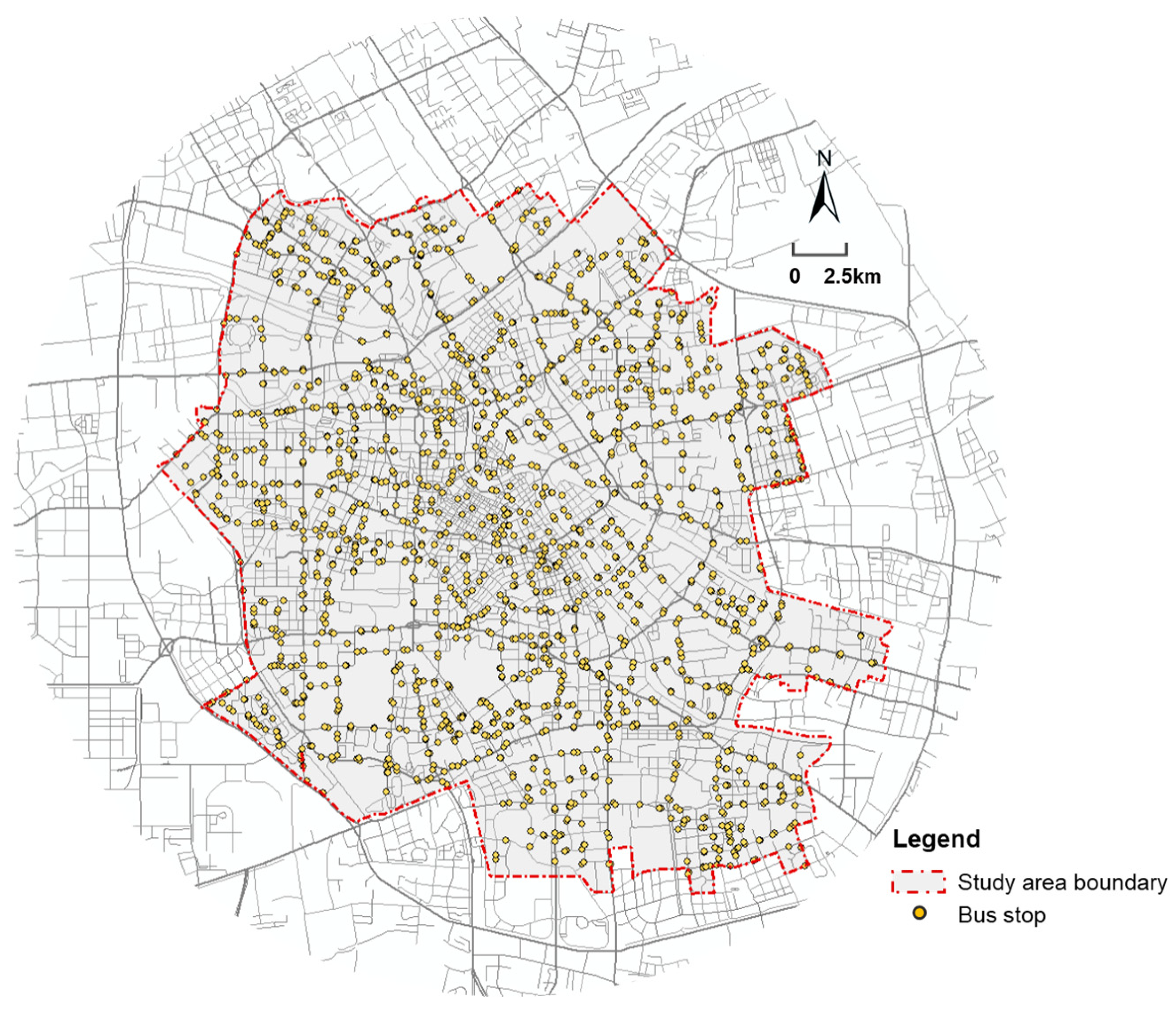
3.1. Study Area
3.2. Data
3.3. Measuring the Variables
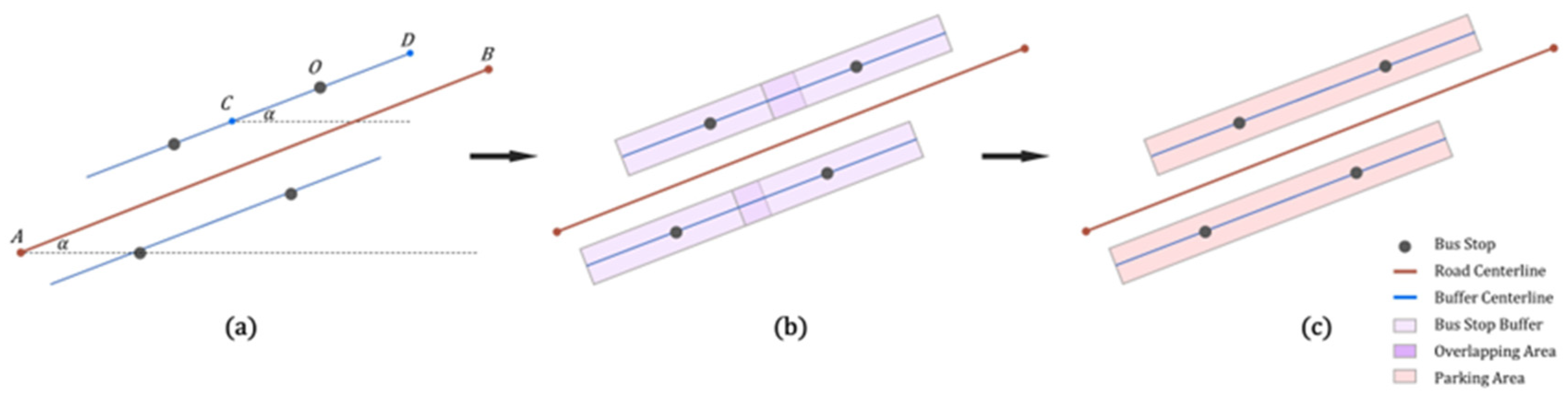
3.3.1. Measure of the DBS–Bus Integrated Use
3.3.2. Measure of Urban Road Network Variables and Control Variables
3.4. Models: Zero-Inflated Negative Binomial Regression (ZINB)
4. Results and Analysis
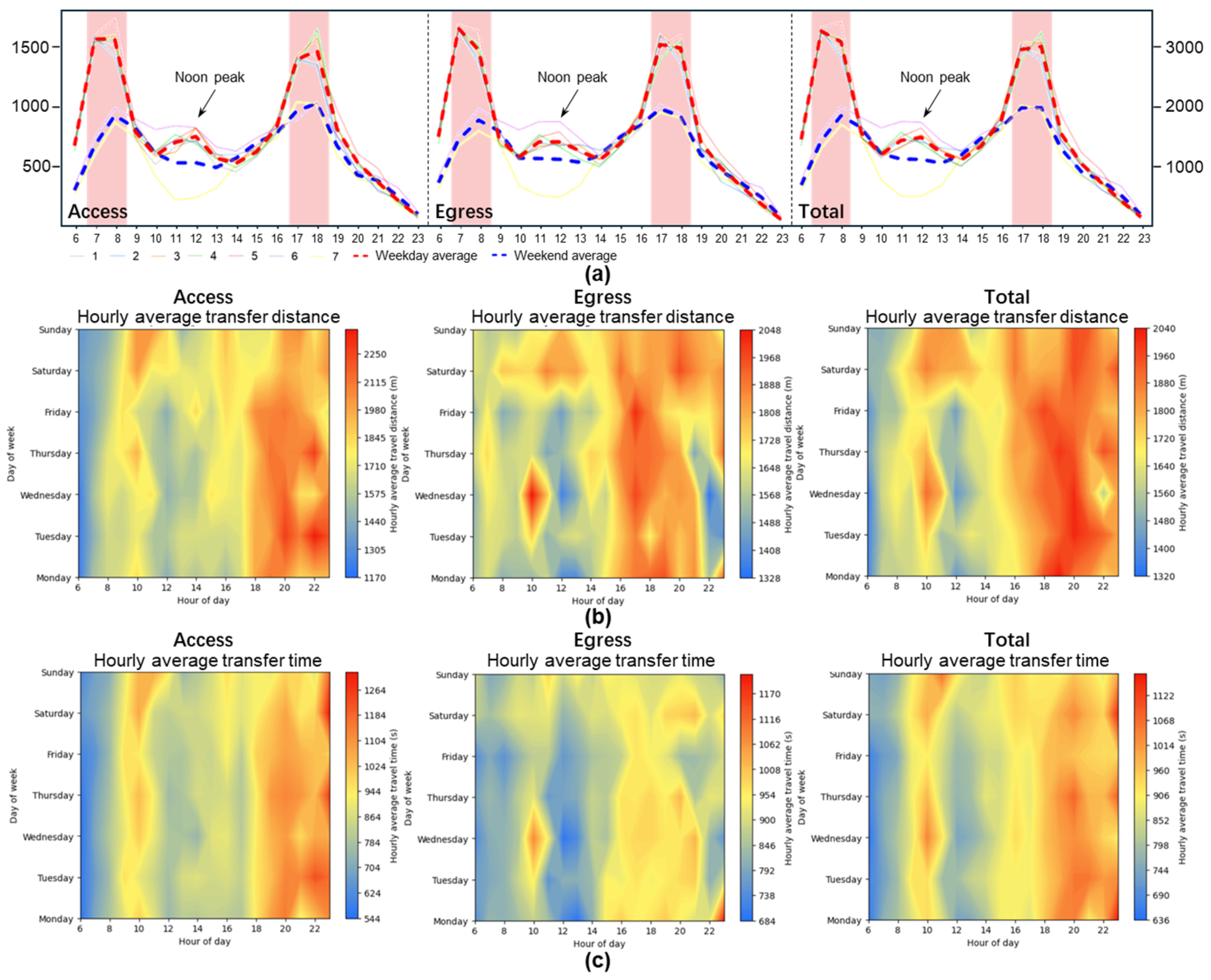
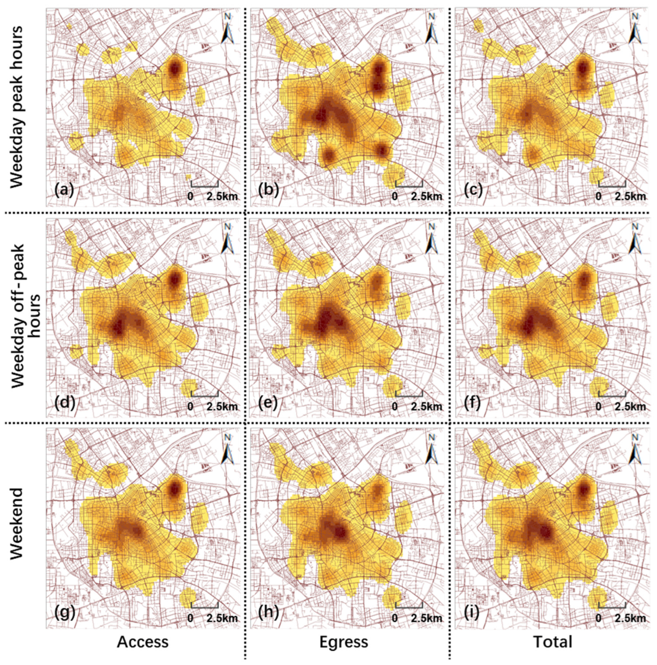
4.1. Spatial and Temporal Dynamic Features of DBS–Bus Integration
4.2. Road Network Characteristics in Tianjin Inner City
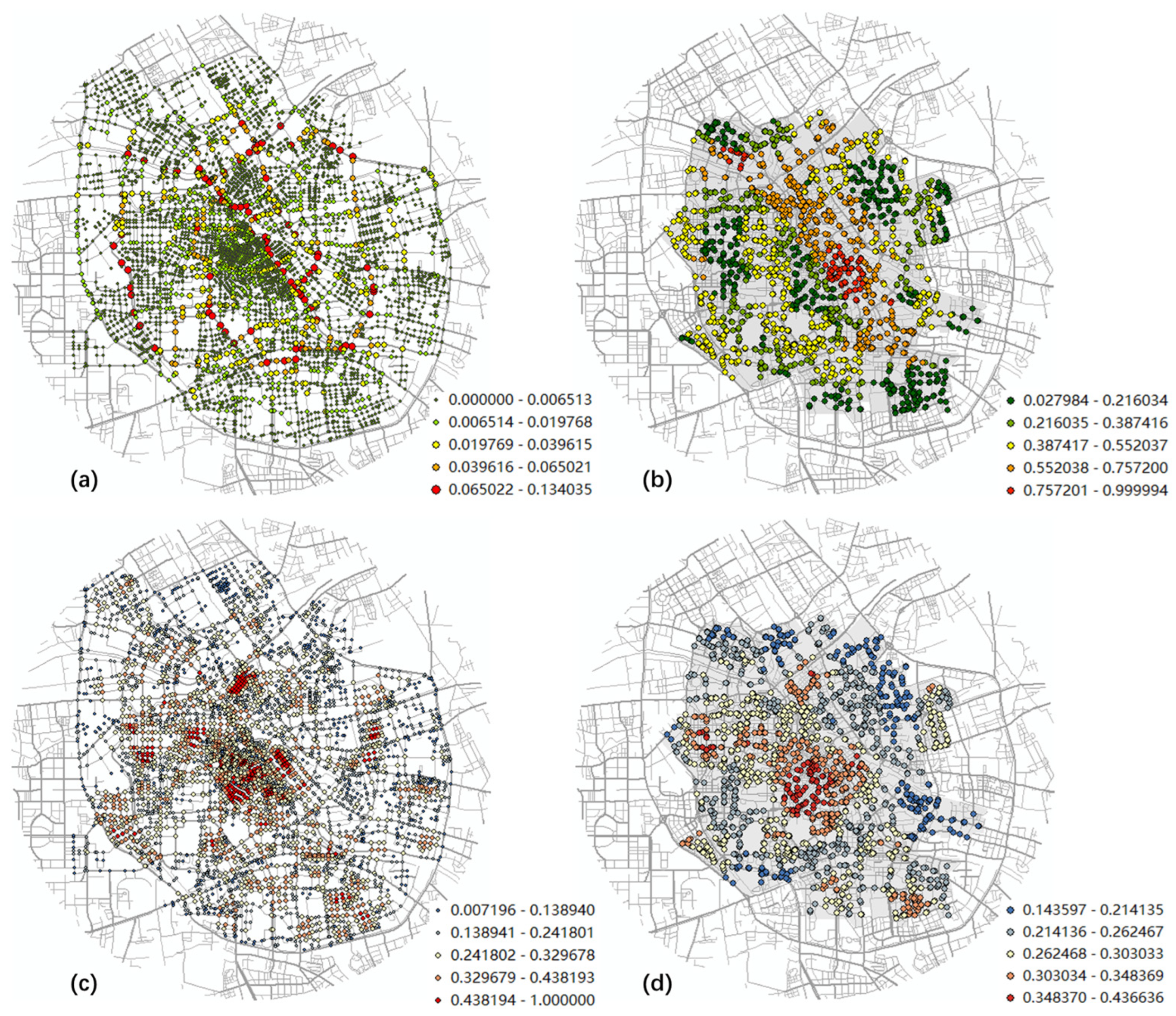
4.2.1. Spatial Distribution Characteristics of Network Centrality
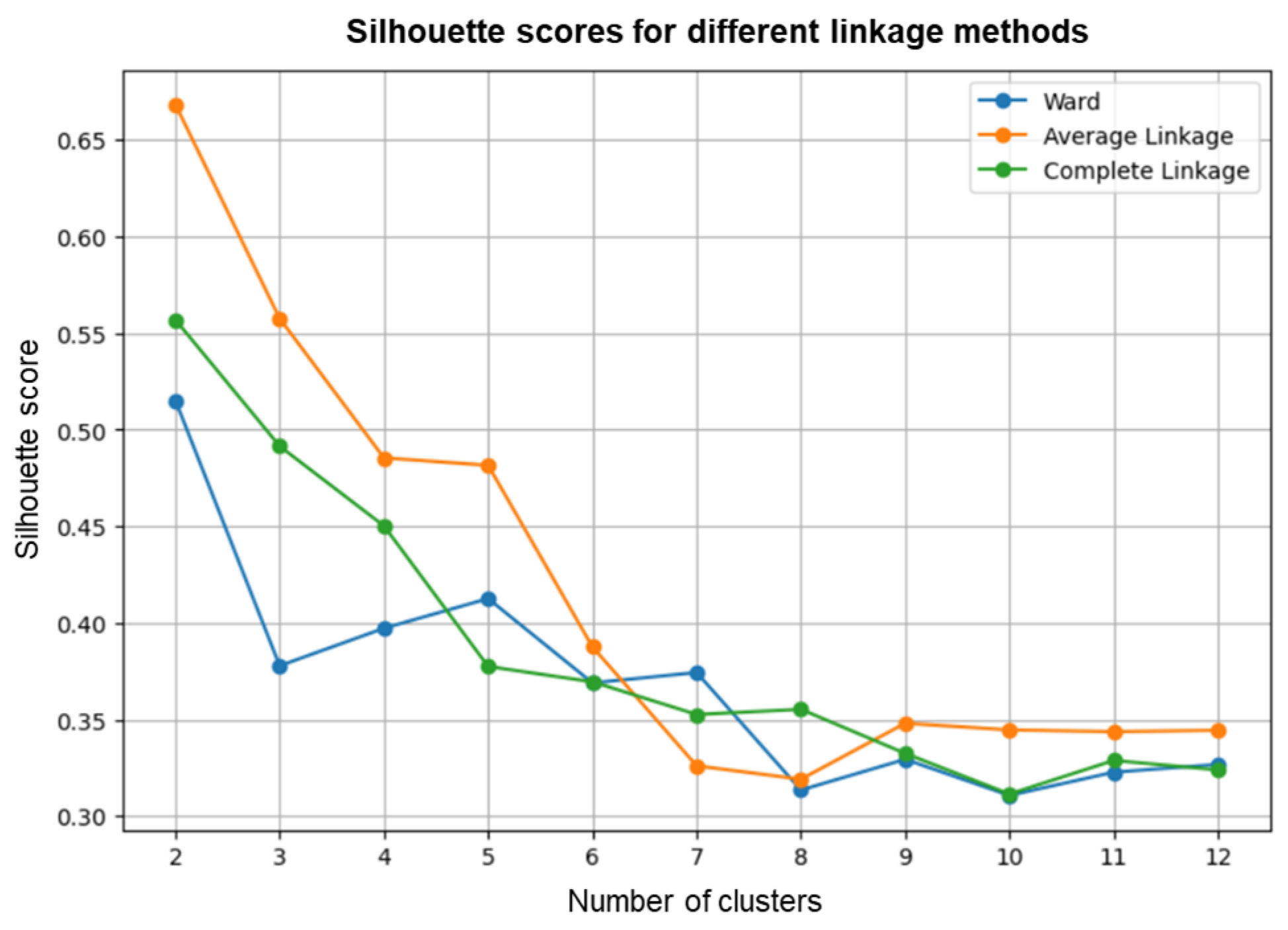
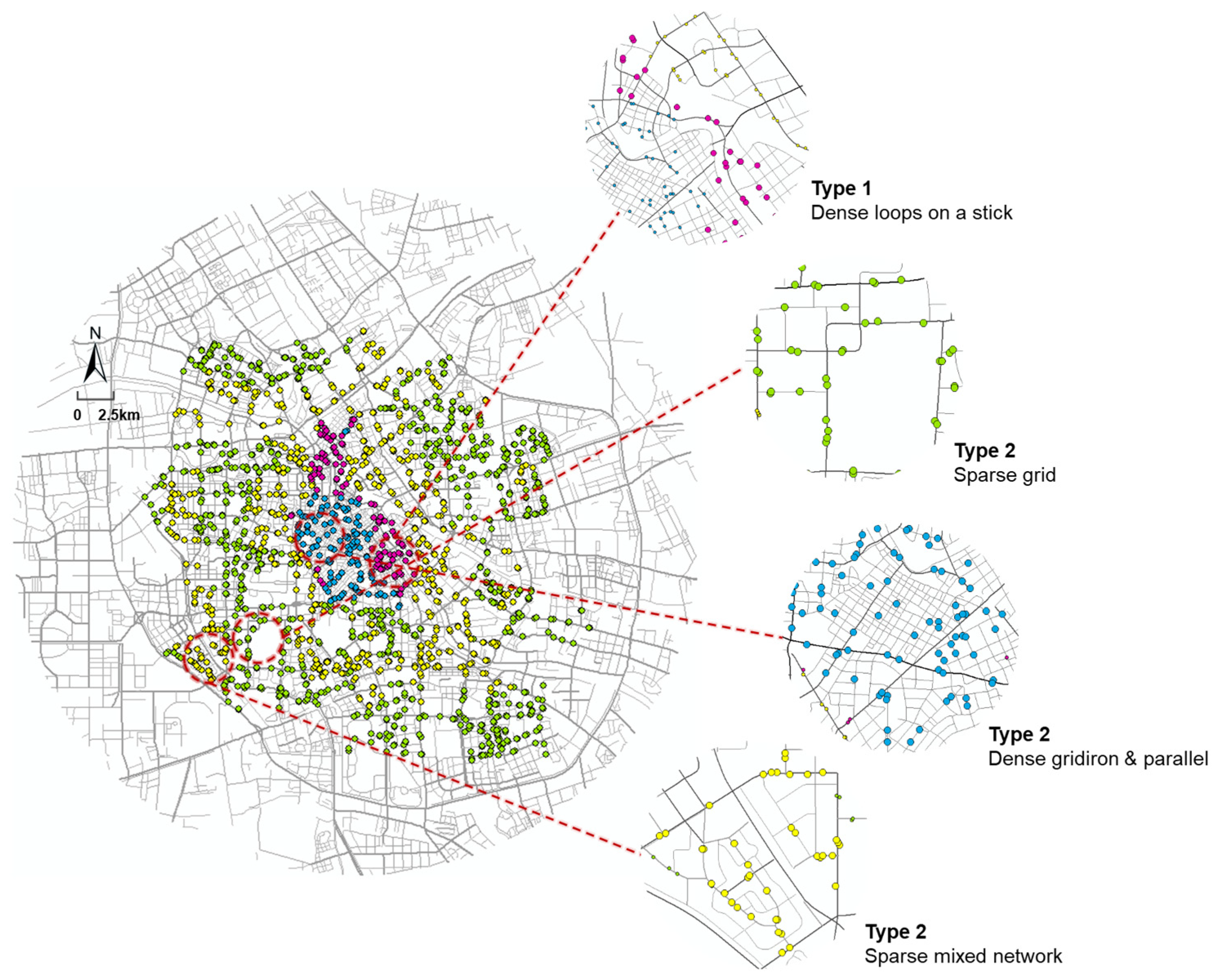
4.2.2. Major Morphometric-Based Street Patterns
- (1)
- Type 1 was identified as the ‘dense loops on a stick’, reflected in the highest betweenness centrality of 0.740. It is a street pattern with smaller blocks affiliated with the artillery road, considering the relatively high value of road density and number of intersections. This type of catchment area is mainly distributed linearly along the banks of the river in the old city center, where many dense road networks form T-junctions with the main roads.
- (2)
- Type 2 was the ‘sparse grid’, as it had the lowest value of all the metrics. Most street junctions in each catchment link four similar roads, connected throughout the network. It is widely distributed in large-scale blocks on the edge of the inner city.
- (3)
- Type 3, ‘dense gridiron and parallel’, is a typical pattern that distinguishes itself from the others with the highest road density and a relatively low centrality. Mostly located in the old city center, it tends to have a nonhierarchical network structure and, thus, provide relatively better connectivity.
- (4)
- Type 4 was the ‘sparse mixed network’, which falls between types 1 and 2. Although it shows a certain degree of regularity and uniformity compared to type 1, it is way less rigid than type 2. This was reflected in the medium average centrality of 0.564, average road density of 6.410, and average intersection number of 48.137.
4.3. Influence of Road Features on DBS–Bus Integration
4.3.1. Different Effects on DBS–Bus Total Integrated Use during Three Time Periods
4.3.2. Different Effects on DBS–Bus Access Integrated Use and Egress Integrated Use

| Variable | Access Integrated Use during Weekday Peak Hours | Egress Integrated Use during Weekday Peak Hours | Total Integrated Use during Weekday Peak Hours | |||||||
|---|---|---|---|---|---|---|---|---|---|---|
| Coef. | Std. | p | Coef. | Std. | p | Coef. | Std. | p | ||
| Count | ||||||||||
| Road features in size | ||||||||||
| Road grade | Secondary road | 0.140 | 0.101 | 0.165 | 0.247 | 0.102 | 0.015 | 0.202 | 0.100 | 0.043 |
| Branch road | 0.239 | 0.111 | 0.031 | 0.144 | 0.112 | 0.199 | 0.188 | 0.109 | 0.085 | |
| Residential road | 0.240 | 0.142 | 0.091 | 0.329 | 0.140 | 0.019 | 0.273 | 0.139 | 0.050 | |
| Major road density | −0.300 | 0.112 | 0.007 | −0.196 | 0.111 | 0.077 | −0.285 | 0.110 | 0.009 | |
| Secondary road density | 0.251 | 0.087 | 0.004 | 0.269 | 0.085 | 0.002 | 0.283 | 0.085 | 0.001 | |
| Branch road density | 0.120 | 0.050 | 0.015 | 0.079 | 0.048 | 0.101 | 0.105 | 0.048 | 0.028 | |
| Road network structure features | ||||||||||
| Betweenness centrality | −0.536 | 0.334 | 0.108 | −0.895 | 0.329 | 0.006 | −0.608 | 0.328 | 0.063 | |
| Eigenvector centrality | −0.021 | 3.029 | 0.994 | −9.173 | 3.033 | 0.002 | −3.584 | 2.998 | 0.232 | |
| Number of 3-legged intersections | 0.007 | 0.005 | 0.128 | 0.000 | 0.005 | 0.951 | 0.004 | 0.005 | 0.412 | |
| Proportion of 3-legged intersections | −0.275 | 1.199 | 0.819 | −2.840 | 1.215 | 0.019 | −1.298 | 1.184 | 0.273 | |
| Number of culs-de-sac | 0.136 | 0.044 | 0.002 | 0.184 | 0.043 | 0.000 | 0.161 | 0.043 | 0.000 | |
| Proportion of culs-de-sac | −2.769 | 2.532 | 0.274 | −11.212 | 2.509 | 0.000 | −6.907 | 2.447 | 0.005 | |
| Categorized street pattern | Type 2 | 0.908 | 0.275 | 0.001 | 0.518 | 0.272 | 0.057 | 0.750 | 0.271 | 0.006 |
| Type 3 | 0.458 | 0.285 | 0.108 | 0.383 | 0.281 | 0.172 | 0.459 | 0.282 | 0.103 | |
| Type 4 | 0.948 | 0.218 | 0.000 | 0.659 | 0.213 | 0.002 | 0.824 | 0.214 | 0.000 | |
| Transport facilities | ||||||||||
| Distance to nearby metro station | 0.290 | 0.114 | 0.011 | 0.088 | 0.113 | 0.437 | 0.232 | 0.113 | 0.041 | |
| Distance to CBD | −0.266 | 0.030 | 0.000 | −0.292 | 0.030 | 0.000 | −0.282 | 0.029 | 0.000 | |
| Transfer distance | −1.499 | 0.168 | 0.000 | −1.170 | 0.200 | 0.000 | −0.852 | 0.102 | 0.000 | |
| _cons | 3.234 | 1.721 | 0.060 | 7.885 | 1.795 | 0.000 | 6.328 | 1.714 | 0.000 | |
| Inflate | ||||||||||
| Residential use density | −0.071 | 0.026 | 0.007 | −0.020 | 0.014 | 0.138 | −0.019 | 0.018 | 0.304 | |
| Company density | 1.900 | 0.643 | 0.003 | 1.459 | 0.803 | 0.069 | 1.623 | 1.134 | 0.152 | |
| Education facility density | −0.165 | 0.055 | 0.003 | −0.425 | 0.211 | 0.044 | −0.521 | 0.325 | 0.109 | |
| Restaurant density | 0.041 | 0.015 | 0.006 | 0.018 | 0.013 | 0.153 | 0.019 | 0.017 | 0.251 | |
| Shopping use density | 0.039 | 0.027 | 0.155 | 0.052 | 0.041 | 0.199 | 0.057 | 0.056 | 0.304 | |
| _cons | 0.873 | 1.951 | 0.655 | 1.098 | 2.792 | 0.694 | 1.383 | 2.824 | 0.624 | |
| Log-likelihood | −5597.734 | −5761.958 | −6780.83 | |||||||
| LR chi2 | 254.38 | 223.33 | 250.66 | |||||||
| Variable | Access Integrated Use during Weekday Off-Peak Hours | Egress Integrated Use during Weekday Off-Peak Hours | Total Integrated Use during Weekday Off-Peak Hours | |||||||
|---|---|---|---|---|---|---|---|---|---|---|
| Coef. | Std. | p | Coef. | Std. | p | Coef. | Std. | p | ||
| Count | ||||||||||
| Road features in size | ||||||||||
| Road grade | Secondary road | 0.092 | 0.095 | 0.334 | 0.245 | 0.097 | 0.012 | 0.178 | 0.096 | 0.063 |
| Branch road | 0.162 | 0.105 | 0.125 | 0.146 | 0.106 | 0.170 | 0.169 | 0.105 | 0.107 | |
| Residential road | 0.263 | 0.136 | 0.052 | 0.280 | 0.137 | 0.040 | 0.278 | 0.136 | 0.041 | |
| Major road density | −0.272 | 0.105 | 0.010 | −0.233 | 0.107 | 0.030 | −0.274 | 0.106 | 0.009 | |
| Secondary road density | 0.273 | 0.082 | 0.001 | 0.293 | 0.081 | 0.000 | 0.297 | 0.081 | 0.000 | |
| Branch road density | 0.117 | 0.047 | 0.013 | 0.084 | 0.049 | 0.083 | 0.114 | 0.047 | 0.016 | |
| Road network structure features | ||||||||||
| Betweenness centrality | −0.486 | 0.312 | 0.119 | −0.715 | 0.315 | 0.023 | −0.540 | 0.313 | 0.085 | |
| Eigenvector centrality | −3.391 | 2.770 | 0.221 | −9.411 | 2.932 | 0.001 | −6.244 | 2.840 | 0.028 | |
| Number of 3-legged intersections | 0.002 | 0.004 | 0.623 | 0.007 | 0.005 | 0.128 | 0.005 | 0.004 | 0.314 | |
| Proportion of 3-legged intersections | −1.659 | 1.107 | 0.134 | −3.556 | 1.166 | 0.002 | −2.615 | 1.130 | 0.021 | |
| Number of culs-de-sac | 0.190 | 0.041 | 0.000 | 0.125 | 0.043 | 0.003 | 0.154 | 0.042 | 0.000 | |
| Proportion of culs-de-sac | −6.705 | 2.401 | 0.005 | −7.220 | 2.472 | 0.003 | −6.883 | 2.406 | 0.004 | |
| Categorized street pattern | Type 2 | 0.786 | 0.248 | 0.002 | 0.488 | 0.251 | 0.052 | 0.636 | 0.248 | 0.010 |
| Type 3 | 0.429 | 0.262 | 0.102 | 0.302 | 0.266 | 0.256 | 0.396 | 0.264 | 0.133 | |
| Type 4 | 0.782 | 0.197 | 0.000 | 0.498 | 0.196 | 0.011 | 0.642 | 0.196 | 0.001 | |
| Transport facilities | ||||||||||
| Distance to nearby metro station | 0.220 | 0.105 | 0.037 | 0.132 | 0.104 | 0.206 | 0.183 | 0.105 | 0.082 | |
| Distance to CBD | −0.275 | 0.028 | 0.000 | −0.279 | 0.029 | 0.000 | −0.276 | 0.028 | 0.000 | |
| Transfer distance | −1.568 | 0.188 | 0.000 | −1.288 | 0.218 | 0.000 | −0.829 | 0.110 | 0.000 | |
| _cons | 5.582 | 1.625 | 0.001 | 8.227 | 1.737 | 0.000 | 7.854 | 1.665 | 0.000 | |
| Inflate | ||||||||||
| Residential use density | −0.037 | 0.021 | 0.081 | −0.111 | 0.079 | 0.159 | −0.025 | 0.011 | 0.027 | |
| Company density | 0.956 | 0.380 | 0.012 | 3.001 | 1.625 | 0.065 | 0.708 | 0.273 | 0.010 | |
| Education facility density | −0.105 | 0.050 | 0.036 | −0.244 | 0.118 | 0.039 | −0.097 | 0.041 | 0.019 | |
| Restaurant density | 0.020 | 0.012 | 0.091 | −0.025 | 0.027 | 0.354 | 0.011 | 0.006 | 0.095 | |
| Shopping use density | 0.017 | 0.019 | 0.366 | 0.015 | 0.009 | 0.037 | 0.013 | 0.014 | 0.355 | |
| _cons | 0.761 | 1.316 | 0.563 | 6.750 | 4.255 | 0.113 | 0.839 | 0.964 | 0.384 | |
| Log-likelihood | 6168.248 | −6220.705 | −7308.395 | |||||||
| LR chi2 | 248.93 | 231.64 | 259.45 | |||||||
| Variable | Access Integrated Use during Weekend | Egress Integrated use During Weekend | Total Integrated Use during Weekend | |||||||
|---|---|---|---|---|---|---|---|---|---|---|
| Coef. | Std. | p | Coef. | Std. | p | Coef. | Std. | p | ||
| Count | ||||||||||
| Road features in size | ||||||||||
| Road grade | Secondary road | 0.137 | 0.101 | 0.177 | 0.244 | 0.100 | 0.015 | 0.178 | 0.099 | 0.073 |
| Branch road | 0.103 | 0.113 | 0.364 | 0.075 | 0.112 | 0.504 | 0.084 | 0.110 | 0.449 | |
| Residential road | 0.201 | 0.146 | 0.169 | 0.187 | 0.145 | 0.198 | 0.174 | 0.144 | 0.227 | |
| Major road density | −0.171 | 0.110 | 0.119 | −0.212 | 0.110 | 0.054 | −0.197 | 0.108 | 0.068 | |
| Secondary road density | 0.248 | 0.087 | 0.004 | 0.250 | 0.086 | 0.003 | 0.250 | 0.085 | 0.003 | |
| Branch road density | 0.076 | 0.050 | 0.125 | 0.029 | 0.049 | 0.559 | 0.056 | 0.049 | 0.244 | |
| Road network structure features | ||||||||||
| Betweenness centrality | −0.476 | 0.332 | 0.151 | −0.985 | 0.332 | 0.003 | −0.712 | 0.322 | 0.027 | |
| Eigenvector centrality | −5.351 | 2.941 | 0.069 | −8.983 | 2.982 | 0.003 | −6.815 | 2.907 | 0.019 | |
| Number of 3-legged intersections | 0.002 | 0.005 | 0.636 | 0.006 | 0.005 | 0.229 | 0.004 | 0.005 | 0.355 | |
| Proportion of 3-legged intersections | −2.035 | 1.201 | 0.090 | −3.590 | 1.214 | 0.003 | −2.744 | 1.180 | 0.020 | |
| Number of culs-de-sac | 0.213 | 0.044 | 0.000 | 0.180 | 0.045 | 0.000 | 0.196 | 0.044 | 0.000 | |
| Proportion of culs-de-sac | −8.254 | 2.615 | 0.002 | −9.716 | 2.637 | 0.000 | −8.819 | 2.576 | 0.001 | |
| Categorized street pattern | Type 2 | 0.635 | 0.253 | 0.012 | 0.487 | 0.256 | 0.057 | 0.555 | 0.250 | 0.027 |
| Type 3 | 0.343 | 0.275 | 0.213 | 0.203 | 0.272 | 0.455 | 0.275 | 0.269 | 0.308 | |
| Type 4 | 0.657 | 0.203 | 0.001 | 0.554 | 0.202 | 0.006 | 0.598 | 0.200 | 0.003 | |
| Transport facilities | ||||||||||
| Distance to nearby metro station | 0.210 | 0.115 | 0.069 | 0.051 | 0.109 | 0.639 | 0.138 | 0.110 | 0.209 | |
| Distance to CBD | −0.256 | 0.031 | 0.000 | −0.245 | 0.031 | 0.000 | −0.255 | 0.030 | 0.000 | |
| Transfer distance | −1.199 | 0.206 | 0.000 | −1.016 | 0.231 | 0.000 | −0.670 | 0.118 | 0.000 | |
| _cons | 6.190 | 1.730 | 0.000 | 8.334 | 1.820 | 0.000 | 8.189 | 1.728 | 0.000 | |
| Inflate | ||||||||||
| Residential use density | −0.013 | 0.007 | 0.058 | −0.020 | 0.008 | 0.015 | −0.014 | 0.006 | 0.014 | |
| Company density | 0.560 | 0.256 | 0.029 | 0.827 | 0.246 | 0.001 | 0.606 | 0.205 | 0.003 | |
| Education facility density | −0.140 | 0.069 | 0.044 | −0.165 | 0.054 | 0.002 | −0.152 | 0.057 | 0.008 | |
| Restaurant density | 0.009 | 0.004 | 0.029 | 0.010 | 0.005 | 0.028 | 0.008 | 0.004 | 0.032 | |
| Shopping use density | 0.011 | 0.014 | 0.434 | 0.023 | 0.012 | 0.053 | 0.019 | 0.010 | 0.072 | |
| _cons | 1.660 | 0.999 | 0.097 | 1.684 | 1.009 | 0.095 | 1.528 | 0.908 | 0.092 | |
| Log-likelihood | 5267.699 | −5324.785 | −6383.54 | |||||||
| LR chi2 | 202.90 | 189.20 | 218.27 | |||||||
5. Conclusions
- (1)
- The peak hours of access integration and egress integration on weekends were longer than those on weekdays, but the frequency was only two-thirds of that on weekdays. During the week, there was a significant noon peak in transfer cycling. The average transfer distance and time of DBS–bus integration were about 1690 m and 900 s, and the values were higher between 10:00 AM and 11:00 AM and after 4:00 PM. It also showed the key role of efficient DBS–bus integration in suburban–downtown commuting and movement for leisure and entertainment on weekends.
- (2)
- Based on hierarchical clustering of network betweenness centrality, the number of intersections, and road density, the urban street network within the catchment area of bus stops was divided into four types: dense loops on a stick, sparse grid, dense gridiron and parallel, and sparse mixed network. This not only fit the conventional predefined patterns to a certain extent, but also took the block scale into account. The spatial distribution of the clustering results was highly coupled with the spatial hotspots of DBS–bus integrated usage.
- (3)
- High-grade roads had a negative impact on cycling behavior, and this impact was more obvious on weekdays than on weekends. Especially in the morning and evening rush hours, people were more inclined to ride bikes when taking buses on lower-grade roads, such as a branch road instead of a major road. For the road structure, there were more bike-sharing connections in the road networks with uniform grade. The increase in the proportion of three-legged intersections and culs-de-sac in the catchment makes riding more difficult, thus reducing the willingness of DBS–bus integration.
- (4)
- The effects of road network characteristics on the DBS–bus integration differed between access integration and egress integration. The increase in the density of major roads reduced the frequency of egress integration, but the impact on access integration on weekends was not obvious. The behavior of riding into the bus stop was more sensitive to the difference in road structure characteristics than riding out. In addition, the frequency of access integration could better reflect the passenger flow competition between the subway and the bus.
Author Contributions
Funding
Data Availability Statement
Conflicts of Interest
References
- Yang, L.; Chau, K.W.; Szeto, W.Y.; Cui, X.; Wang, X. Accessibility to Transit, by Transit, and Property Prices: Spatially Varying Relationships. Transp. Res. Part D-Transp. Environ. 2020, 85, 102387. [Google Scholar] [CrossRef]
- Yang, L.; Liang, Y.; He, B.; Yang, H.; Lin, D. COVID-19 Moderates the Association between To-metro and By-metro Accessibility and House Prices. Transp. Res. Part D-Transp. Environ. 2019, 114, 103571. [Google Scholar] [CrossRef]
- Ma, T.; Knaap, G.J. Estimating the Impacts of Capital Bikeshare on Metrorail Ridership in the Washington Metropolitan Area. Transp. Res. Rec. 2019, 2673, 371–379. [Google Scholar] [CrossRef]
- Zhou, Y.; Yu, Y.; Wang, Y.; He, B.; Yang, L. Mode Substitution and Carbon Emission Impacts of Electric Bike Sharing Systems. Sust. Cities Soc. 2023, 89, 104312. [Google Scholar] [CrossRef]
- Cheng, L.; Huang, J.; Jin, T.; Chen, W.; Li, A.; Witlox, F. Comparison of Station-Based and Free-Floating Bikeshare Systems as Feeder Modes to the Metro. J. Transp. Geogr. 2023, 107, 103545. [Google Scholar] [CrossRef]
- Wang, Y.; Li, J.; Yang, X.; Guo, Y.; Ren, J.; Zhan, Z. Examining the Impact of Station Location on Dockless Bikesharing-Metro Integration: Evidence from Beijing. Travel. Behav. Soc. 2024, 37, 100835. [Google Scholar] [CrossRef]
- Zhan, Z.; Guo, Y.; Noland, R.B.; He, S.Y.; Wang, Y. Analysis of Links between Dockless Bikeshare and Metro Trips in Beijing. Transp. Res. Part A Policy Pract. 2023, 175, 103784. [Google Scholar] [CrossRef]
- Guo, Y.; Yang, L.; Wang, W.; Guo, Y. Traffic Safety Perception, Attitude, and Feeder Mode Choice of Metro Commute: Evidence from Shenzhen. Int. J. Environ. Res. Public Health 2020, 17, 9402. [Google Scholar] [CrossRef] [PubMed]
- Liu, Y.; Ji, Y.; Feng, T.; Shi, Z. Use Frequency of Metro-Bikeshare Integration: Evidence from Nanjing, China. Sustainability 2020, 12, 1426. [Google Scholar] [CrossRef]
- Chen, Z.; van Lierop, D.; Ettema, D. Dockless Bike-Sharing Systems: What Are the Implications? Transp. Rev. 2020, 40, 333–353. [Google Scholar] [CrossRef]
- Guo, Y.; He, S.Y. Built Environment Effects on the Integration of Dockless Bike-Sharing and the Metro. Transp. Res. D Transp. Environ. 2020, 83, 102335. [Google Scholar] [CrossRef]
- Ma, X.; Ji, Y.; Yang, M.; Jin, Y.; Tan, X. Understanding Bikeshare Mode as a Feeder to Metro by Isolating Metro-Bikeshare Transfers from Smart Card Data. Transp. Policy 2018, 71, 57–69. [Google Scholar] [CrossRef]
- Ricci, M. Bike Sharing: A Review of Evidence on Impacts and Processes of Implementation and Operation. Res. Transp. Bus. Manag. 2015, 15, 28–38. [Google Scholar] [CrossRef]
- Tarpin-Pitre, L.; Morency, C. Typology of Bikeshare Users Combining Bikeshare and Transit. Transp. Res. Rec. 2020, 2674, 475–483. [Google Scholar] [CrossRef]
- Guo, Y.; Yang, L.; Lu, Y.; Zhao, R. Dockless Bike-Sharing as a Feeder Mode of Metro Commute? The Role of the Feeder-Related Built Environment: Analytical Framework and Empirical Evidence. Sustain. Cities Soc. 2021, 65, 102594. [Google Scholar] [CrossRef]
- Cheng, L.; Jin, T.; Wang, K.; Lee, Y.; Witlox, F. Promoting the Integrated Use of Bikeshare and Metro: A Focus on the Nonlinearity of Built Environment Effects. Multimodal Transp. 2022, 1, 100004. [Google Scholar] [CrossRef]
- Guo, Y.; He, S.Y. Perceived Built Environment and Dockless Bikeshare as a Feeder Mode of Metro. Transp. Res. Part D Transp. Environ. 2021, 92, 102693. [Google Scholar] [CrossRef]
- Zhou, X.; Dong, Q.; Huang, Z.; Yin, G.; Zhou, G.; Liu, Y. The Spatially Varying Effects of Built Environment Characteristics on the Integrated Usage of Dockless Bike-Sharing and Public Transport. Sustain. Cities Soc. 2023, 89, 104348. [Google Scholar] [CrossRef]
- Ni, Y.; Chen, J. Exploring the Effects of the Built Environment on Two Transfer Modes for Metros: Dockless Bike Sharing and Taxis. Sustainability 2020, 12, 2034. [Google Scholar] [CrossRef]
- Jiang, B.; Claramunt, C. Topological Analysis of Urban Street Networks. Environ. Plan. B Plan. Des. 2004, 31, 151–162. [Google Scholar] [CrossRef]
- Gehl, J. Life between the Buildings: Using Public Space; The Danish Architectural Press: Copenhagen, Danmark, 1987. [Google Scholar]
- Wu, X.; Lu, Y.; Lin, Y.; Yang, Y. Measuring the Destination Accessibility of Cycling Transfer Trips in Metro Station Areas: A Big Data Approach. Int. J. Environ. Res. Public Health 2019, 16, 2641. [Google Scholar] [CrossRef] [PubMed]
- Chen, G.; Wei, Z. Exploring the Impacts of Built Environment on Bike-Sharing Trips on Weekends: The Case of Guangzhou. Int. J. Sustain. Transp. 2024, 18, 315–327. [Google Scholar] [CrossRef]
- Lin, J.J.; Zhao, P.; Takada, K.; Li, S.; Yai, T.; Chen, C.H. Built Environment and Public Bike Usage for Metro Access: A Comparison of Neighborhoods in Beijing, Taipei, and Tokyo. Transp. Res. Part D Transp. Environ. 2018, 63, 209–221. [Google Scholar] [CrossRef]
- Zhao, B.; Deng, Y.; Luo, L.; Deng, M.; Yang, X. Preferred Streets: Assessing the Impact of the Street Environment on Cycling Behaviors Using the Geographically Weighted Regression. Transportation 2024, 1–27. [Google Scholar] [CrossRef]
- Ji, S.; Heinen, E.; Wang, Y. Non-Linear Effects of Street Patterns and Land Use on the Bike-Share Usage. Transp. Res. Part D Transp. Environ. 2023, 116, 103630. [Google Scholar] [CrossRef]
- Li, J.; Li, C.; Zhao, X.; Wang, X. Do Road Network Patterns and Points of Interest Influence Bicycle Safety? Evidence from Dockless Bike Sharing in China and Policy Implications for Traffic Safety Planning. Transp. Policy 2024, 149, 21–35. [Google Scholar] [CrossRef]
- Buhl, J.; Gautrais, J.; Solé, R.V.; Kuntz, P.; Valverde, S.; Deneubourg, J.L.; Theraulaz, G. Efficiency and Robustness in Ant Networks of Galleries. Eur. Phys. J. B 2004, 42, 123–129. [Google Scholar] [CrossRef]
- Jin, Y.; Wang, X.S.; Chen, X.H. Incorporating Road Network Structures into Macro Level Traffic Safety Analysis. In Proceedings of the ICCTP 2011: Towards Sustainable Transportation Systems—Proceedings of the 11th International Conference of Chinese Transportation Professionals, Nanjing, China, 14–17 August 2011. [Google Scholar]
- Wang, X.; You, S.; Wang, L. Classifying Road Network Patterns Using Multinomial Logit Model. J. Transp. Geogr. 2017, 58, 104–112. [Google Scholar] [CrossRef]
- Zhang, Y.; Bigham, J.; Ragland, D.; Chen, X. Investigating the Associations between Road Network Structure and Non-Motorist Accidents. J. Transp. Geogr. 2015, 42, 34–47. [Google Scholar] [CrossRef]
- Jiang, B.; Jia, T. Agent-Based Simulation of Human Movement Shaped by the Underlying Street Structure. Int. J. Geogr. Inf. Sci. 2011, 25, 51–64. [Google Scholar] [CrossRef]
- Pasha, M.; Rifaat, S.; Tay, R.; de Barros, A. Urban Design and Planning Influences on the Share of Trips Taken by Cycling. J. Urban. Des. 2016, 21, 471–480. [Google Scholar] [CrossRef]
- Lee, J.; Choi, K.; Leem, Y. Bicycle-Based Transit-Oriented Development as an Alternative to Overcome the Criticisms of the Conventional Transit-Oriented Development. Int. J. Sustain. Transp. 2016, 10. [Google Scholar] [CrossRef]
- Luo, S.; Nie, Y. Integrated Design of a Bus-Bike System Considering Realistic Route Options and Bike Availability. Transp. Res. Part C Emerg. Technol. 2023, 153, 975–984. [Google Scholar] [CrossRef]
- Ji, Y.; Fan, Y.; Ermagun, A.; Cao, X.; Wang, W.; Das, K. Public Bicycle as a Feeder Mode to Rail Transit in China: The Role of Gender, Age, Income, Trip Purpose, and Bicycle Theft Experience. Int. J. Sustain. Transp. 2017, 11, 308–317. [Google Scholar] [CrossRef]
- Chen, Z.; van Lierop, D.; Ettema, D. Exploring Dockless Bikeshare Usage: A Case Study of Beijing, China. Sustainability 2020, 12, 1238. [Google Scholar] [CrossRef]
- Chan, K.; Farber, S. Factors Underlying the Connections between Active Transportation and Public Transit at Commuter Rail in the Greater Toronto and Hamilton Area. Transportation 2020, 47, 2157–2178. [Google Scholar] [CrossRef]
- Weliwitiya, H.; Rose, G.; Johnson, M. Bicycle Train Intermodality: Effects of Demography, Station Characteristics and the Built Environment. J. Transp. Geogr. 2019, 74, 395–404. [Google Scholar] [CrossRef]
- Campbell, K.B.; Brakewood, C. Sharing Riders: How Bikesharing Impacts Bus Ridership in New York City. Transp. Res. Part A Policy Pract. 2017, 100, 264–282. [Google Scholar] [CrossRef]
- Cervero, R.; Caldwell, B.; Cuellar, J. Bike-and-Ride: Build It and They Will Come. J. Public Trans. 2013, 16, 83–105. [Google Scholar] [CrossRef]
- Martens, K. Promoting Bike-and-Ride: The Dutch Experience. Transp. Res. Part A Policy Pract. 2007, 41, 326–338. [Google Scholar] [CrossRef]
- Martin, E.W.; Shaheen, S.A. Evaluating Public Transit Modal Shift Dynamics in Response to Bikesharing: A Tale of Two U.S. Cities. J. Transp. Geogr. 2014, 41, 315–324. [Google Scholar] [CrossRef]
- Liu, Y.; Ji, Y.; Feng, T.; Timmermans, H. Understanding the Determinants of Young Commuters’ Metro-Bikeshare Usage Frequency Using Big Data. Travel. Behav. Soc. 2020, 21, 121–130. [Google Scholar] [CrossRef]
- Yang, Y.; Heppenstall, A.; Turner, A.; Comber, A. A Spatiotemporal and Graph-Based Analysis of Dockless Bike Sharing Patterns to Understand Urban Flows over the Last Mile. Comput. Environ. Urban. Syst. 2019, 77, 101361. [Google Scholar] [CrossRef]
- Porta, S.; Crucitti, P.; Latora, V. The Network Analysis of Urban Streets: A Dual Approach. Phys. A Stat. Mech. Its Appl. 2006, 369, 853–866. [Google Scholar] [CrossRef]
- Zhang, Y.; Thomas, T.; Brussel, M.; van Maarseveen, M. Exploring the Impact of Built Environment Factors on the Use of Public Bikes at Bike Stations: Case Study in Zhongshan, China. J. Transp. Geogr. 2017, 58, 59–70. [Google Scholar] [CrossRef]
- Zhang, Y.; Wang, X.; Zeng, P.; Chen, X. Centrality Characteristics of Road Network Patterns of Traffic Analysis Zones. Transp. Res. Rec. 2011, 2256, 16–24. [Google Scholar] [CrossRef]
- Freeman, L.C. A Set of Measures of Centrality Based on Betweenness. Sociometry 1977, 40, 35–41. [Google Scholar] [CrossRef]
- Wasserman, S.; Faust, K. Social Network Analysis in the Social and Behavioral Sciences. In Social Network Analysis: Methods and Applications; Cambridge University Press: Cambridge, UK, 2012. [Google Scholar]
- Bonacich, P. Some Unique Properties of Eigenvector Centrality. Soc. Netw. 2007, 29, 555–564. [Google Scholar] [CrossRef]
- Jiang, S.; Alves, A.; Rodrigues, F.; Ferreira, J.; Pereira, F.C. Mining Point-of-Interest Data from Social Networks for Urban Land Use Classification and Disaggregation. Comput. Environ. Urban. Syst. 2015, 53, 36–46. [Google Scholar] [CrossRef]
- Liu, X.; Long, Y. Automated Identification and Characterization of Parcels with OpenStreetMap and Points of Interest. Environ. Plan. B Plan. Des. 2016, 43, 341–360. [Google Scholar] [CrossRef]
- Yue, Y.; Zhuang, Y.; Yeh, A.G.O.; Xie, J.Y.; Ma, C.L.; Li, Q.Q. Measurements of POI-Based Mixed Use and Their Relationships with Neighbourhood Vibrancy. Int. J. Geogr. Inf. Sci. 2017, 31, 658–675. [Google Scholar] [CrossRef]
- Desgeorges, M.M.; Nazare, J.A.; Enaux, C.; Oppert, J.M.; Menai, M.; Charreire, H.; Salze, P.; Weber, C.; Hercberg, S.; Roda, C.; et al. Perceptions of the Environment Moderate the Effects of Objectively-Measured Built Environment Attributes on Active Transport. An ACTI-Cités Study. J. Transp. Health 2021, 20, 100972. [Google Scholar] [CrossRef]
- Lee, S.; Smart, M.J.; Golub, A. Difference in Travel Behavior between Immigrants in the U.S. and U.S. Born Residents: The Immigrant Effect for Car-Sharing, Ride-Sharing, and Bike-Sharing Services. Transp. Res. Interdiscip. Perspect. 2021, 9, 100296. [Google Scholar] [CrossRef]
- Crucitti, P.; Latora, V.; Porta, S. Centrality Measures in Spatial Networks of Urban Streets. Phys. Rev. E Stat. Nonlin Soft Matter Phys. 2006, 73, 36125. [Google Scholar] [CrossRef]
- Faghih-Imani, A.; Eluru, N. Incorporating the Impact of Spatio-Temporal Interactions on Bicycle Sharing System Demand: A Case Study of New York CitiBike System. J. Transp. Geogr. 2016, 54, 218–227. [Google Scholar] [CrossRef]
- El-Assi, W.; Salah Mahmoud, M.; Nurul Habib, K. Effects of Built Environment and Weather on Bike Sharing Demand: A Station Level Analysis of Commercial Bike Sharing in Toronto. Transportation 2017, 44, 589–613. [Google Scholar] [CrossRef]
- Lu, M.; An, K.; Hsu, S.C.; Zhu, R. Considering User Behavior in Free-Floating Bike Sharing System Design: A Data-Informed Spatial Agent-Based Model. Sustain. Cities Soc. 2019, 49, 101567. [Google Scholar] [CrossRef]
- Zhao, X.; Guo, Y. Planning Bikeway Network for Urban Commute based on Mobile Phone Data: A Case Study of Beijing. Travel Behav. Soc. 2024, 34, 100672. [Google Scholar] [CrossRef]
- Zhou, Z.; Li, H.; Zhang, A. Does Bike Sharing Increase House Prices? Evidence from Micro-Level Data and the Impact of COVID-19. J. Real Estate Financ. Econ. 2022, 1–30. [Google Scholar] [CrossRef]


| Dependent Variables | Mean | Std. | Min. | Max. |
|---|---|---|---|---|
| Access integrated use during weekday peak hours | 3.209 | 13.215 | 0 | 401 |
| Egress integrated use during weekday peak hours | 3.274 | 10.654 | 0 | 200 |
| Total integrated use during weekday peak hours | 6.483 | 22.952 | 0 | 598 |
| Access integrated use during weekday off-peak hours | 4.383 | 12.924 | 0 | 347 |
| Egress integrated use during weekday off-peak hours | 4.342 | 10.485 | 0 | 178 |
| Total integrated use during weekday off-peak hours | 8.724 | 22.596 | 0 | 525 |
| Access integrated use during weekend | 5.857 | 17.903 | 0 | 506 |
| Egress integrated use during weekend | 5.873 | 14.108 | 0 | 270 |
| Total integrated use during weekend | 11.729 | 31.145 | 0 | 776 |
| Variables | Description | Mean | Std. | Min. | Max. |
|---|---|---|---|---|---|
| Road features in size | |||||
| Road grade | The grade of the road along which the bus stop is located | 2.226 | 0.967 | 1 | 4 |
| Road density | Total road length divided by area in square kilometers (km/km2) | 6.697 | 2.048 | 2.531 | 15.255 |
| Major road density | Arterial density in the catchment area (km/km2) | 0.922 | 0.516 | 0 | 2.262 |
| Secondary road density | Density of the secondary road (km/km2) | 1.196 | 0.663 | 0 | 3.720 |
| Branch road density | Collector road density in the area (km/km2) | 1.628 | 0.975 | 0 | 6.325 |
| Residential road density | Density of residential road in each area (km/km2) | 2.951 | 1.889 | 0.086 | 11.950 |
| Road network structure features | |||||
| Betweenness centrality | The degree of independence between nodes in the network | 0.398 | 0.214 | 0.028 | 1.000 |
| Eigenvector centrality | The average value of nodes’ eigenvector centrality in the network | 0.268 | 0.052 | 0.144 | 0.437 |
| Number of intersections | Number of street intersections in the catchment area | 57.198 | 38.630 | 11 | 268 |
| Number of 3-legged intersections | Number of 3-legged intersections in the catchment area | 32.645 | 19.608 | 6 | 140 |
| Proportion of 3-legged intersections | The proportion of 3-legged intersections in the catchment area | 0.589 | 0.090 | 0.300 | 0.923 |
| Number of 4-legged intersections | Number of 4-legged intersections in the catchment area | 20.867 | 18.923 | 1 | 122 |
| Proportion of 4-legged intersections | The proportion of 4-legged intersections in the catchment area | 0.338 | 0.102 | 0.071 | 0.632 |
| Number of culs-de-sac | Number of culs-de-sac in the catchment area | 3.129 | 2.391 | 0 | 11 |
| Proportion of culs-de-sac | The proportion of culs-de-sac in the catchment area | 0.066 | 0.062 | 0 | 0.333 |
| Land use (POIs) | |||||
| Residential use density | Number of residential buildings | 65.084 | 36.191 | 10 | 231 |
| Company density | Number of companies and factories, etc. | 113.357 | 88.941 | 4 | 554 |
| Education facility density | Number of schools, universities, and other educational institutions | 6.544 | 4.487 | 0 | 29 |
| Restaurant density | Number of restaurants | 456.655 | 296.236 | 23 | 1964 |
| Shopping use density | Number of malls, supermarkets, and retail stores | 90.958 | 47.997 | 8 | 290 |
| Transport facilities | |||||
| Distance to nearby metro station | Distance to the nearest metro station (km) | 0.656 | 0.409 | 0.005 | 2.445 |
| Transfer distance | Average cycling distance of integrated use in each scenario (km) | 3.207 | 0.387 | 0.371 | 4.609 |
| Distance to CBD | Distance to CBD (km) | 5.074 | 2.102 | 0.134 | 10.145 |
| Types | Cluster Counts | Metrix | Betweenness Centrality | Road Density | Number of Intersections | Simplified Road Network Diagram |
|---|---|---|---|---|---|---|
| 1. Dense loops on a stick | 116 | Mean | 0.740 | 9.596 | 104.612 |  |
| MSS | 0.583 | 93.220 | 11,518.284 | |||
| 2. Sparse grid | 867 | Mean | 0.248 | 5.771 | 42.131 |  |
| MSS | 0.078 | 34.477 | 1938.602 | |||
| 3. Dense gridiron and parallel | 129 | Mean | 0.318 | 11.661 | 158.457 |  |
| MSS | 0.132 | 139.796 | 28,274.752 | |||
| 4. Sparse mixed network | 607 | Mean | 0.564 | 6.410 | 48.137 |  |
| MSS | 0.328 | 42.111 | 2509.517 |
Disclaimer/Publisher’s Note: The statements, opinions and data contained in all publications are solely those of the individual author(s) and contributor(s) and not of MDPI and/or the editor(s). MDPI and/or the editor(s) disclaim responsibility for any injury to people or property resulting from any ideas, methods, instructions or products referred to in the content. |
© 2024 by the authors. Licensee MDPI, Basel, Switzerland. This article is an open access article distributed under the terms and conditions of the Creative Commons Attribution (CC BY) license (https://creativecommons.org/licenses/by/4.0/).
Share and Cite
Yin, Z.; Guo, Y.; Zhou, M.; Wang, Y.; Tang, F. Integration between Dockless Bike-Sharing and Buses: The Effect of Urban Road Network Characteristics. Land 2024, 13, 1209. https://doi.org/10.3390/land13081209
Yin Z, Guo Y, Zhou M, Wang Y, Tang F. Integration between Dockless Bike-Sharing and Buses: The Effect of Urban Road Network Characteristics. Land. 2024; 13(8):1209. https://doi.org/10.3390/land13081209
Chicago/Turabian StyleYin, Zhaowei, Yuanyuan Guo, Mengshu Zhou, Yixuan Wang, and Fengliang Tang. 2024. "Integration between Dockless Bike-Sharing and Buses: The Effect of Urban Road Network Characteristics" Land 13, no. 8: 1209. https://doi.org/10.3390/land13081209