An Examination of Stream Water Quality Data from Monitoring of Forest Harvesting in the Eastern Highlands of Victoria

Abstract

A large data set measuring surface stream turbidity, dissolved oxygen levels, and water temperature was developed by sampling 32 rivers and streams with forested catchments at weekly intervals for between two and three years. This was in response to allegations of possible water quality impairment by forest harvesting (“logging”). Additionally, nine rivers or streams external to the forests were sampled to form a “reference set”; concern was expressed that the water quality of these may be impaired by upstream forest harvesting. An unlogged forested control catchment was selected from the data set and used as a comparator to help reduce seasonal variation. Division of the data into “logged forested catchments” and “unlogged forested catchments” allowed for us to test the null hypothesis. The null hypothesis was that there was no difference between the means of the logged and unlogged sets by a “Student’s t test of difference between means”. The null hypothesis was supported for the three parameters. There was no discernible deterioration in water quality associated with the presence of logging in the stream catchments. It was concluded that logging in this environment was not a determinant of water quality, and that the presence or absence of logging in these catchments did not affect the measured water quality. Spearman rank correlation analysis was unable to detect any statistically significant correlations between the water quality parameters, suggesting they are substantially independent measures of water quality. The monitoring showed that the small upland streams had generally good-to-excellent water quality. The water quality in these was generally better than the “reference set”—this probably reflected agriculture and cultivation in the proximity of their sampling points.

1. Introduction

The work tests whether the presence of forest harvesting in a network of small and larger forest streams in mountainous country in eastern Victoria, Australia, could be viewed as degrading the regional stream water quality in important domestic and irrigation water catchments.

Around the world, forest harvesting (“logging”) sometimes leads to allegations of higher turbidity, higher stream temperatures, and reduced oxygen levels in stream water quality in the catchments affected by the harvesting. This was the motivation for a “water monitoring network” to be established by the then government agency in charge of forest harvesting (“VicForests”) in a mountainous area east of Melbourne (Victoria); the general location is shown in Figure 1. Concern centred around the impact on stream turbidity (reduced turbidity being viewed as “good”), dissolved oxygen (increased stream oxygen levels being viewed as “good”), and stream temperatures (very high and very low temperatures being viewed as “undesirable”). These parameters were picked because they could be measured in situ with high accuracy in high-quality water.

In general, logging in Victoria is controversial and logging in this area is no exception. A typical accusation is “The logging could lead in increased turbidity in Snobs Creek and increase temperature of the water too. This will upset the fine tuning of water quality for fish breeding” [1]. Associated with these are claims that logging is unsustainable. Some of the streams of the area carry populations of a small native fish—the Barred Galaxias. It has been argued that logging may impair water quality and impact on this [2]

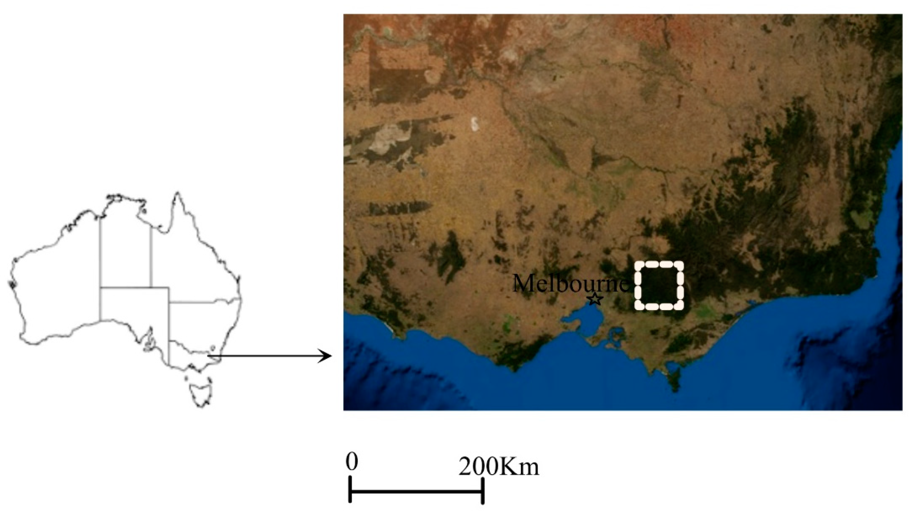
1.1. The Central Highlands of Victoria

A detailed map of the sampling points has been included in the Supplementary Data for this paper; this provides adequate detail to find approximate locations on “Google Earth”. This area encompasses the major catchments of the Goulburn River which flows north and the Thomson River which flows south, and small portions of the Yarra River catchment which flows east. These are important water sources for urban and irrigation water. The sampling area is within a polygon circumscribed by the towns of Warburton, Toolangi, Alexandra, and Woods Point; typically, this encloses a mixture of land tenures including State Forest, some private property, and large areas of reserves of various categories. A typical distance to drive from one side of the domain to the other would be about 70 km. Most of the study area is heavily forested and, other than the small town of Woods Point, there are few permanent residents within the forests. Around the edges of the forest (particularly to the north) are agriculture (including cropping and horticulture) and grazing areas. Streamflow from some areas to the north is used to produce hydro-electric power. The area has a history of gold mining and there is a small, historic and occasionally active underground gold mine at Woods Point. The areas are generally well-roaded, and most of the roads in the Goulburn River catchment are open to the public. In contrast, access to most areas of the Thomson Catchment is prohibited to the public on the grounds of water quality protection. There is no harvesting in most of the forested areas of the Yarra Catchments. Most catchments would usually have some disturbance due to roading associated with management, fire protection, and/or recreation. Fire protection in these areas demands a good road network irrespective of forest harvesting.

The study area has an annual rainfall in the 1000 mm to 2000 mm category, although “rain-shadow affects” can lead to considerable local variation. The combination of this and steep slopes leads to a network of well-aerated streams. The work of [3,4] in this environment has shown that many factors (including frequency of burning) are associated with active long-term landscape formation (erosion) in this environment. Studies on the Cropper Creek Paired Catchment Hydrology Project (e.g., [5]), approximately 100 km to the north-east but in a similar topography, showed that even completely “natural” streams are downcutting and that, if burnt, the rates of erosion can go up by two or three magnitudes for a few years. In particular, the Croppers Creek work showed active “backward head-cutting” in otherwise undisturbed catchments in these “foothill” environments. When burnt in 2006 [5], the catchments took about three years to return to their pre-burning hydrology.

1.2. Forest Harvesting in the Central Highlands

Forest harvesting has been a major economic land use in this general area for perhaps 120 years (see [6] for a forest history covering a part of the study area). Initially this was to provide materials to assist mining but more latterly the products have been sawlogs for structural and ornamental wood and pulpwood for paper making. The most favoured trees are of the “ash group” of Eucalypts (Eucalyptus regnans and E. delegatensis), but there are many “mixed species” trees (e.g., Eucalyptus obliqua, E. viminalis, and others) also used. The forests are classed as “native forest” and have a variable history. Some areas (particularly north of Toolangi) have a long and extensive history of forest management. Other areas have had less intensive silviculture over the years. The area was extensively (but not uniformly) burnt in the forest fires of 1939, and many forest areas have regenerated following these fires.

Figure 2 shows an example of a logging “coupe” taken from Google Earth and within the study area. Typically, this is a clear-felled or variable retention harvesting (retained unharvested islands) area of about 16–20 ha. A fundamental protection method is stream buffers in which harvesting activity is physically separated from flowing water. A good discussion of the effectiveness of these is found in [7,8,9]. Falling is predominately by machine falling. Logs are “snigged” (dragged) to a processing area (log landing), where sorting into grades and some processing (typically bark removal) are carried out. The logs are then trucked to a sawmill or paper manufacturing mill. Slopes can range up to 30° but with small areas >30° permitted to allow for local topographic variation in non-erodible soils. Layout (under the Victorian Government’s Code of Practice for Timber Production 2014) mandates a minimum of 20 m buffer strips along either side of streams (generally defined as watercourses with a defined stream bed). Various precautions are enforced to maintain water quality. These include the following:

• Lidar examination of areas and “recovery” of existing but overgrown logging roads to avoid earthworks where possible. Where possible, old roads are located, the vegetation removed, and the road formation reused.
• Protection of active streams with a riparian buffer of 20 m width from the stream edge. No trees are removed from these areas and roads and tracks do not penetrate the buffer zone. This gives an “infiltration zone” to absorb road and track runoff and protects the stream from insolation. Amongst others, refs. [7,8,9] give overviews of the efficacy of buffers in protecting water quality.
• Avoidance of large, exposed areas. In recent years, “variable retention harvesting” has been used. This ensures that more than 50% of a harvesting area is within one tree height of the retained forest, or that “islands” of trees are retrained within larger contiguous areas.
• Careful road layout to ensure roads are kept away from streams as far as possible; this reduces a major source of pollution [10].
• Avoidance of forestry work during prolonged wet weather.
• Avoidance of large accumulations of organic debris, usually by scattering this through the forest areas. This is for both fire and water quality protection, and to avoid off-site nutrient loss.
• Use of a “landing” for most works of storing and processing logs and other products. The site of the landing is marked to be well away from streams and water courses. The landing is well-drained with runoff passing into an “infiltration area”. At the cessation of logging, the landing is usually “rehabilitated” by ripping to remove compaction. Occasionally landings will be planted with local tree species to ensure regeneration but more commonly this is not needed.
• Strict supervision of works to ensure compliance with the many provisions of the Victorian Government’s “Code of Forest Practice”.

Methods of achieving forest regeneration vary from site to site. Often “seed trees” are left to ensure adequate seed of the dominant eucalypts. Some areas may be burnt to give an adequate seed bed (with seeding by aircraft or hand distribution), and very occasionally some areas may have a small amount of planting if the managers feel adequate regeneration is not being obtained. Methods of obtaining regeneration are usually assessed individually for the site; the methods selected generally conforms to the strictures of [11] or [12].

There is some variation in geology and edaphic factors over such a large area. The soils can be generically classed as “mountain loams”, which is a deep organic layer of vegetation and litter, passing into a mineral layer extensively occupied by tree roots, which then passes into a “saprolite” layer of decomposing rocks. Although the streams are incising themselves into the landscape, the soil is stable, and erosion by gullying or bank failure is not common. The soil is often many metres deep. After disturbance or fire, the vegetation regenerates quickly.

There have been many studies on the water quality aspects of forest harvesting. The most relevant to this paper is the paired catchment work of [13] examining impacts of logging in Melbourne’s water catchments. Many studies generally show that if the coupes are well laid out and the harvesting properly carried out, the water quality effects are transient and small. The effects can be partitioned into the impacts of harvesting (site disturbance giving enhanced turbidity lasting 1–2 years) and the impacts of roading. The latter is proportional to the traffic on the road [14,15]. Road maintenance for fire protection also can lead to enhanced turbidity if the road drainage passes into the stream network.

Most forest harvesting studies are “small-scale” and focus on the immediate vicinity of the harvesting, but one study that bears some similarity to this sampling project is [16]. This found that salvage logging after windstorms in Europe had no impact on water quality, including dissolved oxygen levels. The focus of most monitoring studies is determining the impact of harvesting on a specific reach of headwater (first or second order) streams rather than looking at the overall impact on a widespread group of higher-order streams. As the water moves downstream, it is particularly influenced by longitudinal dilution and dispersion [17] and cumulative effects of other variables. In contrast, this study sampled many streams, large and small.

1.3. Water Quality Standards

The streams of the Victorian Highlands flow into major dams used for both urban and rural water supplies. Water from the forest is known for its high quality in physical terms, usually for being clear. Ideally, the water quality is maintained as high as possible by good land-use practices. Water quality “ideals” defined for this area include:

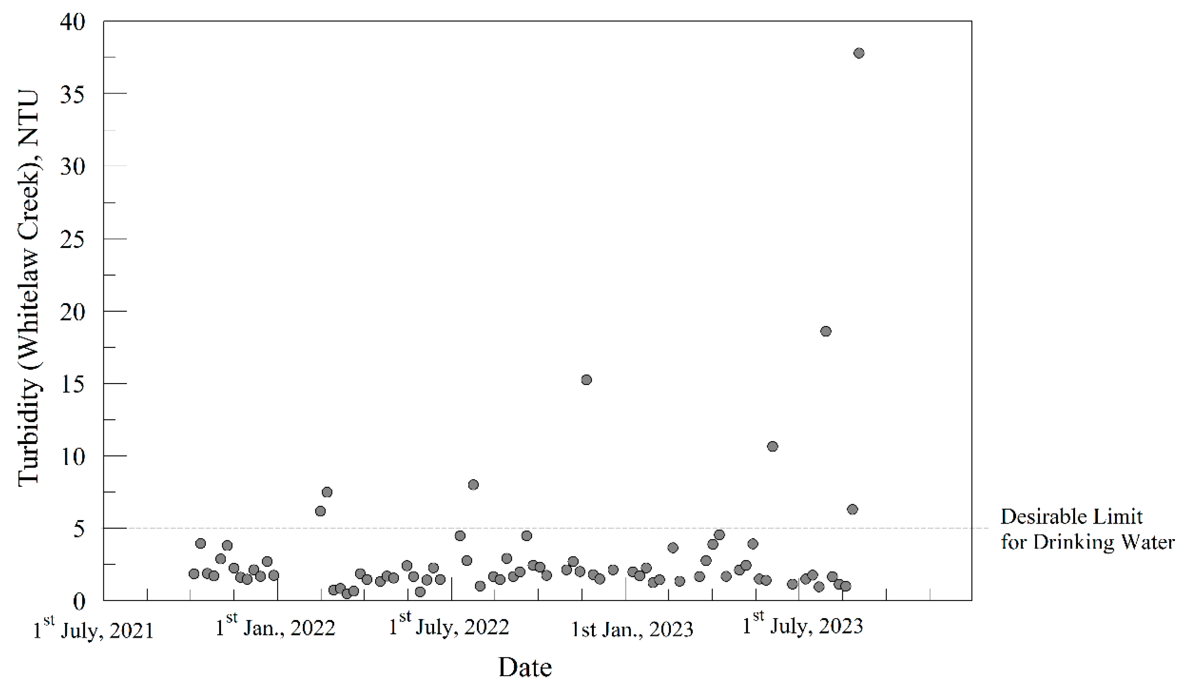
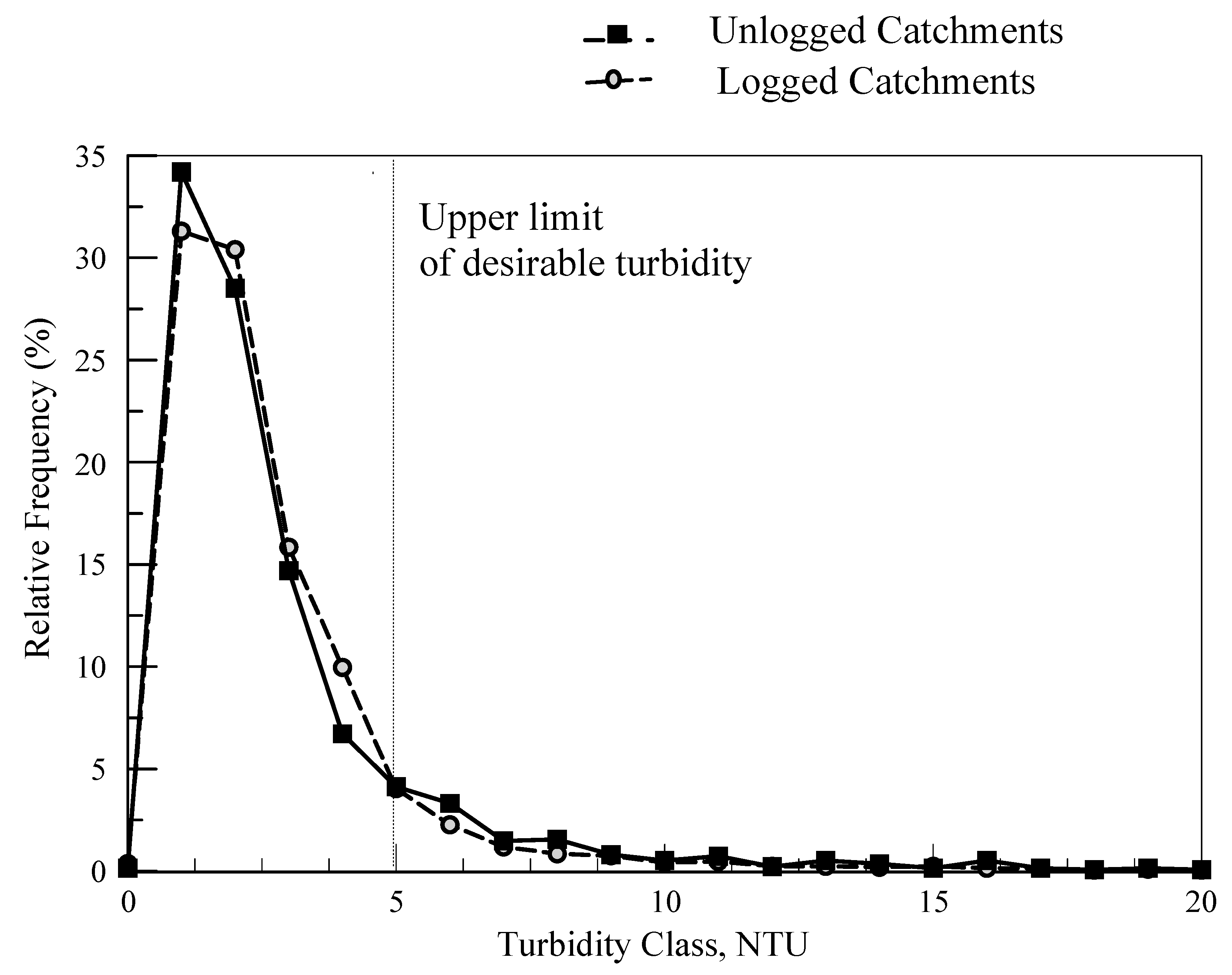
• Low values of water turbidity. Ideally, samples should have <5 NTU turbidity. In such streams, turbidity can be used as a general measure of sediment and soil contamination [18]. In general, there is a positive correlation between turbidity and parameters such as sediment load or water colour, but the actual regression differs from catchment to catchment. This is due to increased particulates being the usual cause of increased turbidity. It is known that much of the material causing increased turbidity is finely divided organic matter and hence increased turbidity may well be associated with decreased stream oxygen content [19].
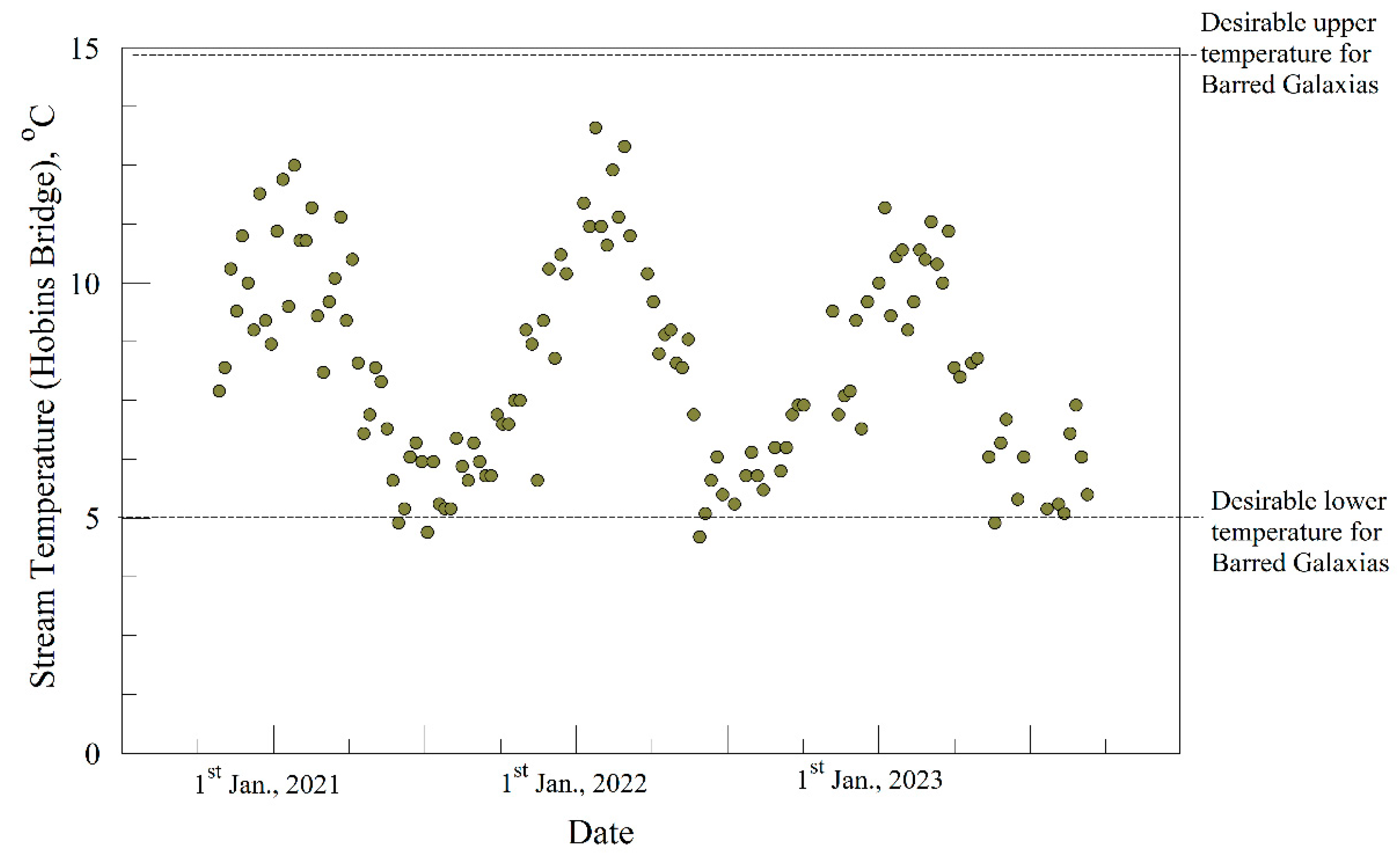
• Temperature of streams between 5 °C and 15 °C. These two ranges mark the “lowest” and “highest” temperature (defining an optimal range) of a small mountain fish (Galaxias fuscus—Barred Galaxias). These fish inhabit small, shallow, gravel-bottomed streams in mountainous areas. It has been hypothesised that, at higher temperatures, water may not carry enough oxygen to sustain fish life.
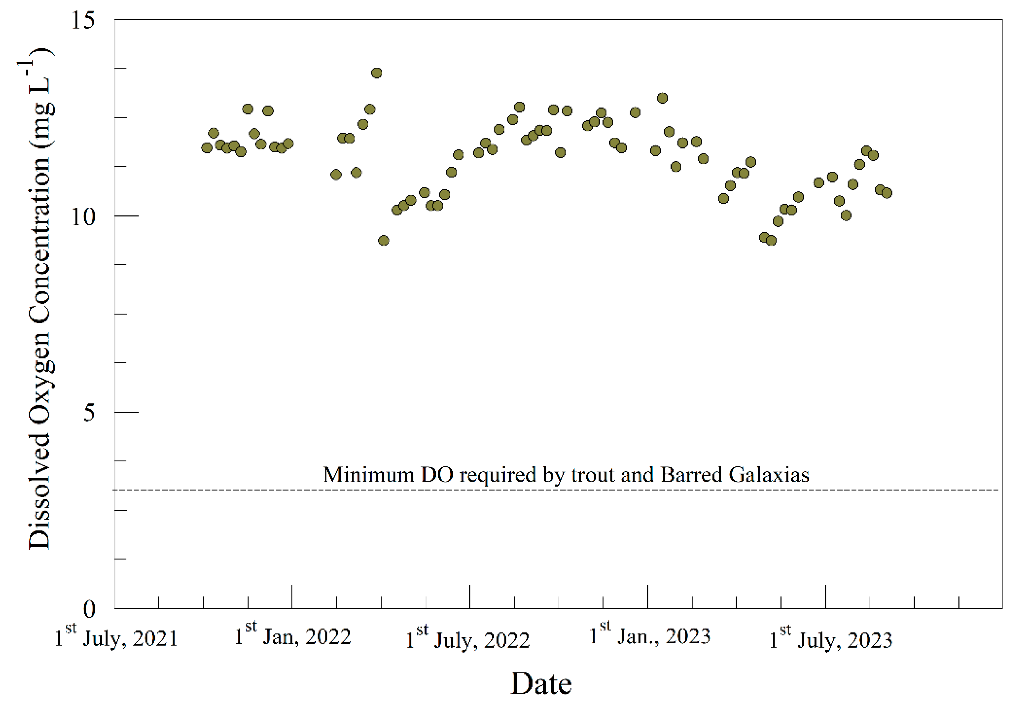
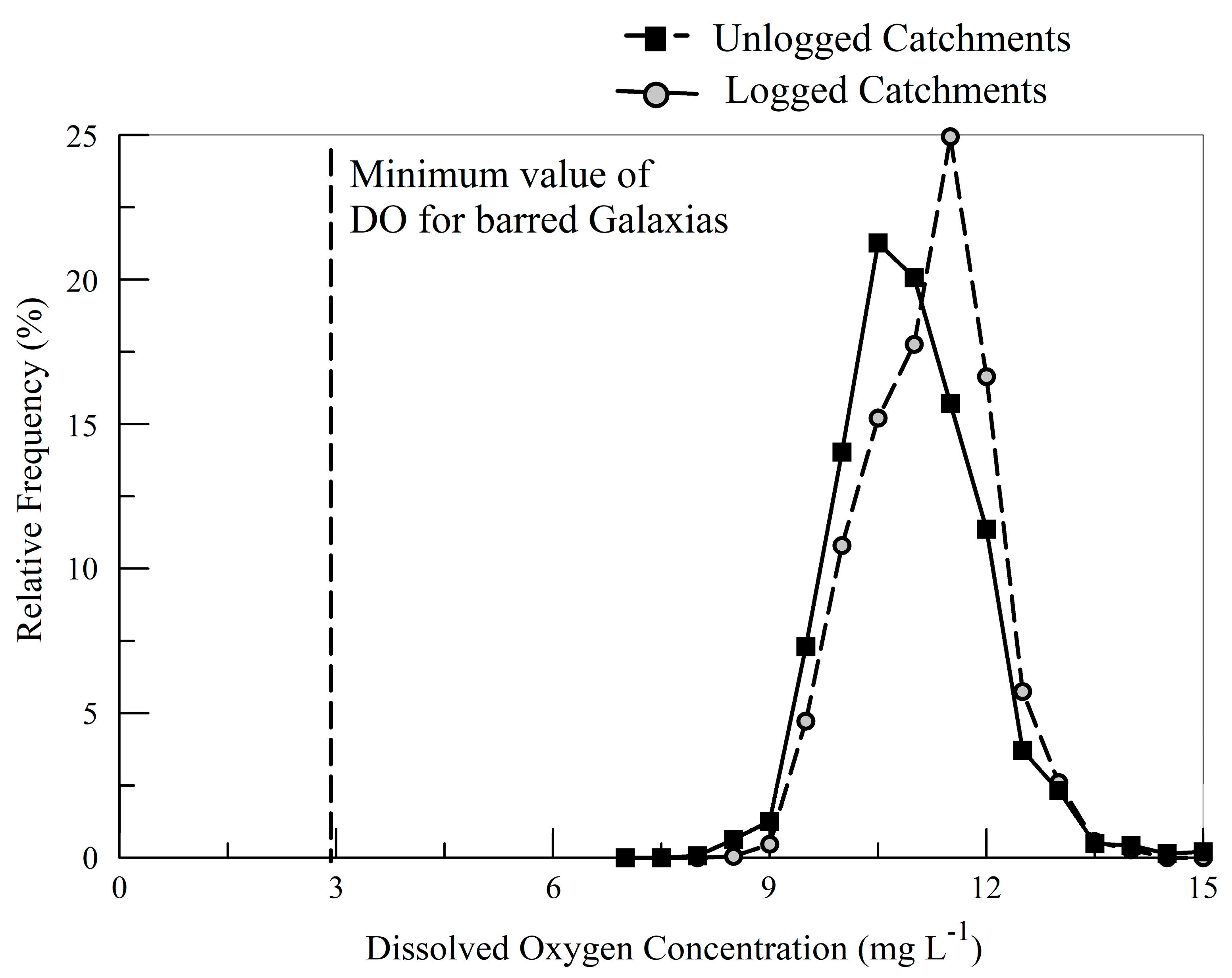
• Dissolved oxygen (DO) levels of >3 mg/L. This is viewed as the minimum DO for Barred Galaxias. In general, the streams from this mountain area flow over bedrock with a high gradient and many “white-water micro-rapids”, so the streams are highly oxygenated. The “white-water” represents entrainment of air in the flowing water. It has been shown that small headwater streams often have a diurnal variation in oxygen levels [20], and this can be an additional source of measurement error.

Regulations imposed by a number of government authorities can be used to restrict actions which may impair water, although it can be difficult to separate natural variation from land-use-induced variations. The high quality of the water can make measurement difficult because many water quality parameters are below the limit of detection for simple instruments. Most Australian enforcements are regulations rather than legislation, and these often suggest “guidelines” that should be met. If “tougher” enforcement is needed, there are a variety of mechanisms that can be used to give more stringent enforcement.

1.4. Advantages and Disadvantages of Water-Quality-Monitoring Networks

The role of this water-quality-monitoring network was to give a quantitative basis for examination of possible impacts of forest harvesting on the surface water quality of the regional stream and river network within a large, forested area. This has both a “real-time” and research component. If severe water quality effects were determined during on-going sampling, then there may be a cessation of forest harvesting together with appropriate amelioration works to reduce any impact. In the longer-term, the data give a record of variation from both natural and man-induced sources such as forest harvesting. Water-quality-monitoring networks fill an intermediate role in the world of hydrologic sciences. If catchment management effects are severe then the monitoring may show water quality impairment. More usually, the networks yield a “confused” signal composed of many inputs and cumulative effects of forest harvesting, roading, and natural entrenchment of streams. Refs. [21,22] thought that the establishment of objectives was the most important single step in implementing a monitoring network. Second was the need to develop a “testable hypothesis” to allow for an evaluation of the water data. There should be a sampling design that allows for a comparison (and/or differencing) of measurements.

Related to this is the question of what should be sampled. The Australian Drinking Water Guidelines [23] give a list of four water quality variables that should be sampled for headwater streams—turbidity, temperature, dissolved oxygen, and pH. Of these, turbidity, temperature, and dissolved oxygen were sampled in this monitoring network. The fourth parameter, pH, was found to be “difficult and unreliable” in pure headwater streams in the Croppers Creek Hydrology Project (e.g., [19]). This was due to the inconsistent readings from identical pH meters which calibrated perfectly in higher-ionic-strength standards. It was concluded that this was due to an absence of “buffering” in the low-ionic-strength stream water. Ideally, streamflow would be monitored too, but this requires a level of resources far beyond this case.

Ref. [18] points out that monitoring schemes such as this are efficient at characterising the state of water quality in rivers and streams but are not an efficient way of characterising the impacts of forest harvesting on water quality and quantity. This is because of the low intensity of sampling, the distance of the forest harvesting from the point of measurement, the small areas of forest harvesting involved, the small impacts of the forest harvesting, and the small number of parameters that can logically be measured. The recommendation was that if such detailed information on the hydrologic impact of logging is required, a “paired catchment” project is a better alternative. Ref. [18] also noted that concepts inherent in statistical analysis—“random sampling” and “normal distributions”—are usually, at best, approximated with water quality data. Amongst other things, this reflects difficulties of access to remote locations and the necessity for daytime samples. In this data analysis, we used a formal methodology based on “Student’s t-test” but also used visual examination of data distributions and distribution-free analyses based on rank correlation to examine the data.

2. Methods

2.1. Data Measurement

The basis of the monitoring was, ideally, a weekly visit to a network of water sampling points over almost three years (October 2020 to September 2023). At these visits, water temperature, turbidity, and dissolved oxygen levels were recorded following a rigorous organisational protocol. The sampling points were located on a variety of streams which had some logging upstream, forested catchments which had no logging, or “Community Reference Points” which were points located outside the forest and within local farming areas. The Community Reference points were on larger streams and rivers. It can be noted that, because the distances involved the remoteness of these sampling points, collection of the data was a major exercise involving many hundreds of kilometres of driving over remote forest roads for each day of sampling.

2.2. Parameters and the Data Set

Parameters were measured using Campbell Scientific YSI hand-held data loggers fitted with turbidity sensors, dissolved oxygen sensors, and temperature sensors. A full description of these can be found on the maker’s website [24]. A protocol of checking and calibration was developed to ensure consistency and long-term reliability (“VicForests Water Quality Sampling Guidelines”). The parameters measured were the following:

• Nephelometric turbidity (NTU units). This is a general measure of the suitability of water for drinking, with an NTU <5 indicating highly potable water. It is an optical measure given by the ratio of scattered-to-direct light transmission when a beam of light is passed into the water. Active streams are very dynamic in turbidity changes, with rain events giving transient higher turbidity early in the storm response hydrograph [18]. In general, the streams in this environment are “sediment-limited” and the turbidity response to rainfall quickly dissipates as available sediment moves downstream.
• Dissolved oxygen (“DO”) content (mg/L). In general, highly oxygenated streams support more in-stream biomass. Passage of stream water through large masses of decomposing vegetation can give a low oxygen content but such dumping of organic matter in streams is precluded by the terms of logging prescriptions and the “Code of Practice for Timber Production 2014” [25]. A priori, most streams in the data set from the “Logged” and the “Unlogged” groups would be expected to have a high oxygen content because of their high channel gradient and the resultant turbulence (which entrains oxygen). The minimum DO desirable for Barred Galaxias is 3 mg L⁻¹ [26].
• Stream temperature. Barred Galaxias ideally should have a stream water temperature between 5 °C and 15 °C. The removal of streamside vegetation by logging can possibly increase stream insolation, increasing the temperature. It has been shown that although the riparian buffer strips protect the streams from direct insolation, “sidelight” from outside the buffer strips can increase light intensity [7]. This possibly may lead to small, local increases in stream temperature.
• Catchment areas and areas of logging within the sampled catchments provided by VicForests staff using Victorian topographic mapping and their forest management records.

The sampling network used accessible points on a range of rivers and streams (both large and small). In rough country, reasonable access to the stream is a major criterion of selection. The stream sampling points can be characterised as:

• Streams or rivers with forested catchments and logging upstream of the sampling point (“Logged Catchments”). There were 19 such sampling points.
• Streams or rivers with forested catchments and no logging upstream of the sampling points (“Unlogged catchments”). Some of these areas do have small farm holdings embedded in the forest. There were 13 such sampling points.
• Streams or rivers referred to by community members as “needing to be protected”—“Community Reference Points”. Commonly these had areas of agriculture (grazing and cultivation) and farms upstream or in the vicinity of the sampling points. There were 9 such sampling points.

2.3. Examination of Frequency Distributions

Basic distribution parameters and the relative frequency distribution of the water quality parameters were obtained for the “logged” and “unlogged” data set to allow for a visual comparison of the relative frequency distributions. The author’s experience is that the human eye is a powerful discriminator of change, and that if no visual difference in distributions is apparent, it is unlikely that statistical tests will show differences.

2.4. Data Transformations and Hypothesis Testing

Preliminary examination of the data confirmed the common finding (e.g., [27]) of positive skewness in turbidity data. The turbidity data were transformed into the logarithmic value (base 10). This gave data with a statistical distribution approximating a normal distribution and allowed for the use of “Student’s t test” for the difference between means. This transformation is common in water quality studies (e.g., [24]). Our work followed the strictures of [28] who recommended the use of this transformation for physical measures of water quality but not for soluble constituents.

For such monitoring, the null hypothesis (H₀) is that there is no detectable effect of forest harvesting on our measures of water quality in the forested stream data. The alternative, H₁, is that there is a distinct harvesting effect visible in our water quality monitoring. In practical terms, H₀ implies that the set of data from the “logged catchments” is indistinguishable from that of the “unlogged catchments”. H₁ implies a significant difference between the means on the “logged” and “unlogged” streams. If the critics of forestry are correct, then this might be expected to be a “decrease in water quality”, manifested by increased turbidity levels, decreased oxygenation levels, and increased stream temperatures.

The initial catchment selection included a “control catchment”—Morning Star Creek (east of the small settlement of Woods Point, Victoria). This catchment had no logging and had a small, historic gold mine operating intermittently. The catchment is about intermediate in size and physical placement of all the catchments and had relatively few “missed readings”. The values of water quality measured in this were subtracted from those on all sites (“Logged”, “Unlogged” and “Reference”). This removed much seasonal variation (and autocorrelation) from the data and makes the data more compliant with the “normal distribution” expectation. The disadvantage of this is that the data are less interpretable in terms of our water quality experience. Formally, this is expressed as follows:

l_t = p_t − c_t

(1)

where p_t is the measure of water quality on a site at time t, c_t is the corresponding measure of the parameter on the Morning Star Creek at time t, and l_t is the residual value. The analysis of all water quality effects used the sequences of values of l_t. More formally, for the three parameters,

l_t = Log₁₀(p_t) − Log₁₀(c_t)

(2)

where p_t and c_t are measured turbidity values in the appropriate stream and the control stream (Morning Star Creek), and

l_t = p_t − c_t

(3)

where p_t is either the dissolved oxygen level or stream temperature on the appropriate stream and c_t is the corresponding measurement on the “control stream” (Morning Star Creek).

The data thus consisted of an l_t sequence for each of the three parameters for the 19 “logged” catchment streams and the 12 “unlogged” catchment streams (remembering that for 1 stream, “Morning Star” was used as a subtractor). The nine “Community Reference” streams or rivers were also similarly treated for comparison but not used in this phase of data analysis. For each catchment, the mean value of each sequence for each parameter case was computed. The l_t sequences were amalgamated for the “logged” and “unlogged” cases, and the mean and standard deviation values were computed. A “Student’s t test” to test the difference between the means was then used. If H₀ was to be rejected, then the “Student’s t” value was to be significant at a probability of <0.01. This methodology is common in water quality studies (e.g., [27]).

2.5. Spearman Correlation Examination of Parameters

Consider our set of 32 (i.e., 19 + 13) catchments with sampled water quality. Then, for each catchment, we have a mean value of turbidity, temperature, and dissolved oxygen. We also have a catchment area and an area of logging in each catchment. Suppose we rank the 32 catchments in order of mean turbidity, and rank them in order of logged area (with 0 for the unlogged ones): if there is a significant correlation between the rank orders (positive or negative), then we have reasonable grounds to infer a statistical relationship between these two variables. We developed correlation matrices for rank order using the Spearman correlation coefficients to ascertain whether there was information. This was, of course, supplemented by graphical examination of the data. The method avoids assumptions as to the underlying statistical distribution of the data set. An introduction to rank correlation coefficients is found in most statistical textbooks (e.g., [29]).

2.6. Comparison of Means with Reference Points

For each of the sampling points, mean values of the three parameters (using actual, not transformed values) were computed and displayed graphically. Inferences as to the water quality of the “forested catchments” (logged and unlogged) and the water quality of the “Community Reference Points” were drawn by visual comparison. This was to meet the concern of community members that logging would cause deterioration in water quality at their “Community Reference Points”.

Statistical examination used the facilities of the “ProStat Vs 6.5 for Window” (Poly Software International Inc., New York, NY, USA) statistical package and “Excel (MS Office 365)” spreadsheets. “ProStat” provides a comprehensive range of statistical facilities and deals with missing data well.

3. Results

3.1. Annual Distributions

Table 1. Details of the catchments in which water quality was sampled and their grouping.

Name (and Group)	Catchment	Logged	Land Use	Years Logged
	Area	Area
	Ha	Ha
Logged Group
Arnold Middle	2335	24.2	F, L	2017–2020
Arnold Lower	3101	23.7	F, L	2017–2021
Torbreck River	2933	17.6	F, L	2020–2022
Koala Upper	830	9.0	F, L	2021–2022
Koala Lower	1866	8.7	F, L	2020
Petty Metal Creek	455	10.5	F, L	2020–2022
Oaks Creek	6900	13.0	F, L	2017–2022
Springs Creek	4106	202.4	F, L	2017–2022
Matlock Creek	3868	162.7	F, L	2020–2021
Jordan Lower	4960	32.6	F, L	2021
Poole Gully	413	23.3	F, L	2021
BB Lower	1137	29.0	F, L	2020–2023
Whitelaw Creek	3976	4.1	F, L	2020
Eastern Outflow	12,720	5.4	F, L	2021
Dry Creek	3615	39.9	F, L	2019–2021
No. 6 Bridge	2342	37.1	F, L	2018–2021
Hobins Bridge	1851	12.6	F, L	2019–2021
Newmans Creek	273	6.0	F, L	2021–2022
No. 5 Bridge	968	51.9	F, L	2019–2023
Unlogged Group
Arnold Upper	339		F
Jordan Upper	3		F
Folkes Creek	7		F
Whitelaw Upper	1216		F
Upper Thomson River	1959		F
Middle Thomson River	11,992		F
No. 6 Tributary	163		F
Coles Creek	303		F
Sylvia Creek	662		F
Campbells Creek Upper	381		F
Campbells Creek Lower	815		F
Yea River Yea Link	489		F
Morning Star Creek	1123		F
Community Reference Group
(Agriculture)
Goulburn River, Walnut Res	374,896		P
Acheron River	50,498		P
Goulburn River, Woods Point	2527		F
Goulburn River, Alexandra	487,314		P
Yarra River, O’Shannessy			P
Steavenson River			P
Snobs Creek, Goulburn Vally Hwy	5055		P
Yea River, Smiths Road	2514		A
Yea River, Spraggs Bridge	3649		A

F, forest; L, logging; P, pasture; A, agriculture (cropping).

gives details of the actual sampling points, their geographic designation, the catchment area, and the area logged within the catchment. If all sites had been visited every week, then we would have had a data matrix of 41 sites × 151 visits × 3 parameters. For operational reasons, measurements in the “Matlock Block” did not start until almost a year after the others. Occasionally a site visit would be missed, or a parameter would not be measured at a site visit with a sampling rate of around 75% of the “sampling slots”. This gave a comprehensive data matrix. The rainfall variation in the years of measurement were viewed by observers as “to be expected”—neither unusually high (no high return period floods) nor low (no droughts).

Figure 3 shows a sequence of turbidity from Whitelaw Creek (in the “logged” set). The water is generally of high quality but occasionally a high turbidity value occurs. This was characteristic of all the turbidity data sets. Figure 4 shows a dissolved oxygen sequence from the same stream; it is highly aerated and well above the “lower limit” of the Barred Galaxias. This was typical of all the data sets from the upland streams. Figure 5 shows a sequence of stream temperature data from the stream at Hobins Bridge (in the “logged set” near the northern edge of the forest). A characteristic sinusoidal variation is shown with a minimum stream temperature of about 5 °C and a maximum stream temperature of about 13 °C. This was also typical of the data from the forested streams (see [18] for examples of this at both the annual and the daily level).

3.2. Frequency Analysis

Figure 6, Figure 7 and Figure 8 show the relative frequency distributions for untransformed values of turbidity, dissolved oxygen, and temperature.

Table 2. Characteristics of the frequency distributions of sampled data for the three parameters.

	Logged Catchments	Unlogged Catchments
Turbidity
Mean	2.4 NTU	3.0 NTU
Std Dev.	4.24	10.92
Skewness	12.96	18.86
Count	2108	1356
Dissolved Oxygen
Mean	11.0 mg L−1	10.8 mg L−1
Std Dev.	1.0	1.15
Skewness	2.82	2.24
Count	2170	1434
Temperature
Mean	9.4 °C	9.8 °C
Std Dev.	2.6	2.8
Skewness	0.37	0.29
Count	2187	1436

shows the means, standard deviations, and skewness of each of these distributions. In general, visually there appears to be little difference between the “Logged” and “Unlogged” set. All the sets show some positive skewness (which is characteristic of water quality data), but the turbidity data are particularly skewed. This is a common finding and led to the use of log-transformed data in hypothesis testing. In general, the data from both the “Logged” and “Unlogged” sets were well within the limits prescribed by drinking water standards or fish habitat requirements.

3.3. Hypothesis Testing

Table 3. Results of “Student’s t” tests on the means of transformed variables (19 means for the “Logged” set and 12 means for the “Unlogged” set).

	“Student’s t”	Probability	Ho
	Value
Turbidity	−0.032	0.977	Accept
Dissolved Oxygen	1.161	0.155	Accept
Temperature	−0.045	0.964	Accept

shows the results of the “Student’s t tests” for each of the water quality parameters using the sequence of mean values for the transformed values from each of the sampling points. These showed that the Ho is accepted (i.e., that there is no significant difference between the “Logged” and the “Unlogged” sets of data for the three water quality parameters). Figure 9, Figure 10 and Figure 11 show the means (of “transformed data”) together with the similarly transformed “Community Reference Points” data. Given the acceptance of the null hypothesis, in subsequent analyses, there should be no distinction between the groups. However, we have maintained this distinction in these illustrations. Some differences in the transformed sets of data from the “Forested” catchments and the “Reference” points are evident; these are discussed below using untransformed data.

3.4. Spearman Correlation Examination of Parameters

Table 4. Spearman rank correlation values for the 32 “forested” sampling points. The * represents significance at p = 0.05.

	Turbidity	DO	Temp.	Catchment Area
DO	−0.33
Temp	0.02	0.09
Catchment Area	0.33	0.19	0.1
Logged Area	0.01	0.33	0.08	0.53 *

shows a Spearman correlation matrix for the water quality parameters, catchment area, and logged area for the forested catchment data set. The statistical significance of the Spearman rank correlation coefficient is also indicated. Other than a weak correlation between the size of the catchment and the area of logging within it (significant at p = 0.05), we could find no significant correlation.

It is concluded that the parameters of turbidity, dissolved oxygen, and temperature are reasonably regarded as independent parameters in such a stream-monitoring network.

3.5. Comparison of Reference Sites with Forested Sites

Figure 12, Figure 13 and Figure 14 display the catchments. For reasons of community interest, the illustrations show the names of these. In particular:

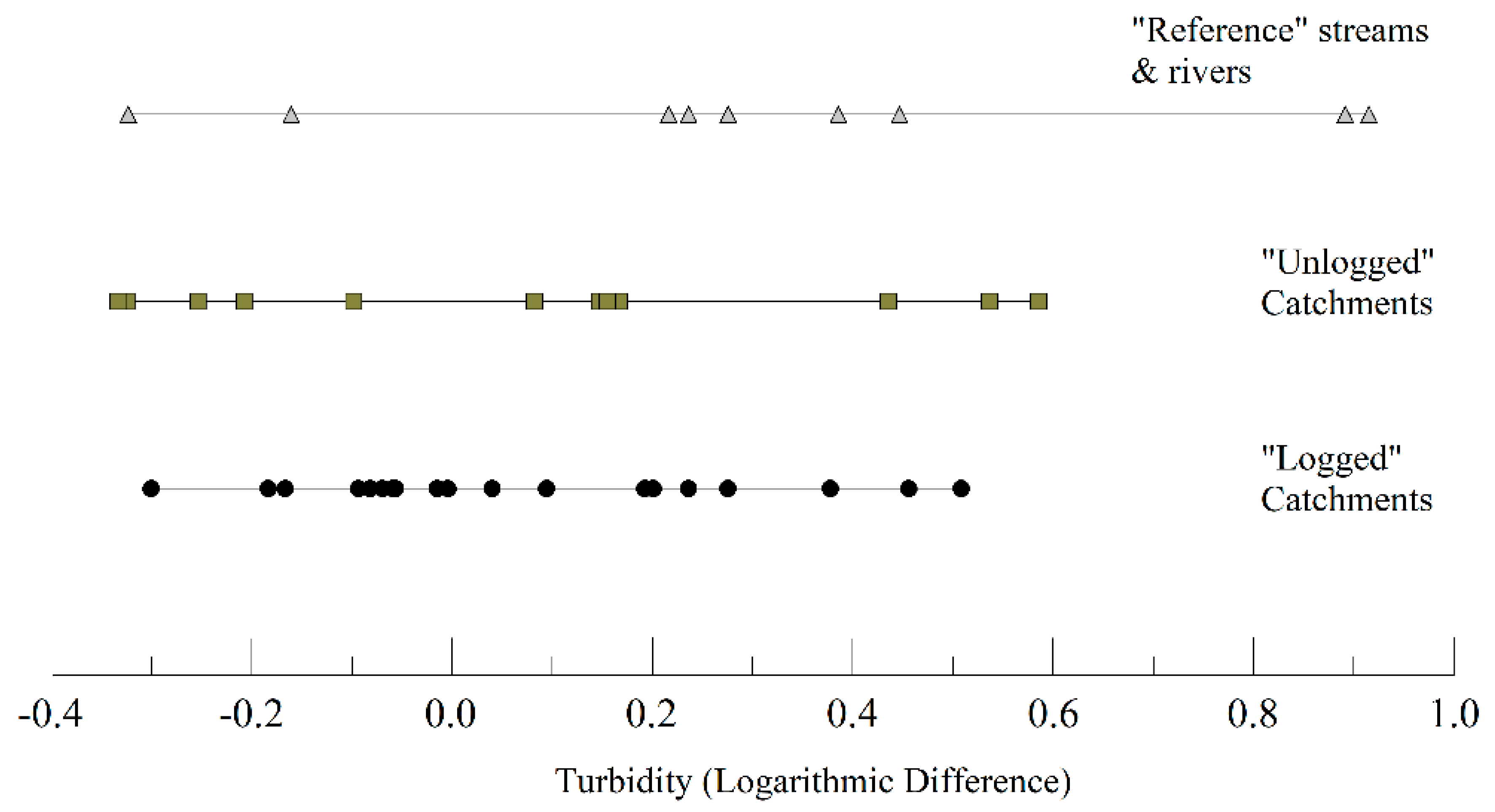
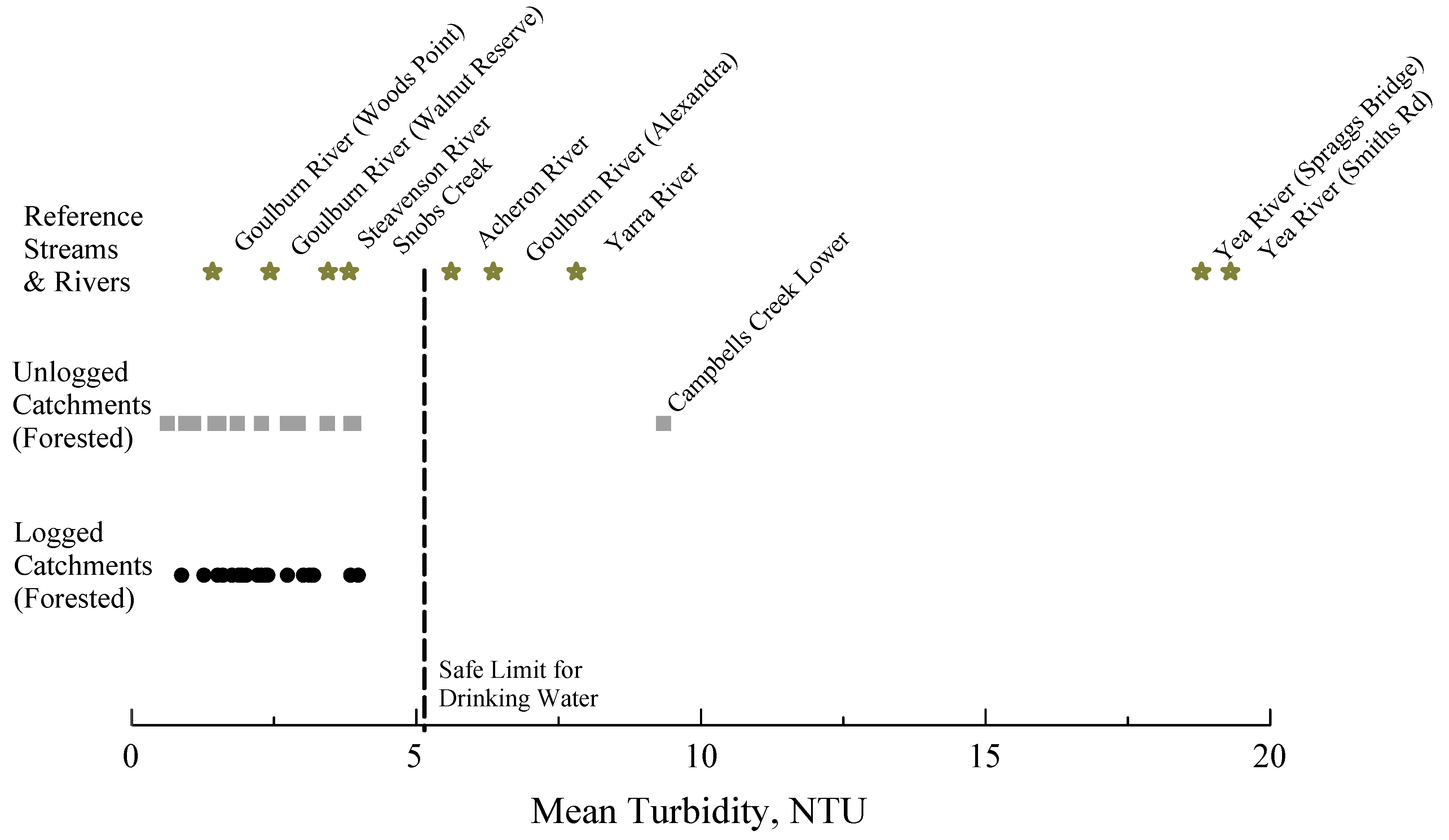
• Figure 12 (turbidity) shows the poor water quality associated with the Yea River (two sites) and, to a lesser extent, the Yarra River (outside of Melbourne’s catchment areas), the Goulburn River (at Alexandra), and the Acheron River. Each of these has substantial cultivation or other agricultural pursuits close to the water body. One can also find examples of small landslips associated with loss of riparian vegetation. The Campbells Creek data (unlogged forest) also show turbidity impairment; it is thought that this is associated with a small area of agricultural land within the forest.
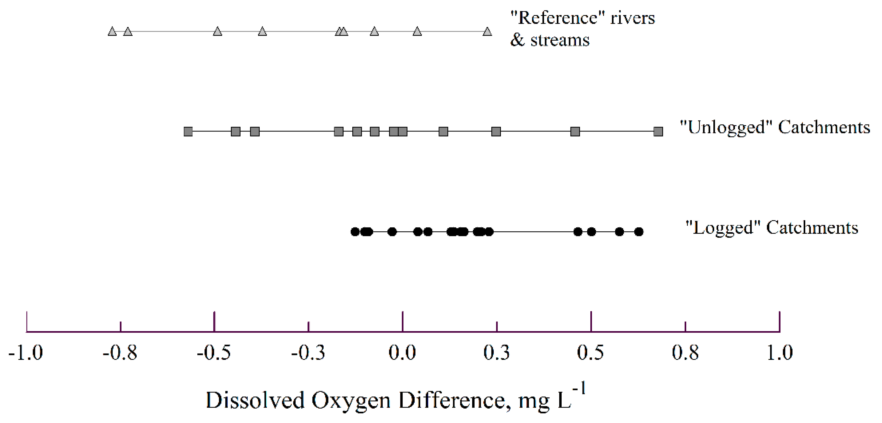
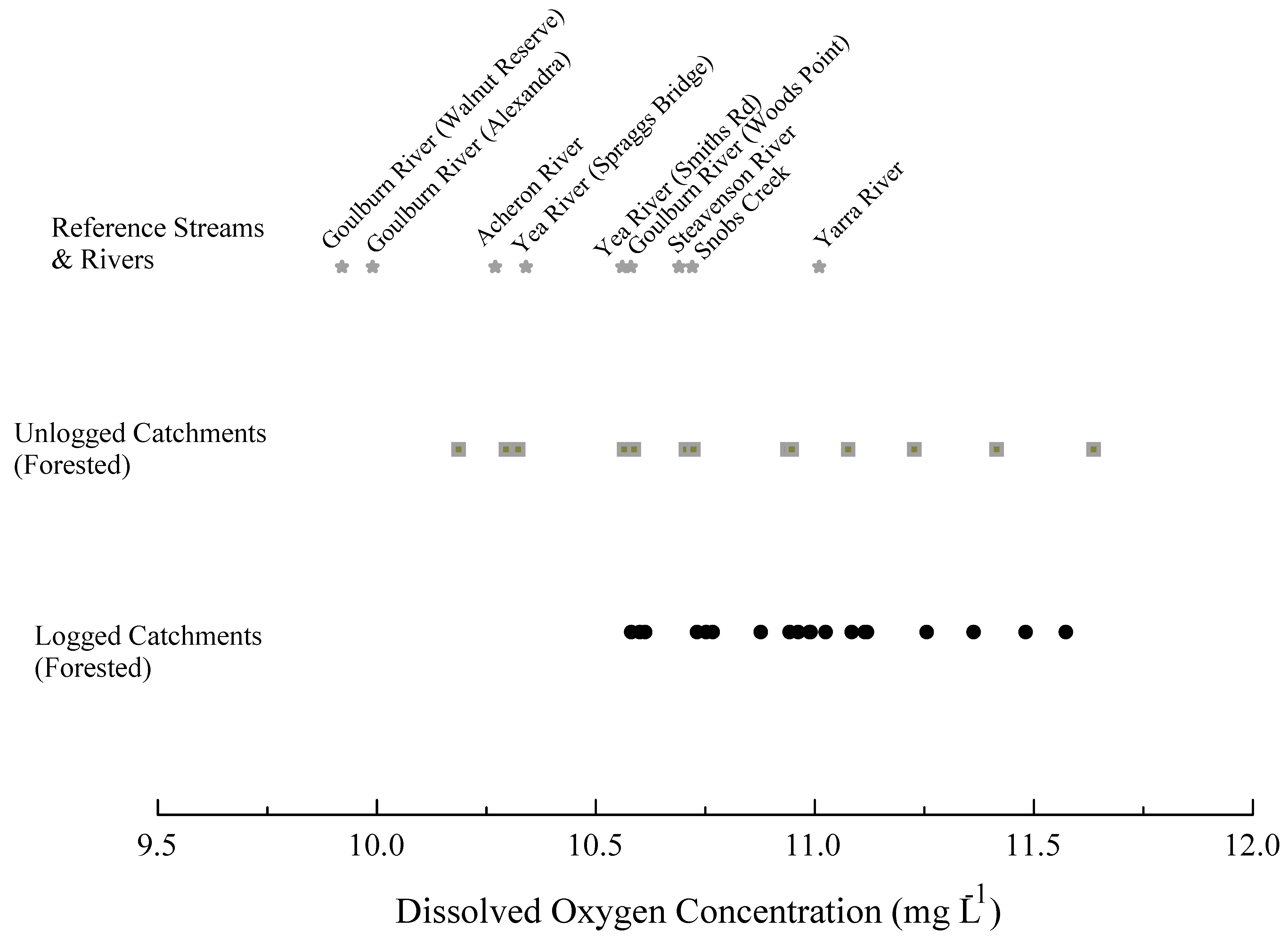
• The Goulburn River at “Walnut Reserve” and Alexandra shows lower levels of dissolved oxygen than the forested sites (Figure 13).
• In general, the forested catchments show lower stream temperatures than the “Reference Sites” (Figure 14). This is likely to be associated with the cooling effect of forest transpiration and the loss of riparian vegetation in the larger rivers.

4. Discussion

In summary, the results show no statistically significant difference between the water quality in the “Logged” and “Unlogged” set. We conclude that any forest harvesting “signal” entering the streams was too small to be detectable on the sampled streams. A reasonable conclusion is that the “logging water quality signal” is small and transient, is only locally apparent, and is obliterated in the “high noise” environments of the larger streams.

Analysis of the data produced many tables of data at various levels of aggregation. Graphical and correlation analysis were used to try to give “insights” into the data, but in general, not much was found. We sometimes found a weak negative correlation between temperatures and oxygen levels, but most such plots usually gave what appeared to be a “random scatter”. An example of such a weak negative correlation is given in Figure 15; this is shown for the Goulburn River data at Woods Point but not shown by the nearby, smaller Morning Star Creek. This reflects that river temperature is only one of many factors influencing the dissolved oxygen levels. There was a clearly sinusoidal relationship between water temperature and time of the year, but that is well known (e.g., [18]).

In general, the results show that the water quality in these upland streams emanating from forested catchments is generally good to excellent. They occasionally go on “water quality excursions” but these appear transient in nature. Fires in the catchments have extremely deleterious effects on all water quality parameters (e.g., [30]). For the period of sampling, there were no major forest fires in the area. The results also showed that the “Community Reference rivers and streams” which flowed through agricultural land commonly had higher turbidity values, stream temperatures, and generally lower dissolved oxygen content than the water quality from the upland streams emanating from forested catchments. This has been known for many decades in Victoria (e.g., [31]). Intensive cultivation near streams associated with crops such as strawberries appeared to be particularly detrimental to water quality.

The results of the analysis do highlight differences between “water quality monitoring” and more intensive but localised “paired catchment” sampling for research into logging. The results of this study give a picture of what is happening over a large area but have little to say about the actual impacts of logging in first-order streams bordering the logging. In general, the percentage of the catchment logged was about 2% with a maximum of 6% of the catchment area for Poole Gully. In paired catchment experiments, the “treatment” must usually exceed 20% of the catchment area to have a detectable effect [32]. Hence, it is unsurprising that such monitoring has not shown effects of forest harvesting on water quality in these streams.

It is also of interest to look at the mean values of Reference Sites with agricultural land use compared to our in-forest sites (Figure 12, Figure 13 and Figure 14). These indicate that once the streams leave the forest area, the turbidity and dissolved oxygen levels are, disappointingly, affected. Figure 16 shows an example of this.

5. Conclusions

A detailed monitoring project involving measuring three water quality parameters on a weekly basis at 32 sites over 2–3 years in regional streams and rivers was unable to find any detectable water quality influence of logging in the data sets. It was concluded that the water sampling showed no detectable adverse effects from “logging signals” in these stream networks. The water quality from the streams emanating from forested catchments ranged from good to excellent. In contrast, the water quality in “Reference Sites” outside the forest ranged from mediocre to good; this deterioration is likely to be associated with agricultural activities and cultivation. The sampling highlights the generally high quality of water in these small mountain streams relative to the streams leaving the forest environment and passing through agricultural land.

References

1. Indigenous Elder Stresses Importance of Snobs Creek—Friends of the Earth Melbourne (melbournefoe.org.au). Available online: https://www.melbournefoe.org.au/indigenous_elder_stresses_importance_of_snobs_creek (accessed on 30 June 2024).
2. Wilderness Society | Barred Galaxias (Vic). Available online: https://www.wilderness.org.au/news-events/barred-galaxias-vic (accessed on 30 June 2024).
3. Inbar, A. The Role of Fire in the Coevolution of Vegetation, Soil, and Landscapes in Southeastern Australia. Ph.D. Thesis, The University of Melbourne, Parkville, Australia, 2017. [Google Scholar]
4. Van der Sant, R.E.; Nyman, P.; Noske, P.J.; Langhams, C.; Lane, P.N.; Sheridan, G.J. Quantifying relations between surface runoff and aridity after wildfire. Earth Surf. Process. Landf. 2018, 43, 2033–2044. [Google Scholar] [CrossRef]
5. Bren, L.J. Hydrologic impacts of fire on the Croppers Creek paired catchment experiment. In Revisiting Experimental Catchment Studies in Forest Hydrology; Proceedings of a Workshop held during the XXV IUGG General Assembly in Melbourne, June–July 2011; IAHS Publication 353: Orlando, FL, USA, 2011; pp. 154–165. [Google Scholar]
6. Evans, P. Wooden Rails and Green Gold: A Century of Timber and Transport along the Yarra Track; Light Railway Research Society of Australia Inc.: Melbourne, Australia, 2022. [Google Scholar]
7. Dignan, P.; Bren, L.J. A Study of the Effects of Logging on the Understorey Light Environment in Riparian Buffer Strips in a South-East Australian Forest. For. Ecol. Manag. 2003, 180, 110–121. [Google Scholar] [CrossRef]
8. Bisson, P.A.; Claeson, S.M.; Wondzell, S.M.; Forster, A.D.; Steel, A.L. Evaluating Headwater Stream Buffers: Lessons Learned from Watershed Scale Experiments in Southwest Washington; General Technical Report, Pacific Northwest Resource Station, US Forest Service; U.S. Department of Agriculture Forest Service: Washington, DC, USA, 2013.
9. Sweeney, B.W.; Newbold, J.D. Streamside Forest Buffer Width Needed to Protect Stream Water Quality, Habitat, and Organisms: A Literature Review. J. Am. Water Resour. Assoc. 2014, 50, 560–584. [Google Scholar] [CrossRef]
10. Lane, P.N.; Sheridan, G.J. Impact of an Unsealed Forest Road Stream Crossing: Water Quality and Sediment Source. Hydrol. Process. 2002, 16, 2599–2612. [Google Scholar] [CrossRef]
11. Flint, A.; Fagg, P.C. Mountain Ash in Victoria’s State Forests. Silviculture Reference Manual No. 1; Department of Sustainability and Environment: Melbourne, Australia, 2007; 97p. [Google Scholar]
12. Sebire, I.; Fagg, P.C. High Elevation Mixed Species in Victoria’s State Forests; Department of Sustainability and Environment: Melbourne, Australia, 2009; 112p. [Google Scholar]
13. Grayson, R.B.; Haydon, S.R.; Jayasuriya, D.A.; Finlayson, B.L. Water Quality in Mountain Ash Forests—Separating the Impacts of Roads from Those of Logging Operations. J. Hydrol. 1993, 150, 459–480. [Google Scholar] [CrossRef]
14. Reid, L.M.; Dunne, T. Sediment Production from Forest Road Surfaces. Water Resour. Res. 1984, 20, 1753–1761. [Google Scholar] [CrossRef]
15. Sheridan, G.J.; Noske, P.J.; Whipp, R.K.; Wijesinghe, N. The Effect of Truck Traffic and Road Water Content on Sediment Delivery from Unpaved Forest Roads. Hydrol. Process. Int. J. 2006, 20, 1683–1699. [Google Scholar] [CrossRef]
16. Georgiev, K.B.; Beudert, B.; Bässler, C.; Feldhaar, H.; Heibl, C.; Karasch, P.; Müller, J.; Perlík, M.; Weiss, I.; Thorn, S. Forest Disturbance and Salvage Logging Have Neutral Long-Term Effects on Drinking Water Quality but Alter Biodiversity. For. Ecol. Manag. 2021, 495, 119354. [Google Scholar] [CrossRef]
17. Jobson, H.E. Prediction of Travel Time and Longitudinal Dispersion in Rivers and Streams; US Geological Survey: Reston, VA, USA, 1996; 69p.
18. Bren, L.J. Forest Hydrology and Catchment Management: An Australian Perspective, 2nd ed.; Springer: Berlin, Germany, 2023; 416p. [Google Scholar]
19. Hopmans, P.; Bren, L.J. Long-Term Changes in Water Quality and Solute Exports in Headwater Streams of Intensively Managed Radiata Pine and Natural Eucalypt Forest Catchments in South-eastern Australia. For. Ecol. Manag. 2007, 253, 244–261. [Google Scholar] [CrossRef]
20. Ulseth, A.J.; Hal, R.O.; Canadell, M.L.; Madinger, H.L.; Niayifar, A.; Battin, T.J. Distinct Air-Water Gas Exchange Regimes in Low and High Energy Streams. Natl. Geosci. 2019, 12, 259–263. [Google Scholar] [CrossRef]
21. MacDonald, L.H.; Smart, A.W.; Wissmar, R.C. Monitoring Guidelines to Evaluate the Effects of Forestry Activities on Streams in the Pacific Northwest and Alaska; University of Washington Water Centre: Seattle, WA, USA, 1991. [Google Scholar]
22. MacDonald, L.H.; Smart, A.W. Beyond the Guidelines: Practical Lessons for Monitoring. Environ. Monit. Assess. 1993, 26, 203–218. [Google Scholar] [CrossRef] [PubMed]
23. NHMRC. Australian Drinking Water Guidelines.6, Version 3.8, Updated September 2022; National Health and Medical Research Council: Canberra, Australia, 2011.
24. Water Quality: Products for Stand-Alone Water Quality Monitoring. (campbellsci.com.au). Available online: https://www.campbellsci.com.au/?gad_source=1&gclid=CjwKCAjw65-zBhBkEiwAjrqRMC0rJRMzgdyCIQS80eAFAu4gX_vOWJlU_P_weuQsVjK10rbhVuRlExoCzhMQAvD_BwE (accessed on 30 June 2024).
25. DEECA. Code of Practice for Timber Production 2014; Amended to 2022; Department of Energy, Environment, and Climate Action: Melbourne, Australia, 2022. [Google Scholar]
26. Raadik, T.A.; Fairbrother, P.S.; Smith, S.J. National Recovery Plan for the Barred Galaxias Galaxias fuscus; Department of Sustainability and Environment: Melbourne, VIC, Australia, 2010; 21p. [Google Scholar]
27. Helsel, D.R.; Hirsch, R.M. Statistical Methods in Water Resources. In Studies in Environmental Science; Elsevier: Amsterdam, The Netherlands, 2020; Volume 49. [Google Scholar]
28. Van Buren, M.A.; Watt, W.E.; Marsalek, J. Application of the Log-Normal and Normal Distributions to Stormwater Quality Parameters. Water Res. 1997, 31, 95–104. [Google Scholar] [CrossRef]
29. Steel, R.G.; Torrie, J.H. Principles and Procedures of Statistics: A Biometrical Approach, 2nd ed.; McGraw Hill Kogakusha: New Delhi, India, 1981; 633p. [Google Scholar]
30. Smith, H.G.; Sheridan, G.J.; Lane, P.N.; Nyman, P. Wildfire Effects on Water Quality in Forest Catchments; a Review with Implications for Water Supply. J. Hydrol. 2011, 396, 170–192. [Google Scholar] [CrossRef]
31. Mossop, D.C.; Kellar, K.; Jeppe, K.; Myers, J.; Rose, G.; Weatherman, K.; Pettigrove, V.; Leahy, P. Impacts of Intensive Agriculture and Plantation Forestry on Water Quality in the La Trobe Catchment; EPA Victoria Publication: Melbourne, VIC, Australia, 2013. [Google Scholar]
32. Hewlett, J.D.; Lull, H.W.; Reinhart, K.G. In Defense of Experimental Watersheds. Water Resour. Res. 1969, 5, 306–316. [Google Scholar] [CrossRef]
Figure 1. Map showing general location of the water monitoring. For detail, see the larger-scale map provided in the Supplementary Data.
Land 13 01217 g001
Figure 2. Extract of a satellite image showing forest harvesting sites north-east of Toolangi (Victoria). A three-year old variable retention harvesting (“Island retention”) coupe is shown, together with stream-protection buffers, roads, and unused haulage tracks. More mature forest can also be seen. Image courtesy of Google Earth.
Land 13 01217 g002
Figure 3. Plot showing measured turbidity in Whitelaw Creek during the monitoring period. Occasional turbidity “excursions” were found in all data sets.
Land 13 01217 g003
Figure 4. Plot of dissolved oxygen levels in Whitelaw Creek during the monitoring period.
Land 13 01217 g004
Figure 5. Plot of stream temperature at Hobins Bridge during the monitoring period. The same annual sinusoidal variation in stream temperature was evident on most records.
Land 13 01217 g005
Figure 6. Frequency polygon showing the relative frequency of turbidity classes for the “Logged” and “Unlogged” catchments.
Land 13 01217 g006
Figure 7. Frequency polygon showing the relative frequency of dissolved oxygen classes for the “Logged” and “Unlogged” catchments.
Land 13 01217 g007
Figure 8. Frequency polygon showing the relative frequency of temperature classes for the “Logged” and “Unlogged” catchments.
Land 13 01217 g008
Figure 9. Plot of the means of streams from the three groups for the difference in Log10 (turbidity). The zero corresponds to Morning Star Creek. The difference between overall means of the “Logged” and “Unlogged” groups is also shown. The two “Reference streams” on the far right are the Yea River (Smiths Road and Spraggs Bridge). This area has heavy cultivation.
Land 13 01217 g009
Figure 10. Plot of the means of streams from the three groups for the difference in dissolved oxygen levels. The two points with low dissolved oxygen levels in the “Reference group” are the Goulburn River at “Walnuts’’ Reserve and at Alexandra.
Land 13 01217 g010
Figure 11. Plot of the means of streams from the three groups for the difference in stream temperature. The zero is Morning Star Creek.
Land 13 01217 g011
Figure 12. Plot of the means of streams from the three groups for the mean stream turbidity (untransformed data).
Land 13 01217 g012
Figure 13. Plot of the means of streams from the three groups for the mean dissolved oxygen concentration (untransformed data).
Land 13 01217 g013
Figure 14. Plot of the means of streams from the three groups for the mean stream temperature (untransformed data).
Land 13 01217 g014
Figure 15. Dissolved oxygen level as a function of water temperature for the Goulburn River and the nearby, smaller Morning Star Creek at Woods Point, Victoria.
Land 13 01217 g015
Figure 16. Turbid runoff from cultivation passing into a stream near Toolangi (Victoria) compared with runoff from a recently harvested site on the same day.
Land 13 01217 g016