Achieving Sustainable Land Use Allocation in High-Altitude Area by 2030: Insights from Circle Structure and Scenario Predictions for Production–Living–Ecological Land in Xining Marginal Area, China

Abstract

The paper focused on the Xining marginal area, providing the concept of land use competitive advantage, employing the PLUS and PFCI model to simulate production–living–ecological (PLE) land in 2030, and revealing the relationship between regional land interactions and sustainable land allocation. The results indicate that the following: (1) By 2030, the land use of the Xining marginal area is primarily production and ecological land, with approximately 0.1% of living land; however, living and production land will increase while ecological land will decrease in general, and the growth momentum of urban and other living space in government-seated regions is stronger. (2) The PLE land does not exhibit a piecemeal expansion pattern, as it is influenced by mountains and rivers. Agricultural production land and grassland ecological land have advantages for development, whereas urban living land has just development potential. (3) Developing the corresponding lands in the dominant regions can result in sustainable land allocation, and five nexus approaches are proposed for the sustainable allocation of PLE land in the Xining marginal region. The study addresses the interaction of different land use types across regions rather than examining them separately, and we provide significant insight into whether the Qinghai Tibet Plateau should be urbanized.

1. Introduction

Sustainable development has become a common concern in metropolitan and remote areas due to the continual growth of urbanization and the stronger use of space resources [1]. It has become an important global issue as all nations strive to coordinate their economies, societies, and environments [2]. The sustainable development goals (SDGs) were released by the UN in 2015 with the purpose of helping nations develop sustainable development plans [3]. In fact, land use plays a crucial role in achieving the SDGs, as the two are in good agreement and the evolution of land use has a deep impact on the realization of SDGs [4]. As a carbon source or sink, land use serves as one of the leading factors responsible for global climate change (SDG 13). Besides, it also acts as a pollution source and sink, and thereby has a great impact on ecological protection (SDG 14–15). Land is the main carrier of food and plays a role that cannot be underestimated in ensuring food security (SDG 2) [5].

The Qinghai–Tibet Plateau is one of the largest carbon sequestration regions in China and an important control area for global atmospheric circulation and water cycle. The protection and allocation of its land resources will contribute to the mitigation of global climate issues and the achievement of SDGs [6]. Xining, as the locomotive driving the development of the Qinghai–Tibet Plateau, has witnessed a gradual acceleration in its urbanization process, leading to an increased demand for the utilization of spatial resources. In response, research proposes the concept of urban marginal areas, which refers to the transition area between the city and the countryside as well as the sub-center or new urban area [7], and it is also the area most affected by urban elements as the main space for population and land use growth [8]. Marginal area faces multiple challenges such as the daunting task of coordinating land use with construction and ecological protection, where different spatial structures and multiple land use types intertwine in a subtle manner, with a mixture of rural, suburban, industrial parks. wholesale markets and undeveloped interstitial spaces, presenting a situation of uncontrolled living space, disorderly production space, and imbalanced ecological space. Therefore, the Chinese government has proposed production–living–ecological (PLE) land as the basic framework for land use planning and management to achieve sustainable social, economic, and ecological development [9]. The conflicts between PLE land essentially manifest as competition and conflict between spatial resources for different purposes and functions within the same area, resulting from the interaction of human–environment relationships. Inconsistency between PLE land exacerbates the contradictions between economic development, ecological protection, and cultivated land conservation, seriously threatening the sustainable use of land. Will the Xining marginal area embark on the way of rapid urbanization? How to optimize the allocation of land use patterns to achieve social, economic, and ecological balance and stability? These have become key issues to be solved urgently for sustainable development in the Xining marginal area.

Scholars have conducted in-depth studies on the impacts of land use change or allocation on sustainable development, with the efforts mainly on risk identification and spatial optimization. From the perspective of risk identification, some scholars have engaged in ecological risk analysis based on future land use projections [10], and the assessment of land use policies on sustainable development [11]. From the perspective of spatial optimization, land use optimization is based on the theory of comparative advantage, which adjusts and optimizes the proportion of land types under certain constraints to improve the overall benefits of land use [12]. Scholars have studied the optimal allocation of land use at different scales such as global [13], continental [14], national [15], regional [16], watershed [17], and farm [18], as well as single ecosystems such as agriculture [19] and urban [20]. Mathematical models are the frontiers of land use optimization, which can be divided into two categories: quantity structure optimization models and spatial distribution optimization models. Firstly, due to the complex non-linear relationship between PLE land and driving factors, it is hard to construct an optimization model with traditional quantity structure methods. Secondly, spatial distribution optimization models mainly solve the spatial configuration problem of land use to achieve optimal suitability, such as the CLUE-S model [21], Cellular automata (CA) [22], multi-agent systems (MAS) [23], and PLUS (patch-generating land use simulation) model [24]. With an adaptive inertia mechanism and a roulette wheel selection mechanism, the PLUS model improves simulation accuracy based on the FLUS model [25]. In addition, it also offers the development probability of each category with the Random Forest Algorithm, making up for the deficiency of the CA-Markov model in exploring the change law of land use, and overcoming the difficulty in dynamically modeling the patch-level changes in natural land types in time and land. However, all the land types interact with each other and affect all the SDGs, but each is often studied in isolation. On the one hand, developing a land or achieving a sub-goal may result in the impossibility to balance other lands or achieve other sub-goals [26]. On the other hand, different entities or regions have different development objectives and different spatial trends, and stakeholders may contradict each other in achieving policy objectives in different regions [27,28]. Therefore, it is imperative to take the interests and endowments of different regions into account for integrated allocation, and to consider interactions among more sectors, across scales, and between adjacent and distant places, and linkages with SDGs [26].

In this article, we emphasize nexus approaches [29] to understand the connections and synergies on spatial distribution optimization, and propose the concept of land use competitive advantages, i.e., the dominance of a region in developing a certain land use type. Correspondingly, we propose Pythagorean fuzzy conflict information (PFCI), a combination of the Pythagorean theorem and fuzzy theory, to calculate competitive advantages. As the mismatch between one-size-fits-all policies and complicated regional relationships violates the principle of nexus land use allocation, this article aims to address the above problem from the perspective of interactions between different land types and different regions, rather than considering them in isolation. Given the particularity of the Xining marginal area and sustainable development goals, we set up four scenarios, namely, natural development, urban development (SDG8, economic development), cultivated land conservation (SDG2, Zero Hunger), and ecological protection (SDG13, Climate action) to simulate the 2030 spatial pattern of PLE land in the Xining marginal area by the PLUS model. Then, we further propose the concept of land use competitive advantages and improve PFCI by introducing concepts such as the maximum doughty coalition, the trisections of four types of sets, and viable strategies. Based on this, we identify sets of advantageous land use types and regions. Ultimately, we put forward policy references to achieve nexus approaches to land use sustainable allocation based on regional endowments. In summary, our research aims to answer the following questions:

(1) Will the Xining marginal area embark on the path of rapid urbanization?

(2) How do the advantages of certain land use types and regional endowments reveal the sustainable allocation of land use?

(3) What nexus approaches should we take to achieve sustainable land use allocation in the Xining marginal area?

2. Materials and Methods

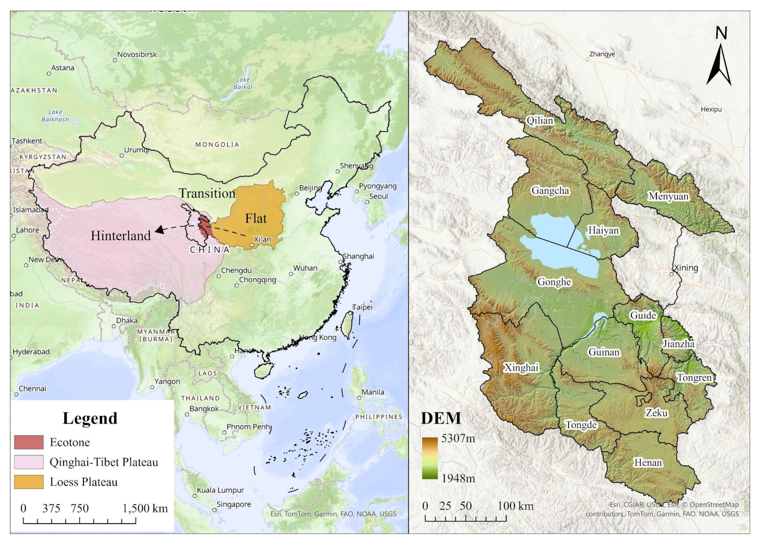
2.1. Study Area

The Xining marginal area is located in Qinghai Province, including three administrative regions: Haibei Tibetan Autonomous Prefecture (Menyuan Hui Autonomous County, Qilian County, Haiyan County, and Gangcha County), Hainan Tibetan Autonomous Prefecture (Gonghe County, Tongde County, Guide County, Xinghai County, and Guinan County), and Huangnan Tibetan Autonomous Prefecture (Tongren City, Jianzha County, Zeku County, and Henan Mongol Autonomous County). Among them, Haiyan County, Gonghe County, and Tongren City are government-seated regions (Figure 1).

2.2. Data Sources

The data in this paper consist of a land dataset, a socio-economic dataset, and a natural dataset.

The input datasets for the PLUS model are the 30 m land use for the years 2015 and 2020, and they have been reclassified as production–living–ecological (PLE) land, which is based on their dominant and secondary functions [30,31,32,33]. Ecological land refers to the land that maintains human survival, including climate regulation, water regulation, the mitigation of emergencies, and soil conservation. Therefore, its evolution is an effective way to reveal the implementation of SDG 13 (Climate action). Production land refers to the land where products and services can be directly obtained as labor objects or produced. It functions as a carrier for social production, including food supply, raw material production, energy, and mineral production [31]. Therefore, its evolution is an effective way to reveal the implementation of SDG 2 (Zero Hunger). Living land is primarily aimed at human production, leisure, and living. While providing resources and giving impetus to economic growth, it also creates a comfortable living and entertainment environment [21]. Therefore, its evolution is an effective way to reveal the implementation of SDG 8 (economic growth). It should be noted that there are no paddy fields and beaches in the study area (

Table 1. Classification of lands and their sub-lands.

Land	Sub-Land	Corresponding Land Use Type
Living land	Urban living land	Urban built-up land
	Rural living land	Rural residential land
	Other living land	Other built-up land
Production land	Agricultural production land	Dry land; Canal
Ecological land	Forest ecological land	Forest; shrub land; wood land; other forest
	Grassland ecological land	High grassland; mid grassland; low grassland
	Water ecological land	Lake; reservoir-pond; snow; shallow
	Other living land	Sand; gobi; saline; swamp; barren land Rock; others

).

The process of land cover change in the Xining marginal area has a fundamentally different driving mechanism compared to inland regions. Firstly, there is an active adaptation of human activities and urban construction to the fragile ecological environment of the high-altitude, cold, and oxygen-deficient plateau. In this active adaptation process, elevation serves as the primary constraint on the expansion of human activities, with most of the development of the plateau towns and agricultural activities limited to the river valleys. As an important evaluation criterion for urban development and cultivated land conservation, the slope profoundly affects the evolution of built-up land and cultivated land. Therefore, among the natural driving factors, we have selected these two indicators. Secondly, there are progressive processes, as well as external driving processes. The progressive process mainly considers the inertia of development based on the existing towns, as the scale of towns in the Xining marginal area is generally small. New construction land is primarily concentrated around the existing towns where the population density and industrial activities are relatively vibrant. Moreover, the driving force for urbanization in the Qinghai–Tibet Plateau is mainly top-down government-led initiatives. Thus, we have chosen population density, GDP, and government locations as the indicators for such processes. The external driving process primarily includes the impact of tourism and targeted assistance, both of which depend on the transportation infrastructure conditions. Additionally, when operating the PLUS model, it is essential to consider the volume of data. After multiple attempts and assessments of the factors’ driving force, we ultimately selected “distance to primary roads” as the indicator for transportation as an external driving force (

Table 2. Data sources.

Data	Sub-Data	Year(s)	Resolution	Sources
Land use dataset	PLE land classification in Table 1	2015, 2020	30 m	https://www.resdc.cn/ accessed on 4 August 2022
Socio-economic dataset	Population	2020	1 km	https://www.resdc.cn/ accessed on 4 August 2022
	GDP	2020	1 km	https://www.resdc.cn/ accessed on 4 August 2022
	Primary roads	2020	Vector data	Open Street Map
	Seat of county government	2015	Vector data	http://www.dsac.cn/ accessed on 4 August 2022
Natural dataset	Elevation	2015	1 km	https://www.resdc.cn/ accessed on 4 August 2022
	Slope	2015	1 km	https://www.resdc.cn/ accessed on 4 August 2022

).

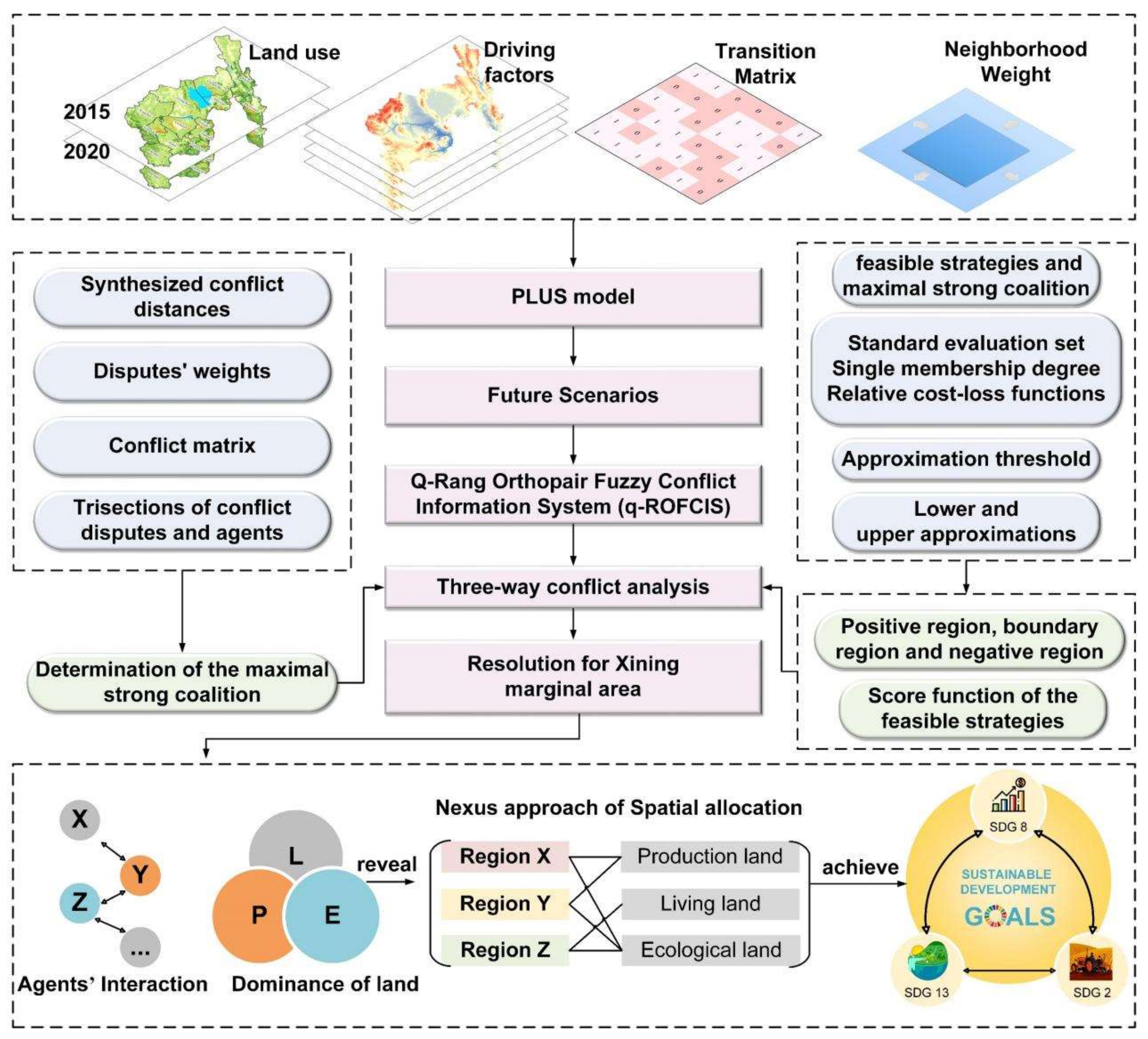
2.3. Patch-Generating Land Use Simulation (PLUS) Model

The PLUS (patch-generating land use simulation) model was proposed by Liang et al. [24] for simulating land use change. We set up a natural growth scenario (scenario A) and urban development scenario (scenario B) in this paper for simulating the land use pattern of the Xining marginal area according to the existing trend and rapid urban development. In addition, based on the previous studies [34], we set up the sustainable development goals and policies currently implemented in China for the “red line of ecological protection, the red line of cultivated land, and the urban development boundary”, the cultivated land conservation scenario (scenario C), and the ecological protection scenario (scenario D), and the transition matrix of each scenario is shown in

Table 3. Transition matrix in PLUS.

	Scenario A						Scenario B						Scenario C						Scenario D
	a	b	c	d	e	f	a	b	c	d	e	f	a	b	c	d	e	f	a	b	c	d	e	f
a	1	0	1	0	1	1	1	0	0	0	1	1	1	0	0	0	0	0	1	1	1	1	1	1
b	0	1	1	0	0	1	1	1	0	0	1	1	1	1	1	0	0	1	0	1	0	0	0	0
c	1	1	1	1	1	1	1	0	1	0	1	0	1	1	1	1	1	1	0	1	1	1	0	0
d	1	0	1	1	0	1	0	1	1	1	1	0	1	0	1	1	0	1	0	0	0	1	0	0
e	0	0	0	0	1	0	0	0	0	0	1	0	0	0	0	0	1	0	0	0	0	0	1	0
f	1	1	1	1	1	1	1	1	1	1	1	1	1	1	1	1	1	1	1	1	1	1	1	1

Notes: (1) According to the classification system of land use monitoring using remote sensing of the Chinese Academy of Sciences, we combined the land use types into cultivated land, forest, grass, water, built-up land, and bare land in the transition matrix. In the table, a represents cultivated land (including dry land), b represents forest (including forest, shrub land, wood land, and other forest), c represents grass (including high grassland, mid grassland, and low grassland), d represents water (including canal, lake, reservoir-pond, snow, and shallow), e represents built-up land (including urban built-up land, rural built-up land, and other built-up land), and f represents bare land (including sand, gobi, saline, swamp, barren land, rock, and others). (2) The 0 means conversion to another land type is prohibited, and 1 means conversion to another land type is allowed.

.

The neighborhood weight parameter indicates the strength of the expansion capacity of the land type. According to Wang et al. [35], the change in TA (Total Area) of each land type at the same time scale can better reflect its expansion intensity. The dimensionless value of TA change conforms to the parameter requirements of the model neighborhood weight in terms of data meaning and data structure. Therefore, the calculation of the PLUS model neighborhood weight in this study is as follows:

$$W={\displaystyle \frac{\Delta {TA}_i-\Delta {TA}_{min}}{\Delta {TA}_{max}-\Delta {TA}_{min}}}$$

where ΔTA_i represents the amount of TA change in the land type; ΔTA_min represents the land type with the smallest amount of change; ΔTA_max represents the land type with the largest amount of change. Based on the TA changes in all the land use types in the Xining marginal area from 2015 to 2020, we calculated the neighborhood weight of each type as shown in

Table 4. Weight of each land use type according to ΔTA.

Variety	Dry Land	Forest	Shrub Land	Wood Land	Other Forest	High Grassland
ΔTA	−193.77	35.46	−1743.39	−150.84	9.27	22,166.10
Weight	0.61	0.62	0.59	0.62	0.62	1
Variety	Mid grassland	Low grassland	Canal	Lake	Reservoir-pond	Snow
ΔTA	−9190.26	−35,812.26	−1224	11,317.32	6207.93	1429.20
Weight	0.46	0	0.60	0.81	0.72	0.64
Variety	Shallow	Urban built-up land	Rural residential land	Other built-up land	Sand	Gobi
ΔTA	−74.34	827.55	519.75	15,283.26	−8804.97	18.09
Weight	0.62	0.63	0.63	0.88	0.47	0.62
Variety	Saline	Swamp	Barren land	Rock	Others
ΔTA	101.97	−1710.72	51.30	943.38	−6.03
Weight	0.62	0.59	0.62	0.63	0.62

.

2.4. Construction of Pythagorean Fuzzy Conflict Information (PFCI) Model

Pythagorean fuzzy conflict information (PFCI) is an effective tool for modeling real-world decision-making problems involving information uncertainty. It originated from the fuzzy sets (FSs) proposed by Zadeh [36]; Yager [37] proposed PFSs in 2014. Afterwards, he introduced q-ROFSs to retain more imprecise information [37]. Looser restrictions allow for more flexible application of q-ROFSs, which can be used to solve land use conflicts. By this, the calculation of competitive advantages is possible by defining the conflict distance and conflict function to describe the uncertainty in the conflict, and then calculating and ranking the scoring function based on the feasible strategies and rough set theory. It is possible to find the internal causes of the conflict and find a feasible solution. The calculation process is as follows:

Definition: A q-ROFS B in terms of a finite universal set X is defined as follows:

$$\mathcal{B}=\left\{〈x,{\mu }_b\left(x\right),{\upsilon }_b\left(x\right)〉\right|x\in X\}$$

(1)

where ${\mu }_b\left(x\right)$ and ${\upsilon }_b\left(x\right)$ represent the degree of the membership and non-membership of element $x$ with respect to the set $\mathcal{B}$; simultaneously, ${\mu }_b\left(x\right)$ and ${\upsilon }_b\left(x\right)$ satisfy the restriction $q\ge 1$, $0\le {\left({\mu }_b\left(x\right)\right)}^q\le 1$, $0\le {\left({\upsilon }_b\right(x\left)\right)}^q\le 1$ and $0\le {\left({\mu }_b\left(x\right)\right)}^q+{\left({\upsilon }_b\right(x\left)\right)}^q\le 1$, and $〈{\mu }_b\left(x\right),{\upsilon }_b\left(x\right)〉$ is a q-ROF number (q-ROFN) denoted by $\rho =〈{\mu }_b,{\upsilon }_b〉$. In addition, $r_b\left(x\right)=\sqrt[q]{{\left({\mu }_b\left(x\right)\right)}^q+{\left({\upsilon }_b\right(x\left)\right)}^q}$ represents the degree of confidence, reflecting the strength of commitment, and its influence is related to the angle ${\theta }_b\left(x\right)$ between $r_b\left(x\right)$ and ${\mu }_b\left(x\right)$; $d_b\left(x\right)=1-{\displaystyle \frac{2{\theta }_b\left(x\right)}{\pi }}\in \left[\mathrm{0,1}\right]$ indicates the direction of the confidence. Assume $\overrightarrow{{\chi }_{ij}}=\left({\chi }_{ij1},{\chi }_{ij2},{\chi }_{ij3},{\chi }_{ij4}\right)=\left({{\mu }_{ij}}^q,{{\upsilon }_{ij}}^q,{r_{ij}}^q,d_{ij}\right)$ represents the q-ROF attitudes of agent $u_i$ toward competitive advantage $a_j$. Then, one can see that the four parameters of $\overrightarrow{{\chi }_{ij}}$ can completely describe q-ROFSs. In addition, the $q$-ROF number can effectively model support, opposition, and neutral components in real-world conflict problems by dividing them into three levels of conflict relationships. Therefore, in a known conflict information system, the specific steps to determine the degree of conflict in each competitive advantage and find feasible strategies are as follows:

Input: Agent set $L=\left\{l_1,l_2,\cdots ,l_n\right\}$, competitive advantage set $B=\left\{b_1,b_2,\cdots ,b_m\right\}$, parameter $q$, and thresholds $\left({\varsigma }_{\star },{\varsigma }^{\star }\right)$ and $\left({\varsigma }_{\diamond },{\varsigma }^{\diamond }\right)$.

Initialization: Aggregation function $A\left(x,y\right)=O_{mM}\left(x,y\right)=\mathrm{m}\mathrm{i}\mathrm{n}\left(x,y\right)\mathrm{m}\mathrm{a}\mathrm{x}\left(x^2,y^2\right)$.

Step 1: By combining the Hamming distance with the four parameters of $\overrightarrow{{\chi }_{ij}}$, the absolute conflict distance between the two agents $l_i$ and $l_k$ regarding the competitive advantage $b_j$ is calculated by the following formula:

$${\zeta }_{b_j}^1\left(l_i,l_k\right)={\displaystyle \frac{1}{4}}\sum _{h=1}^4\left|{\chi }_{ijh}-{\chi }_{kjh}\right|={\displaystyle \frac{1}{4}}\left(\left|{\mu }_{ij}^q-{\mu }_{kj}^q\right|+\left|{\upsilon }_{ij}^q-{\upsilon }_{kj}^q\right|+\left|r_{ij}^q-r_{kj}^q\right|+\left|d_{ij}-d_{kj}\right|\right)$$

(2)

Step 2: Based on the dual operation of similarity measure and distance, the relative conflict distance between the two agents ${ l}_i$ and $l_k$ regarding the competitive advantage $b_j$ is calculated by the following formula:

$${\zeta }_{b_j}^2\left(l_i,l_k\right)=1-{\displaystyle \frac{\overrightarrow{{\chi }_{ij}}·\overrightarrow{{\chi }_{kj}}}{max\left({\left|\overrightarrow{{\chi }_{ij}}\right|}^2,{\left|\overrightarrow{{\chi }_{kj}}\right|}^2\right)}}$$

(3)

where ∙ represents the scalar product of vectors and |∙| represents the norm of vectors.

Step 3: The comprehensive conflict distance between the two agents $l_i$ and $l_k$ regarding the competitive advantage $b_j$ is calculated by the following formula:

$${\zeta }_{b_j}\left(l_i,l_k\right)=A\left({\zeta }_{b_j}^1\left(l_i,l_k\right),{\zeta }_{b_j}^2\left(l_i,l_k\right)\right)$$

(4)

Step 4: ${\omega }_j$ is used to calculate the weight of the competitive advantage $b_j$, and the formula ${CF}_B\left(l_i,l_k\right)$ is used to calculate the conflict function of the two agents $l_i$ and $l_k$ regarding the competitive advantage set $B$:

$${\omega }_j={\displaystyle \frac{\sum _{i=1}^n\sum _{k=1}^n{\zeta }_{b_j}\left(l_i,l_k\right)}{\sum _{j=1}^m\sum _{i=1}^n\sum _{k=1}^n{\zeta }_{b_j}\left(l_i,l_k\right)}}$$

(5)

$${CF}_B\left(l_i,l_k\right)=\sum _{j=1}^m{\omega }_j{\zeta }_{b_j}\left(l_i,l_k\right)$$

(6)

Step 5: The conflict degree of each agent regarding the competitive advantage $b$ is calculated by the following formula:

$$CB(b)={\displaystyle \frac{\sum _{x,y\in L,x\ne y}{\zeta }_b\left(x,y\right)}{\left|L\right|\left(\left|L\right|-1\right)}}$$

(7)

Step 6: In order to show the complexity of the conflicts among the agents and facilitate the search for alliances, the strong-, weak-, and non-conflict sets of the agent $x$ with regard to the single competitive advantage $b$ are defined as follows:

$${\mathbb{D}\mathbb{R}}_b^{{\varsigma }_{\star },{\varsigma }^{\star }}\left(x\right)=\left\{y\in L|{\zeta }_{b_j}\left(x,y\right)\ge {\varsigma }^{\star }\right\}$$

(8)

$${\mathbb{W}\mathbb{R}}_b^{{\varsigma }_{\star },{\varsigma }^{\star }}\left(x\right)=\left\{y\in L|{\varsigma }_{\star }<{\zeta }_{b_j}\left(x,y\right)<{\varsigma }^{\star }\right\}$$

(9)

$${\mathbb{N}\mathbb{R}}_b^{{\varsigma }_{\star },{\varsigma }^{\star }}\left(x\right)=\left\{y\in L|{\zeta }_{b_j}\left(x,y\right)\le {\varsigma }_{\star }\right\}$$

(10)

Step 7: In order to better understand and analyze competitive advantages, the strong-, weak-, and non-competitive advantage sets of the agent $x$ with regard to the single competitive advantage $b$ are defined as follows:

$${\mathbb{D}\mathbb{B}}_B^{{\varsigma }_{\diamond },{\varsigma }^{\diamond }}\left(x\right)=\left\{b\in B\left|CB\right(b)\ge {\varsigma }^{\diamond }\right\}$$

(11)

$${\mathbb{W}\mathbb{B}}_B^{{\varsigma }_{\diamond },{\varsigma }^{\diamond }}\left(x\right)=\left\{b\in B|{\varsigma }_{\diamond }<CB(b)<{\varsigma }^{\diamond }\right\}$$

(12)

$${\mathbb{N}\mathbb{B}}_B^{{\varsigma }_{\diamond },{\varsigma }^{\diamond }}\left(x\right)=\left\{b\in B\left|CB\right(b)\le {\varsigma }_{\diamond }\right\}$$

(13)

Output: The comprehensive conflict distance ${\zeta }_{b_j}$, the conflict function ${CF}_B$, a three-level conflict set, and a three-level competitive advantage set.

The agents’ attitudes towards all the competitive advantages constitute a conflict situation. Conflict strategy is an important factor affecting the evolution of conflict situations, assuming that the best strategy can maximize the relative advantage of a single competitive advantage, and the agents can achieve the most valuable resource plunder based on this advantage. On this basis, the division of three levels of competitive advantage sets showcases the conflict advantage levels of each competitive advantage, achieving intuitive conflict analysis. The division of the three levels of conflict sets showcases the degree of conflict among each agent regarding a single competitive advantage and determines feasible strategies for selecting the most suitable agent to handle the corresponding competitive advantage. The overall framework of the paper is shown in Figure 2.

3. Scenario Prediction on PLE Land in Xining Marginal Area

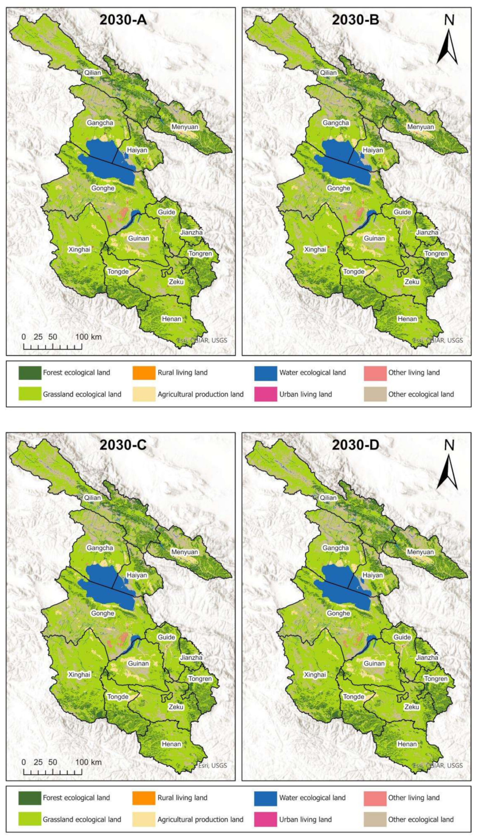
3.1. Scenario Prediction on PLE Land

PLE land in 2030 is generally similar to that in 2020 under the scenarios of natural growth (A) and cultivated land conservation (C). Production land is the smallest in the urban development scenario (B). Under the ecological protection scenario (D), the production and ecological land are the largest, while the living land is the smallest compared with other scenarios. Under the natural growth scenario, the production and living land increase slightly, while the ecological land decreases significantly, indicating human land use expansion (

Table 5. Comparison of PLE land each year/scenario (Unit: km²).

	2015	2020	2030A	2030B	2030C	2030D
Production	3493.3536	3479.1759	3491.1495	3461.9418	3491.154	3501.3375
Ecological	92,416.092	92,263.964	92,125.742	92,156.133	92,125.723	92,233.14
Living	190.5417	356.8473	482.0958	481.9131	483.111	365.5098

).

Under the urban development scenario, the production and ecological land decrease slightly, whereas the living land increases significantly. Under the cultivated land conservation scenario, the production land expands slightly, ecological land decreases slightly, and living land grows similarly to the first two scenarios, achieving the goal of protecting farmland. Under the ecological protection scenario, the production land increases slightly, while the living land increases less than in the previous three scenarios, and the ecological land loses slightly, but less than in 2020 (Table 5).

3.2. Scenario Prediction on PLE Sub-Land

In 2015, the Xining marginal area had 3493.35 km² of agricultural production land, 11,520.62 km² of forest ecological land, 59,935.19 km² of grassland ecological land, 6009.86 km² of water ecological land, 34.22 km² of urban living land, 128.65 km² of rural living land, 27.68 km² of other living land, and 14,950.42 km² of other ecological land. In contrast, the Xining marginal area in 2020 had 3479.18 km² (99.59% in 2015) of agricultural production land, 11,502.13 km² (99.84% in 2015) of forest ecological land, 59,706.83 km² (99.62% in 2015) of grassland ecological land, (103.14% in 2015) of water ecological land, 42.49 km² (124.19% in 2015) of urban living land, 133.85 km² (104.04% in 2015) of rural living land area, 180.51 km² (652.17% in 2015) of other living land, and 14,856.35 km² (99.37% in 2015) of other ecological land, as shown in Figure 3.

We simulated the evolution of the ecological–production–living land in 2030 by PLUS, and the ecological–production–living land in natural growth scenario (A), urban development scenario (B), cultivated land conservation scenario (C), and ecological protection scenario (D) is shown in Figure 4.

The natural growth scenario (scenario A) indicates a trend toward decreasing ecological land as compared to 2020, with the exception of an increase in the water ecological land in the counties of Haiyan, Gangcha, and Gonghe. While the other living land in Gonghe County has increased significantly, the living land and production land have only slightly increased. In the Xining marginal area, scenario A corresponds with an increase in land use without external interference.

The urban development scenario (scenario B) suggests that the production land decreases, with the highest decrease in Henan County, while the living land will expand overall, with Gonghe County experiencing the fastest growth in the other living land. Regarding the ecological land, the grassland ecological land in Haiyan, Gonghe, and Guinan Counties will be significantly decreased, as will the other ecological land also reduce. The water ecological land changes little; Haiyan County and Gonghe County have increased, whereas the forest ecological land will increase in general. The widespread expansion of the living land demonstrates the prioritization of urban development, which to some extent occupies the grassland ecological land.

Under the cultivated land conservation scenario (scenario C), the production land will grow minimally, whereas the agricultural production land in Gangcha and Gonghe Counties will grow more rapidly. The living land will also increase, with most of it occurring in Gonghe County. Except for the water ecological land, which will tend to increase, the remaining ecological land will decrease significantly. In this scenario, the goal of the cultivated land conservation is still not entirely achieved. In the ecological protection scenario (scenario D), the production land will grow minimally while the living land will remain largely unchanged. The grassland ecological land and other ecological land will decrease, while the forest ecological land and water ecological land will increase from 2020. Minor changes in the production and living lands, as well as the transition from the grassland ecological land and other ecological land to forest ecological land and water ecological land, demonstrate that conservation will on the top of the agenda in this scenario (

Table 6. Area and growth rate of each land use type compared to 2020.

	2015	2020	2030-A		2030-B		2030-C		2030-D
	Area	Area	Area	Rate	Area	Rate	Area	Rate	Area	Rate
b1	3493.35	3479.18	3491.15	0.34	3461.94	−0.50	3491.15	0.34	3501.34	0.64
b2	128.65	133.85	143.80	7.44	143.80	7.44	143.80	7.44	134.19	0.26
b3	34.32	42.49	49.22	15.84	51.48	21.15	49.28	15.97	41.97	−1.23
b4	11,520.62	11,502.13	11,471.60	−0.27	11,935.99	3.77	11,471.60	−0.27	11,957.16	3.96
b5	6009.86	6198.66	6331.42	2.14	6265.49	1.08	6330.24	2.12	6303.99	1.70
b6	59,935.19	59,706.83	59,504.39	−0.34	59,313.26	−0.66	59,504.63	−0.34	59,458.24	−0.42
b7	14,950.42	14,856.35	14,819.34	−0.25	14,641.39	−1.45	14,819.26	−0.25	14,513.76	−2.31
b8	27.68	180.51	289.08	60.14	286.64	58.79	290.04	60.67	189.35	4.90

Note: b1 refers to the agricultural production land, b2 refers to the rural living land, b3 refers to the urban living land, b4 refers to the forest ecological land, b5 refers to the water ecological land, b6 refers to the grassland ecological land, b7 refers to the other ecological land, and b8 refers to the other living land. The same applies below.

).

To summarize, the agricultural production land is predicted to increase by 2030, except for the urban growth scenarios. Except for the modest growth in the ecological protection scenario, the rural living land will increase at nearly the same rate (7.44%) in all the other scenarios. Except for the ecological protection scenario, all the scenarios predict an increase in the urban living land, with the urban development scenario showing the most significant growth rates. The other living land will also see significant expansion, with the ecological protection scenario indicating a slight increase and all the other scenarios exhibiting increases of about 60%. The forest ecological land will decrease slightly in the natural growth and cultivated land conservation scenarios while increasing in the urban development and ecological protection scenarios. The water ecological land is predicted to grow in all the scenarios, particularly in the natural growth and cultivated land conservation scenarios. All four scenarios will result in a decrease in the grassland ecological land, with urban development having the greatest effect. In all the scenarios, there will be decreases in the other ecological land, with the largest decrease in the ecological protection scenario.

3.3. Overall Pattern of Scenario Prediction on PLE Land in Each County

In the 2015, 2020, and 2030 scenarios, the land use in Xining’s marginal area is primarily production and ecological land, with a relatively low proportion of living land (about 0.1%). The grassland ecological land has the largest proportion, covering an area around 7–8 times that of production land, followed by the forest ecological land, which covers an area of 1.5–2 times that of production land. Specifically: (1) Forest ecological land is mainly distributed in Menyuan County, Tongren City, Jianzha County, and Tongde County, accounting for 20–22% of the total land use area of the counties. (2) Water ecological land is distributed relatively high in Haiyan County, Gangcha County, and Gonghe County. (3) Grassland ecological land accounts for a large proportion in all 14 counties, with the smallest proportion in Menyuan County, ranging from 38.14% to 39.37%. Except for Menyuan and Haiyan Counties, the proportion in all the other counties exceeds 50% of the total land use area, with Henan County having the highest at 79.01–79.77%. (4) Menyuan County, Qilian County, Haiyan County, Gangcha County, and Gonghe County are the counties with the highest proportions of other ecological land. (5) Menyuan, Tongde, Guide, and Guinan Counties contribute 8% to 12% of agricultural production land. (6) The proportions of rural living land, urban living land, and other living land in the 14 counties are quite low, with a total of approximately 1%, with only other living land in Gonghe County accounting for more than 0.1%. Figure 5 depicts the pattern of scenario predicted for each county’s PLE land in 2015, 2020, and 2030.

3.4. Core–Edge Mode on PLE Land in Xining Marginal Area

The Xining marginal area shows an evident core–edge pattern. We investigate the government seat as the core area (Haiyan County, Gonghe County, and Tongren City), and the remaining counties as external areas. The living land will increase overall, particularly the urban living land and other living land in the core areas, while the rural living land will see a similar growth rate. The agricultural production land will not grow significantly and may perhaps decrease in both the core and edge areas under scenario B. The grass ecological land and other ecological land may diminish more in the core areas under all the situations. Under scenarios A and C, the forest ecological land will decrease more in the core areas while under scenarios B and D, the core areas will witness more increase. The water ecological land will slightly increase in both the core and edge areas (

Table 7. Growth rate and core–edge mode of sub-land (%).

	2030-A		2030-B		2030-C		2030-D		Conclusion
	Core	Edge	Core	Edge	Core	Edge	Core	Edge
b1	0.455	0.316	−0.122	−0.591	0.454	0.316	0.439	0.688	all slightly increase except scenario B
b2	6.880	7.668	6.318	7.901	6.917	7.652	0.216	0.274	increase overall except scenario D
b3	36.658	8.292	43.500	13.050	36.705	8.457	0.016	−1.682	more growth in the core area
b4	−0.310	−0.254	5.504	3.316	−0.307	−0.255	5.535	3.541	varying according to the scenario
b5	2.745	1.352	1.808	0.123	2.715	1.348	1.272	2.258	all slightly increase
b6	−1.097	−0.120	−1.098	−0.532	−1.091	−0.121	−0.524	−0.385	all slightly decrease
b7	−1.109	0.082	−3.485	−0.663	−1.107	0.080	−2.878	−2.086	more decrease in the core area
b8	63.892	44.063	60.806	50.150	63.937	46.679	5.809	0.992	more growth in the core area

).

4. Spatial Optimization Strategies of PLE Land in Xining Marginal Area

4.1. Competitive Advantage Sets of PLE Land Under Each Scenario

The PFCI results trivialize the collection of competitive advantages in the sub-land in each scenario. Furthermore, the division of strong, weak, and non-competitive advantage sets influences the future direction of land use in the Xining marginal area (

Table 8. Competitive advantage sets of PLE land in different scenarios.

	Scenario A	Scenario B	Scenario C	Scenario D
Strong competitive set	{b6, b7}	{b6}	{b6, b7}	{b6, b7}
Weak competitive set	{b1, b5, b8}	{b1, b5, b7, b8}	{b1, b5, b8}	{b1, b2, b3, b5, b8}
Noncompetitive set	{b2, b3, b4}	{b2, b3, b4}	{b2, b3, b4}	{b4}

Note: Ranges of strong-, weak-, and non-conflict are [0.09, 1], [0.08, 0.09), and [0, 0.08), respectively. Scenario A means natural growth, scenario B means urban development, scenario C means cultivated land conservation, and scenario D means ecological protection.

).

The significant competitive advantage set consists mainly of the grassland ecological land (b6) and other ecological land (b7). This finding corresponds with the natural characteristics and endowments of the Xining marginal area; however, the other ecological land (b7) has a relatively low development value. As a result, focus should be on developing the grassland ecological land (b6).

The weak competitive advantage set mainly includes the agricultural production land (b1), water ecological land (b5), and other living land (b8). The agricultural production land is critical for guaranteeing regional food security while the water ecological land is basically invariable. The other living land (b8) is construction land, which includes road land, land for other units, reserved natural villages or unbuildable land, and so on. They have no development advantages in high-altitude, sparsely populated, and underdeveloped areas.

The non-advantage set mainly includes the rural living land (b2), urban living land (b3), and forest ecological land (b4), as the proportion of these types of land is relatively small, and they have no development advantages over the other land use types in the Xining marginal area. Among them, the urban living land (b3) shows a relatively clear spatial differentiation and the most dramatic changes, which make it worth being concerned about.

In Xining’s marginal area, the strong competitive advantage set is the grassland ecological land (b6), the weak competitive advantage set is the agricultural production land (b1), and the potential competitive advantage set is the urban living land (b3).

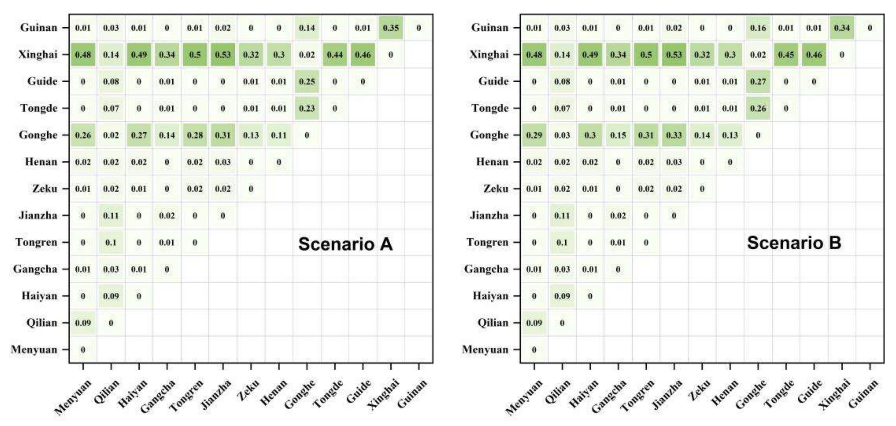
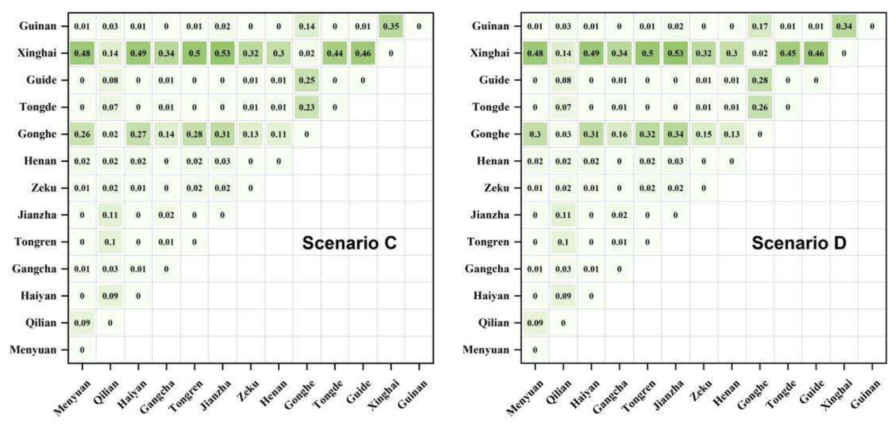
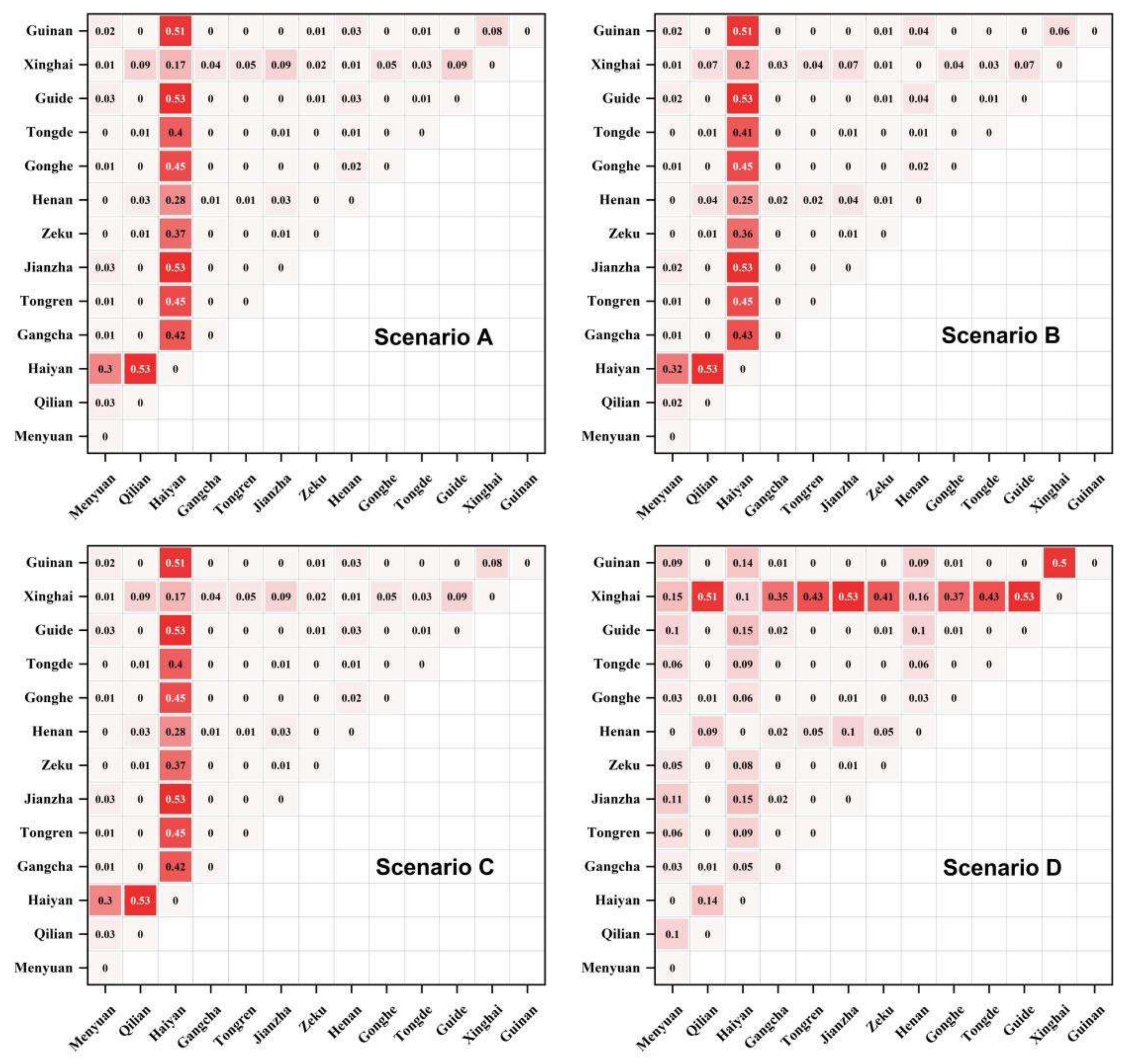
4.2. Competitive Advantage Sets between Counties

Conflicts between the different regions of the Xining marginal area range from 0 to 0.531 in every scenario. Based on the relative conflict values, we defined a strong conflict relation as [0.4, 0.531], a weak conflict relation as [0.2, 0.4), and a non-relative conflict relation as [0, 0.2).

(1)

Strong competitive advantage set: grassland ecological land (b6)

Xinghai County and Gonghe County are the primary sources of the grassland ecological land (b6) conflict, and they have the most influence in developing the grassland ecological land in all the scenarios. To be more specific, Xinghai County has a strong conflict relationship with Menyuan, Haiyan, Jianzha, Tongde, and Guide Counties, and Tongren City, but a weak conflict relationship with Gangcha, Zeku, Henan, and Guinan Counties. Gonghe County has weakdispute relationships with Menyuan, Haiyan, Jianzha, Tongde, and Guide Counties, and Tongren City (Figure 6). As a result, Xinghai and Gonghe Counties dominate in the development of the grassland ecological land.

(2)

Weak competitive advantage set: agricultural production land (b1)

Guinan County is the main area of the agricultural production land (b1) conflict. To be more specific, Guinan County has a major conflict with Qilian, Haiyan, Jianzha, Zeku, Henan, Guide, and Xinghai Counties, and Tongren City, as well as a weak conflict relationship with Gangcha and Tongde Counties (Figure 7). As a result, Guinan County dominates the development of the agricultural production land.

(3)

Potential competitive advantage set: urban living land (b3)

The urban living land (b3) may not have enough area to support the various forms of development, but as urbanization develops rapidly, its advantages will become more obvious. Additionally, it will become more crucial for regional development, appear to be a significant spatial conflict, and have a great deal of potential for economic development in the Xining marginal area. Haiyan County leads the development of the urban living land in the natural growth scenario (A), urban development scenario (B), and cultivated land conservation scenario (C), while Xinghai County dominates the development of the urban living land in the ecological protection scenario. Haiyan County has a significant conflict relationship with Qilian, Gangcha, Jianzha, Gonghe, Tongde, Guide, and Guinan Counties, and Tongren City, but a weak conflict relationship with Menyuan, Zeku, and Henan Counties. However, in the context of the ecological protection scenario, Xinghai County is the primary source of the urban living land conflict. Xinghai has strong conflict relationships with Qilian, Jianzha, Zeku, Tongde, Guide, and Guinan Counties, and Tongren City, but a weak conflict relationship with Gangcha and Gonghe Counties (Figure 8).

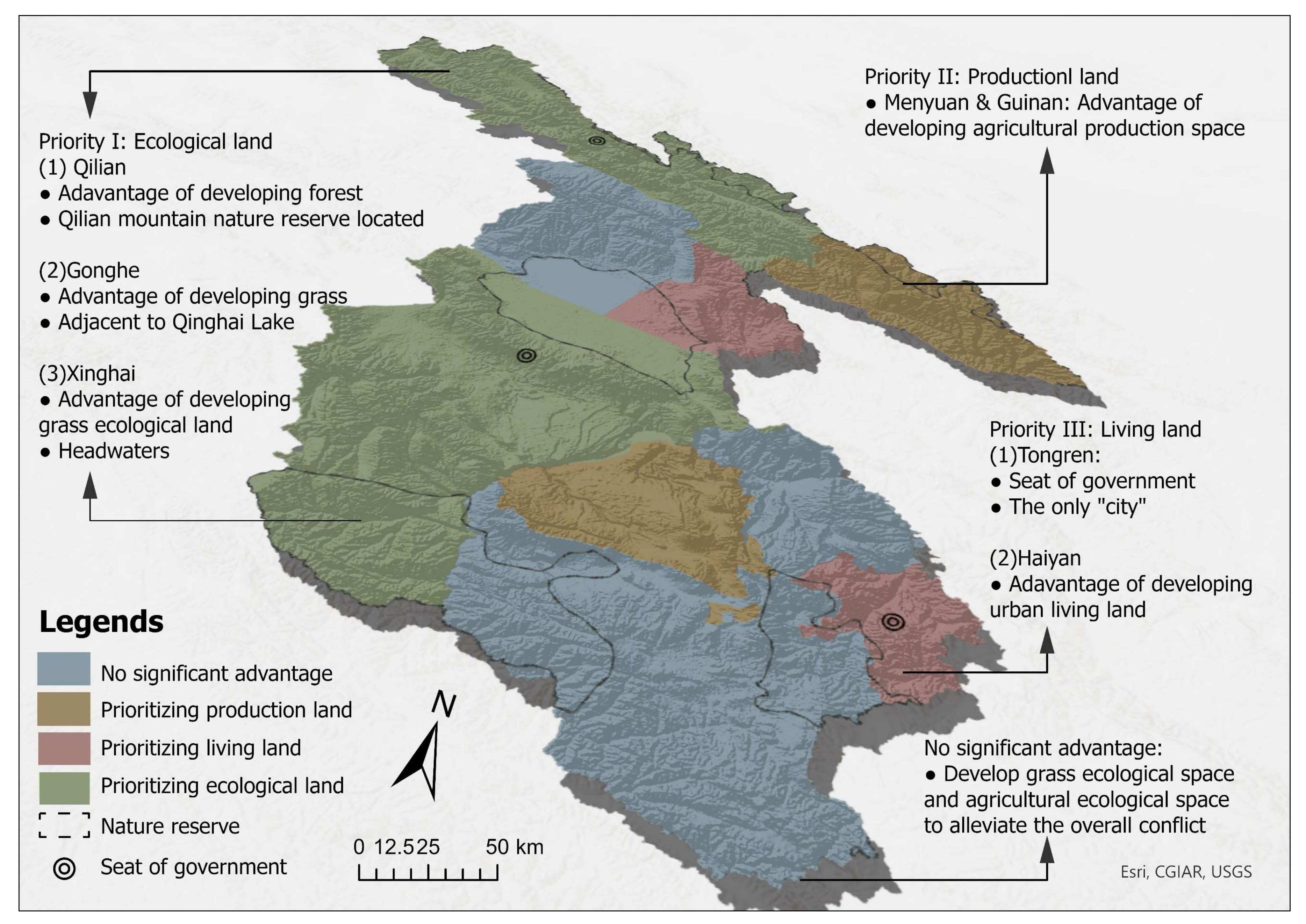
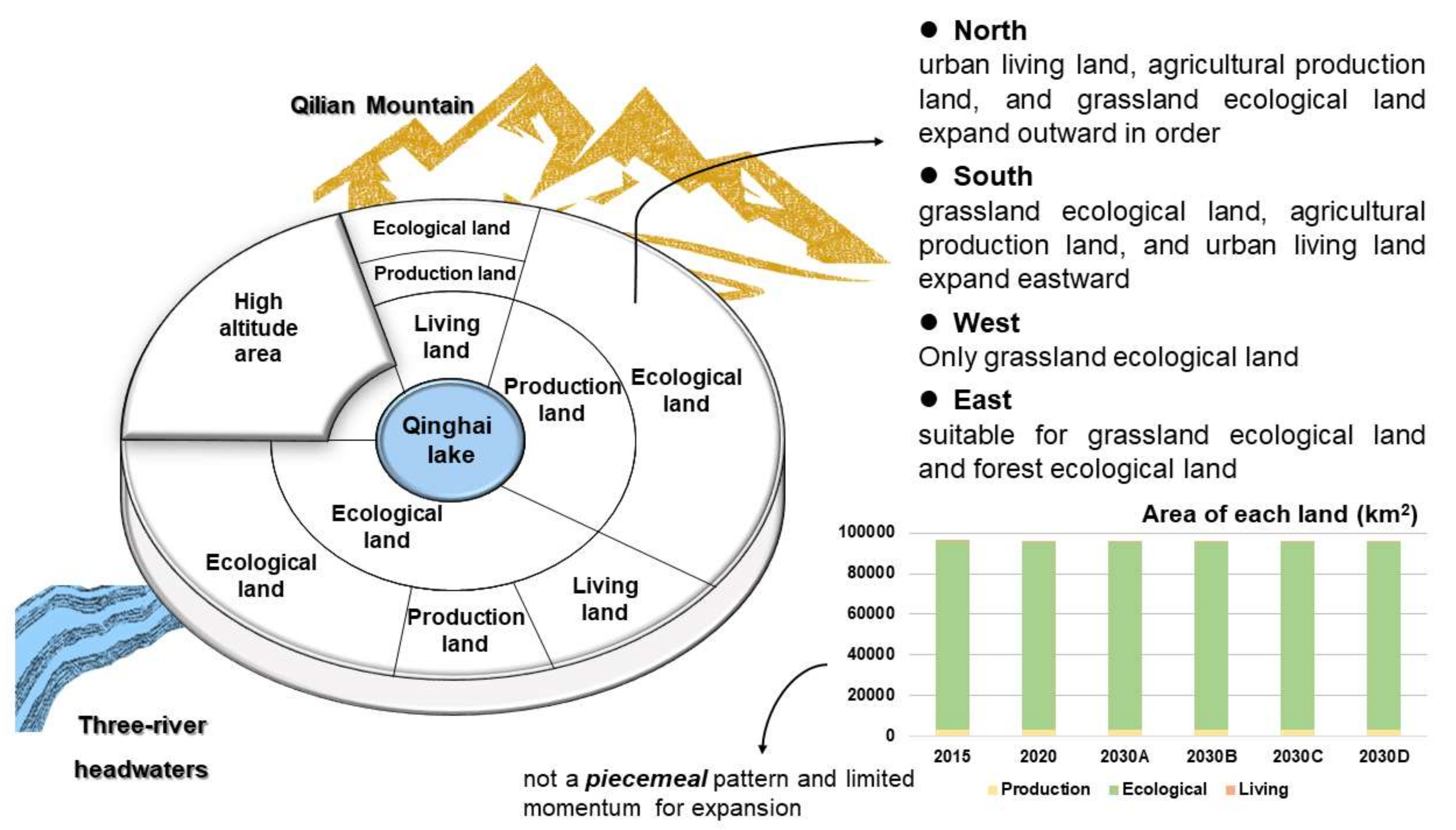
4.3. Spatial Distribution Optimization Strategies on PLE Land

Qinghai Province, as a plateau province, has complex terrain and an arid climate, but it also has abundant natural resources such as grassland and plateau lakes, providing conditions for the development of agriculture and animal husbandry. It is vital to consider factors such as land availability, resource endowment, and environmental protection to maximize the utilization of land resources and achieve optimal allocation. According to the PFCI, the Xining marginal area should develop the agricultural production land and grassland ecological land to effectively alleviate the overall conflicts. Therefore, as the periphery of the provincial capital, for the Xining marginal area, constrained by factors such as transportation and market, it is a better choice to develop agriculture and animal husbandry in the context of balancing economic development and environmental protection.

According to

Table 9. Sets of grassland ecological land.

X	A	B	C	D
L1	{L9, L12}	{L9, L12}	{L9, L12}	{L9, L12}
L2	{L12}	{L12}	{L12}	{L12}
L3	{L9, L12}	{L9, L12}	{L9, L12}	{L9, L12}
L4	{L9, L12}	{L9, L12}	{L9, L12}	{L9, L12}
L5	{L9, L12}	{L9, L12}	{L9, L12}	{L9, L12}
L6	{L9, L12}	{L9, L12}	{L9, L12}	{L9, L12}
L7	{ L12}	{L9, L12}	{L12}	{L9, L12}
L8	{L12}	{L12}	{L12}	{L12}
L9	{L1, L3, L4, L5, L6, L10, L11, L13}	{L1, L3, L4, L5, L6, L7, L10, L11, L13}	{L1, L3, L4, L5, L6, L10, L11, L13}	{L1, L3, L4, L5, L6, L7, L10, L11, L13}
L10	{L9, L12}	{L9, L12}	{L9, L12}	{L9, L12}
L11	{L9, L12}	{L9, L12}	{L9, L12}	{L9, L12}
L12	{L1, L2, L3, L4, L5, L6, L7, L8, L10, L11, L13}	{L1, L2, L3, L4, L5, L6, L7, L8, L10, L11, L13}	{L1, L2, L3, L4, L5, L6, L7, L8, L10, L11, L13}	{L1, L2, L3, L4, L5, L6, L7, L8, L10, L11, L13}
L13	{L9, L12}	{L9, L12}	{L9, L12}	{L9, L12}

Notes: (1) X means county/city, while L1 refers to Menyuan Hui Autonomous County, L2 refers to Qilian County, L3 refers to Haiyan County, L4 refers to Gangcha County, L5 refers to Tongren City, L6 refers to Jianzha County, L7 refers to Zeku County, L8 refers to Henan Mongol Autonomous County, L9 refers to Gonghe County, L10 refers to Tongde County, L11 refers to Guide County, L12 refers to Xinghai County, and L13 refers to Guinan County. The same applies below.

, in terms of the grassland ecological land, Gonghe County (L9) and Xinghai County (L12) are high-conflict areas, while Qilian County (L2) is a low-conflict area. Zeku County (L7) and Gonghe County (L9) differ from the other three scenarios only in terms of cultivated land protection, but the overall situation is very identical. As a result, developing the grassland ecological land is a top priority in Gonghe and Xinghai Counties, followed by Qilian County. Menyuan County (L1) and Guinan County (L13) are both high-conflict areas in terms of the agricultural production land, indicating that Menyuan and Guinan Counties should be prioritized for the agricultural production land development (

Table 10. Sets of agricultural production land.

X	A	B	C	D
L1	{L2, L5, L6, L8}	{L2, L5, L6, L8}	{L2, L5, L6, L8}	{L2, L5, L6, L8}
L2	{L1, L13}	{L1, L13}	{L1, L13}	{L1, L13}
L3	{L13}	{L13}	{L13}	{L13}
L4	{L13}	{L13}	{L13}	{L13}
L5	{L1, L13}	{L1, L13}	{L1, L13}	{L1, L13}
L6	{L1, L13}	{L1, L13}	{L1, L13}	{L1, L13}
L7	{L13}	{L13}	{L13}	{L13}
L8	{L1, L13}	{L1, L13}	{L1, L13}	{L1, L13}
L9	{L13}	{L13}	{L13}	{L13}
L10	{L13}	{L13}	{L13}	{L13}
L11	{L13}	{L13}	{L13}	{L13}
L12	{L13}	{L13}	{L13}	{L13}
L13	{L2, L3, L4, L5, L6, L7, L8, L9, L10, L11, L12}	{L2, L3, L4, L5, L6, L7, L8, L9, L10, L11, L12}	{L2, L3, L4, L5, L6, L7, L8, L9, L10, L11, L12}	{L2, L3, L4, L5, L6, L7, L8, L9, L10, L11, L12}

).

The strong competitive advantage sets of the urban living land (b3) in the natural growth scenario (A), urban development scenario (B), and cultivated land conservation scenario (C) show that Haiyan (L3) is a strong conflict area, while Xinghai County (L12) is a strong conflict area in the ecological protection scenario (D). Therefore, Haiyan County has advantages in developing the urban living land, which is followed by Xinghai County (

Table 11. Sets of urban living land.

X	A	B	C	D
L1	{L3}	{L3}	{L3}	{L12}
L2	{L3}	{L3}	{L3}	{L3, L12}
L3	{L1, L2, L4, L5, L6, L7, L8, L9, L10, L11, L12, L13}	{L1, L2, L4, L5, L6, L7, L8, L9, L10, L11, L12, L13}	{L1, L2, L4, L5, L6, L7, L8, L9, L10, L11, L12, L13}	{L2, L6, L11, L13}
L4	{L3}	{L3}	{L3}	{L12}
L5	{L3}	{L3}	{L3}	{L12}
L6	{L3}	{L3}	{L3}	{L3, L12}
L7	{L3}	{L3}	{L3}	{L12}
L8	{L3}	{L3}	{L3}	{L12}
L9	{L3}	{L3}	{L3}	{L12}
L10	{L3}	{L3}	{L3}	{L12}
L11	{L3}	{L3}	{L3}	{L3, L12}
L12	{L3}	{L3}	{L3}	{L1, L2, L4, L5, L6, L7, L8, L9, L10, L11, L12, L13}
L13	{L3}	{L3}	{L3}	{L3, L12}

).

5. Discussion and Conclusions

Qinghai, a plateau region with diverse topography and an arid climate, provides abundant grassland resources, plateau lakes, and other natural resources essential to agricultural and animal husbandry. The small population, poor natural environment, and restricted carrying capacity of the Xining marginal area have reduced the importance of expanding the urban and rural living land.

5.1. Discussion

By 2030, the Qinghai Tibet Plateau will not embark on the path of urbanization. The Xining marginal area is mostly used for production and ecological purposes, with a very small proportion of land designated for living and a unique core–edge pattern. The urban living land in the county where the government is located will increase more significantly, and the overall trend in PLE land is an increase in the living and production land, combined with a decrease in the ecological land, indicating that the Xining marginal area is still in the economic aggregation stage, but the relatively developed core areas have a limited impact on the other areas.

The development strategy of land use in the Xining Marginal area is significantly influenced by the natural environment. Overall, the counties and cities suitable for agricultural production land, grassland ecological land, and urban living land present a trend around the Qinghai Lake Basin at an altitude between 3000 and 3300 m. According to the PFCI, priority should be given to the development of the grassland ecological land in the counties of Gonghe and Xinghai, followed by Qilian County. Menyuan County and Guinan County should prioritize the development of the agricultural production land, followed by Gonghe County. Haiyan County has advantages in developing the urban living land in scenarios A, B, and C, followed by Xinghai County in scenario D. These counties are located around Qinghai Lake and can leverage their geographical advantages and resources to drive the development of agriculture, animal husbandry, and subsequently, the integrated development of secondary and tertiary industries.

From a county perspective, Haiyan and Gonghe Counties in the Qinghai Lake Basin have an absolute development advantage. Gonghe County surrounds Qinghai Lake on its east, south, and west sides, which is adjacent to the Three-river Headwaters National Nature Reserve and serves as the administrative center of Hainan Tibetan Autonomous Prefecture. It has comprehensive geographical development advantages and is suitable for the development of agricultural production land, grassland ecological land, and urban living land. The development of the grassland ecological land in this area has an absolute advantage in promoting ecological tourism around Qinghai Lake. Haiyan County, located northeast of Qinghai Lake, has abundant tourism resources. In recent years, with the impetus of urbanization and industrialization, there have been advantages in developing the urban living land. The majority of Gangcha is above 3300–3800 meters in altitude, and its development advantage is relatively weak.

The PLE land in the Xining Marginal area can be summarized by the following model. The PLE land does not exhibit a piecemeal expansion pattern, as it is influenced by mountains and rivers. The agricultural production land and grassland ecological land have advantages for development, whereas the urban living land has just development potential. Furthermore, the development pattern of the Qinghai Lake Basin exhibits a layered structure. The urban living land, agricultural production land, and grassland ecological land all expand outward in that sequence to the north of the Qinghai Lake Basin, with the Qilian Mountains forming the outermost circle. The urban living land, agricultural production land, and grassland ecological land all expand eastward to the south, constrained by the headwaters of three rivers. To the west of the Qinghai Lake Basin, only the development of the grassland ecological land is feasible at elevations above 3300 m. The Qilian Mountains, which are to the east, are suitable for the development of ecological lands with a grassland and forest ecological land (Figure 9).

Generally, the human–environment relationship system is essentially a complex system, and many global challenges are interconnected, and addressing only one aspect may exacerbate another. The intricate human–environment relationship system in the Xining Marginal area requires planners to reconcile the conflicts between traditional agricultural livelihoods and modern development, as well as the pressures of ecological environment protection and social development goals. This process involves multi-stakeholder models and cross-regional management, with the ultimate goal of enhancing human well-being. Similar issues exist in many regions of the Global South, particularly in areas that are impoverished, ecologically vulnerable, and in urgent need of social well-being enhancement, such as the Ganges River basin in India, the Amazon rainforest, and Southeast Africa.

This study provides ideas for sustainable development path design for these regions from three perspectives: land use prediction, land use interaction, and administrative unit interaction. It is essential to consider the future interactions between different spatial relationships and the competitive dynamics among different regional units. By adopting a zoning approach, strategically allocating advantageous land use types in favorable regions can promote regional sustainable development.

5.2. Nexus Approach for the Sustainable Development in Xining Marginal Area

Qinghai Province’s relatively slow economic development and uneven population distribution may result in development differences and competitiveness among different regions. Simultaneously, it is distinguished by a remote geographical location with inconvenient transportation, which may limit economic development. Whereas the National Territory Development Planning System requires the delineation of urban development boundaries to assure the spatial capacity of future urban development and construction, the arrangement of urban development time series results in a significant loss of rural development rights. In practice, local governments continue to implement indiscriminate policy supply for the region, and they are unable to timely change the system and policies that constrain the use of PLE land. The mismatch between policy supply and rural development stage will undoubtedly result in a decrease or even stagnation of the existing economies of scale, with the result that marginal areas will violate development laws. As a result, more specific and realistic actions must be implemented in the Xining marginal area to achieve a balance between economic development and environmental preservation.

The urbanization of the Qinghai–Tibet Plateau should be based on water tower protection and green development. Given the unique characteristics of plateau urbanization and the maximum permissible urban population size, the Qinghai–Tibet Plateau’s urbanization rate can be increased to 57.25%. Compared to the current urbanization rate of 47.58% in 2020, the Qinghai–Tibet Plateau may only expect a 9.67% increase in future urbanization [38]. Furthermore, the severe and fragile ecology of the Qinghai–Tibet Plateau necessitates a relatively small urban population. The plateau’s low carrying threshold prevents large-scale urbanization and development. The urbanization of the plateau does not conform to the law of stage development, and there is no need to significantly improve the urbanization of the plateau. Therefore, for counties with room to grow, urbanization can only take place at a low speed and with high quality.

The land use methods are designed to optimize the type and spatial combination of land use to protect land resources from damage; to gain the best integrated economic, social, and ecological benefits; and to maintain the long-term stability of such benefits [39]. We calculated the dominance of the different regions in developing different lands and designed a feasible nexus method for the sustainable development of the Xining marginal area (Figure 10). In this section, we propose five ways to reconcile the conflicts in the Xining marginal area, as shown below:

(1)

Low-speed development and high-quality urbanization

This approach applies to Haiyan County, Gonghe County, and Tongren City. According to Section 4.2, Haiyan County has dominance in developing urban living land, while Tongren City is a regional central city on the Qinghai–Tibet Plateau, acting as a point for driving social development and consolidating borders of the plateau [38]. In addition, according to Section 4.2, the living land in state government locations has a stronger growth momentum. Therefore, it is reasonable for Haiyan County and Tongren City to develop urban living lands. However, Gonghe County shows a diversity of appropriate characteristics. It has dominance in developing rural living land, other living land, and developing grassland ecological land. Therefore, it is worth exploring what type of lands Gonghe County should focus on constructing. We calculated the average conflict values of Gonghe County to develop the above lands under different scenarios. According to PFCI, in all the scenarios, Gonghe County has greater dominance in developing the rural living land and other living land, both of which are largely outside of the same competitive advantage set (see Section 4.2). Therefore, it is feasible for Gonghe County to focus on the rural living land and other living land based on its original foundation, with the grass ecological land surrounding it to protect the Qinghai Lake.

To conclude, Haiyan County, Gonghe County, and Tongren City are suitable for taking the approach of low-speed and high-quality urbanization. Fang also proposed to promote the conversion of Gonghe and Haiyan from counties into cities [38], which further verifies the views of this paper.

(2)

Mountain forest conservation

This approach applies to Qilian County. According to Section 4.3, Qilian County has dominance in developing forest ecological land and other ecological land. And given that the Qilian Mountain Nature Reserve lies in Qilian County, the path of mountain forest protection is advisable.

(3)

Plateau characteristic agriculture

This approach applies to Guinan and Menyuan, which have dominance in developing land for agricultural production. They should advocate the inheritance of traditional agricultural civilization and the moderate development of modern agriculture with highland characteristics on the premise of guaranteeing food security [40].

(4)

Water tower protection

This approach applies to Xinghai, Tongde, and Zeku Counties. Xinghai County has dominance in developing grassland ecological land. In addition, the unique alpine vegetation system in three-river headwaters plays a pivotal role in global climate change. The vegetation in the region determines the local ecology and animal husbandry production, and has a significant impact on the ecological security of China and Asia as a whole [41]. However, in the process of urbanization and industrialization in the three-river headwaters from 2012 to 2016, the environmental stress presented a point-like effect, the agricultural and animal husbandry production presented a planar stress, and the tourism and transportation presented a linear stress [42]. Therefore, the counties located in the three-river headwaters should take the approach of water town protection.

(5)

Live in town, pasture/farming in country

This approach applies to the counties characterized by no obvious dominance in development, including Gangcha, Guide, Jianzha, and Henan Counties. All these counties have a smaller center, surrounded by grassland ecological land or agricultural production land. According to Section 4.2, the development of grassland ecological land and agricultural production land may alleviate the overall conflict. It is appropriate for residents to live in the town, and pasture or farm in the country.

Figure 10. Nexus approaches for sustainable development of Xining marginal area.

Figure 10. Nexus approaches for sustainable development of Xining marginal area.

5.3. Limitations

Firstly, due to limitations in data acquisition and data volume, the influential factors we added to the PLUS model are not convincing enough. In addition, we only simulated the evolution pattern of the PLE lands in the different scenarios without specifying specific locations. For example, we did not add constrained areas or urban master plans to calculate the dominance of the development of different regions in the face of policy disruptions [43]. Secondly, due to the volume of data, we only considered the conflicts between the different lands from a holistic perspective, which was much larger in scale. We did not measure the conflicts between the different lands on a more microscopic scale, such as the spatial conflicts based on landscape ecology [44,45] or map multi-factor overlay [46,47].

5.4. Conclusions

In this study, we established the scenarios of natural growth, urban development, cultivated land conservation, and ecological protection based on the PLUS model, and calculated the competitive advantages between the different lands and regions in the Xining marginal area using PFCI. In conclusion, the Qinghai Tibet Plateau will not embark on the path of rapid urbanization by 2030. In any situation, the PLE land in the Xining marginal area is mainly focused on production and ecological land, with a very low proportion of living land (around 0.1%). The Xining marginal area has formed and will continue to maintain the core–edge pattern, namely, the seats of government will see stronger growth in the urban living land and other living land. All these indicate that the Xining marginal area is still in the early stages of economic development while the influence of the relatively developed areas exerted on other regions is still quite limited. The strong competitive advantage set includes the grassland ecological land and other ecological land, which indicates that in the Xining marginal area, the grassland ecological land and other ecological land have a dominant role or are in a dominant position. Regardless of the future development scenarios, the urban living land always plays a secondary role [47]. Gonghe County has dominance in developing rural living land and other living land, Xinghai County has dominance in developing grassland ecological land, Guinan County has dominance in developing agricultural production land, and Haiyan County has dominance in developing urban living land. On that basis, we analyzed the sustainable allocation strategies of the different lands and found that developing the corresponding lands in the dominant regions is the best option. Finally, we established nexus approaches to harmonizing conflicts for the Xining marginal area, aiming to provide a reference for the ecological highland. We hope that the Xining marginal area will thrive and become more lingering.

References

1. Hurtt, G.C.; Chini, L.P.; Frolking, S.; Betts, R.A.; Feddema, J.; Fischer, G.; Fisk, J.P.; Hibbard, K.; Houghton, R.A.; Janetos, A.; et al. Harmonization of land-use scenarios for the period 1500–2100: 600 years of global gridded annual land-use transitions, wood harvest, and resulting secondary lands. Clim. Chang. 2011, 109, 117–161. [Google Scholar] [CrossRef]
2. Haliscelik, E.; Soytas, M.A. Sustainable development from millennium 2015 to Sustainable Development Goals 2030. Sustain. Dev. 2019, 27, 545–572. [Google Scholar] [CrossRef]
3. Caiado, R.G.G.; Filho, W.L.; Quelhas, O.L.G.; Nascimento, D.L.d.M.; Ávila, L.V. A literature-based review on potentials and constraints in the implementation of the sustainable development goals. J. Clean. Prod. 2018, 198, 1276–1288. [Google Scholar] [CrossRef]
4. Lu, X.H.; Zhang, Y.W.; Lin, C.R.; Wu, F. Analysis and comprehensive evaluation of sustainable land use in China: Based on sustainable development goals framework. J. Clean. Prod. 2021, 310, 127205. [Google Scholar] [CrossRef]
5. Acheampong, M.; Yu, Q.Y.; Enomah, L.D.; Anchang, J.; Eduful, M. Land use/cover change in Ghana’s oil city: Assessing the impact of neoliberal economic policies and implications for sustainable development goal number one—A remote sensing and GIS approach. Land Use Policy 2018, 73, 373–384. [Google Scholar] [CrossRef]
6. Sun, H.L.; Zheng, D.; Yao, T.D.; Zhang, Y.L. Protection and Construction of the National Ecological Security Shelter Zone on Tibetan Plateau. Acta Geogr. Sin. 2012, 67, 3–12. [Google Scholar]
7. Han, W.; Cai, J.M.; Zhao, Y.F. Structure, mechanism, and paths of spatial governance in metropolitan fringe with the participation of multi-subjects. Prog. Geogr. 2021, 40, 1730–1745. [Google Scholar] [CrossRef]
8. Liao, G.; He, P.; Gao, X.; Lin, Z.; Huang, C.; Zhou, W.; Deng, O.; Xu, C.; Deng, L. Land use optimization of rural production–living–ecological land at different scales based on the BP–ANN and CLUE–S models. Ecol. Indic. 2022, 137, 108710. [Google Scholar] [CrossRef]
9. Cui, J.X.; Gu, J.; Sun, J.W.; Luo, J. The spatial pattern and evolution characteristics of the production, living and ecological space in Hubei provence. Chin. Land Sci. 2018, 32, 67–73. [Google Scholar]
10. Gao, L.A.; Tao, F.; Liu, R.; Wang, Z.L.; Leng, H.J.; Zhou, T. Multi-scenario simulation and ecological risk analysis of land use based on the PLUS model: A case study of Nanjing. Sustain. Cities Soc. 2022, 85, 104055. [Google Scholar] [CrossRef]
11. Reidsma, P.; Konig, H.J.; Feng, S.Y.; Bezlepkina, I.; Nesheim, I.; Bonin, M.; Sghaier, M.; Purushothaman, S.; Sieber, S.; Van, I.; et al. Methods and tools for integrated assessment of land use policies on sustainable development in developing countries. Land Use Policy 2011, 28, 604–617. [Google Scholar] [CrossRef]
12. Drechsler, M.; Surun, C. Land-use and species tipping points in a coupled ecological-economic model. Ecol. Complex. 2018, 36, 86–91. [Google Scholar] [CrossRef]
13. Hasegawa, T.; Fujimori, S.; Ito, A.; Takahashi, K.; Masui, T. Global land-use allocation model linked to an integrated assessment model. Sci. Total Environ. 2017, 580, 787–796. [Google Scholar] [CrossRef] [PubMed]
14. Verburg, P.H.; Tabeau, A.; Hatna, E. Assessing spatial uncertainties of land allocation using a scenario approach and sensitivity analysis: A study for land use in Europe. J. Environ. Manag. 2013, 127, 132–144. [Google Scholar] [CrossRef] [PubMed]
15. Chakir, R.; Le Gallo, J. Predicting land use allocation in France: A spatial panel data analysis. Ecol. Econ. 2013, 92, 114–125. [Google Scholar] [CrossRef]
16. Peltonen-Sainio, P.; Jauhiainen, L.; Laurila, H.; Sorvali, J.; Honkavaara, E.; Wittke, S.; Karjalainen, M.; Puttonen, E. Land use optimization tool for sustainable intensification of high-latitude agricultural systems. Land Use Policy 2019, 88, 104104. [Google Scholar] [CrossRef]
17. Sadeghi, S.H.R.; Jalili, K.; Nikkami, D. Land use optimization in watershed scale. Land Use Policy 2009, 26, 186–193. [Google Scholar] [CrossRef]
18. Arciniegas, G.; Janssen, R.; Omtzigt, N. Map-based multicriteria analysis to support interactive land use allocation. Int. J. Geogr. Inf. Sci. 2011, 25, 1931–1947. [Google Scholar] [CrossRef]
19. Kaim, A.; Cord, A.F.; Volk, M. A review of multi-criteria optimization techniques for agricultural land use allocation. Environ. Model. Softw. 2018, 105, 79–93. [Google Scholar] [CrossRef]
20. Rahman, M.M.; Szabo, G.A. Geospatial Approach to Measure Social Benefits in Urban Land Use Optimization Problem. Land 2021, 10, 1398. [Google Scholar] [CrossRef]
21. Zhao, X.; Tang, F.; Zhang, P.T.; Hu, B.Y.; Xu, L. Dynamic simulation and characteristic analysis of County production-living-ecological spatial conflicts based on CLUE-S model. Acta Ecol. Sin. 2019, 39, 5897–5908. [Google Scholar]
22. Gharaibeh, A.A.; Ali, M.H.; Abo-Hammour, Z.S.; Al Saaideh, M. Improving Genetic Algorithms for Optimal Land-Use Allocation. J. Urban Plan. Dev. 2021, 147, 04021049. [Google Scholar] [CrossRef]
23. Berger, T.; Schreinemachers, P. Creating agents and landscapes for multiagent systems from random samples. Ecol. Soc. 2006, 11, 19. [Google Scholar] [CrossRef]
24. Liang, X.; Guan, Q.F.; Clarke, K.C.; Liu, S.; Wang, B.Y.; Yao, Y. Understanding the drivers of sustainable land expansion using a patch-generating land use simulation (PLUS) model: A case study in Wuhan, China. Comput. Environ. Urban Syst. 2021, 85, 101569. [Google Scholar] [CrossRef]
25. Liu, X.P.; Liang, X.; Li, X.; Xu, X.C.; Ou, J.P.; Chen, Y.M.; Li, S.; Wang, S.; Pei, F. A future land use simulation model (FLUS) for simulating multiple land use scenarios by coupling human and natural effects. Landsc. Urban Plan. 2017, 168, 94–116. [Google Scholar] [CrossRef]
26. Liu, J.G.; Hull, V.; Godfray, H.C.J.; Tilman, D.; Gleick, P.; Hoff, H.; Pahl-Wostl, C.; Xu, Z.; Chung, M.G.; Sun, J.; et al. Nexus approaches to global sustainable development. Nat. Sustain. 2018, 1, 466–476. [Google Scholar] [CrossRef]
27. Flammini, A.; Puri, M.; Pluschke, L.; Dubois, O. Walking the nexus talk: Assessing the water-energy-food nexus in the context of the sustainable energy for all initiative. J. Phys. Chem. A 2014, 115, 7869–7870. [Google Scholar]
28. Rasul, G. Food, water, and energy security in South Asia: A nexus perspective from the Hindu Kush Himalayan region. Environ. Sci. Policy 2014, 39, 35–48. [Google Scholar] [CrossRef]
29. Shi, M.J.; Wu, H.Q.; Jiang, P.A.; Zheng, K.; Liu, Z.; Dong, T.; He, P.; Fan, X. Food-water-land-ecosystem nexus in typical Chinese dryland under different future scenarios. Sci. Total Environ. 2023, 880, 163183. [Google Scholar] [CrossRef]
30. He, X.H. Analysis on Land Use Structure of Ecological-production-living land in Shaanxi Province. Remote Sens. Inf. 2021, 36, 120–124. [Google Scholar]
31. Li, G.D.; Fang, C.L. Quantitative function identification and analysis of urban ecological-production-living lands. Acta Geogr. Sin. 2016, 71, 49–65. [Google Scholar]
32. Liu, J.L.; Liu, Y.S.; Li, Y.R. Classification evaluation and spatial-temporal analysis of “production-living-ecological” lands in China. Acta Geogr. Sin. 2017, 72, 1290–1304. [Google Scholar]
33. Zhang, H.Q.; Xu, E.Q.; Zhu, H.Y. An ecological-living-industrial land classification system and its spatial distribution in China. Resour. Sci. 2015, 37, 1332–1338. [Google Scholar]
34. Wang, J.N.; Zhang, Z. Land Use Change and Simulation Analysis in the Northern Margin of the Qaidam Basin Based on Markov-PLUS Model. J. Northwest For. Univ. 2022, 37, 139–148. [Google Scholar]
35. Wang, B.S.; Liao, J.F.; Zhu, W.; Qiu, Q.Y.; Wang, L.; Tang, L. The weight of neighborhood setting of the FLUS model based on a historical scenario: A case study of land use simulation of urban agglomeration of the Golden Triangle of Southern Fujian in 2030. Acta Ecol. Sin. 2019, 39, 4284–4298. [Google Scholar]
36. Zadeh, L.A. Fuzzy sets. Inf. Control. 1965, 8, 338–353. [Google Scholar] [CrossRef]
37. Yager, R.R. Pythagorean Membership Grades in Multicriteria Decision Making. IEEE Trans. Fuzzy Syst. 2014, 22, 958–965. [Google Scholar] [CrossRef]
38. Fang, C.L. Special thinking and green development path of urbanization in Qinghai-Tibet Plateau. Acta Geogr. Sin. 2022, 77, 1907–1919. [Google Scholar]
39. Giuliani, G.; Mazzetti, P.; Santoro, M.; Nativi, S.; Van Bemmelen, J.; Colangeli, G.; Lehmann, A. Knowledge generation using satellite earth observations to support sustainable development goals (SDG): A use case on Land degradation. Int. J. Appl. Earth Obs. Geoinf. 2020, 88, 102068. [Google Scholar] [CrossRef]
40. Liu, Y.S.; Zhang, Z.W.; Wang, J.Y. Regional differentiation and comprehensive regionalization scheme of modern agriculture in China. Acta Geogr. Sin. 2018, 73, 203–218. [Google Scholar]
41. Li, H.X.; Liu, G.H.; Fo, B.J. Response of vegetation to climate change and human activity based on NDVI in the Three-River Headwaters region. Acta Ecol. Sin. 2011, 31, 5495–5504. [Google Scholar]
42. Zhou, K.; Liu, H.C.; Fan, J.; Yu, H. Environmental stress intensity of human activities and its spatial effects in the Qinghai-Tibet Plateau national park cluster: A case study in Sanjiangyuan region. Acta Ecol. Sin. 2021, 41, 268–279. [Google Scholar]
43. Zhou, L.; Dang, X.W.; Sun, Q.K.; Wang, S.H. Multi-scenario simulation of urban land change in Shanghai by random forest and CA-Markov model. Sustain. Cities Soc. 2020, 55, 102045. [Google Scholar] [CrossRef]
44. Bao, W.K.; Yang, Y.Y.; Zou, L.L. How to reconcile land use conflicts in mega urban agglomeration? A scenario-based study in the Beijing-Tianjin-Hebei region, China. J. Environ. Manag. 2021, 296, 113168. [Google Scholar] [CrossRef] [PubMed]
45. Jiang, S.; Meng, J.J.; Zhu, L.K.; Cheng, H.R. Spatial-temporal pattern of land use conflict in China and its multilevel driving mechanisms. Sci. Total Environ. 2021, 801, 149697. [Google Scholar] [CrossRef] [PubMed]
46. Zou, L.L.; Liu, Y.S.; Wang, J.Y.; Yang, Y.Y. An analysis of land use conflict potentials based on ecological-production-living function in the southeast coastal area of China. Ecol. Indic. 2021, 122, 107297. [Google Scholar] [CrossRef]
47. Jiang, S.; Meng, J.J.; Zhu, L.K. Spatial and temporal analyses of potential land use conflict under the constraints of water resources in the middle reaches of the Heihe River. Land Use Policy 2020, 97, 104773. [Google Scholar] [CrossRef]
Figure 1. Position of Xining marginal area.
Land 13 01241 g001
Figure 2. Flowchart of the research.
Land 13 01241 g002
Figure 3. Distribution of different lands in 2015 and 2020.
Land 13 01241 g003
Figure 4. Distribution of different lands under 2030 scenarios.
Land 13 01241 g004
Figure 5. Patterns of scenario prediction on PLE land of each county. Note: scenario A means natural growth, scenario B means urban development, scenario C means cultivated land conservation, and scenario D means ecological protection.
Land 13 01241 g005
Figure 6. Relative conflict of grassland ecological land between different regions. Note: Scenario A means natural growth, scenario B means urban development, scenario C means cultivated land conservation, and scenario D means ecological protection.
Land 13 01241 g006aLand 13 01241 g006b
Figure 7. Relative conflict of agricultural production land between different regions. Note: Scenario A means natural growth, scenario B means urban development, scenario C means cultivated land conservation, and scenario D means ecological protection.
Land 13 01241 g007
Figure 8. Relative conflict of urban living land between different regions. Note: Scenario A means natural growth, scenario B means urban development, scenario C means cultivated land conservation, and scenario D means ecological protection.
Land 13 01241 g008
Figure 9. Layered structure of PLE land in Xining marginal area.
Land 13 01241 g009