Article

Investigating the Nonlinear Effect of Land Use and Built Environment on Public Transportation Choice Using a Machine Learning Approach

1
School of Architecture and Art, Hebei University of Engineering, Handan 056038, China
2
School of Architecture, Tianjin University, Tianjin 300072, China
*
Author to whom correspondence should be addressed.
Land 2024, 13(8), 1302; https://doi.org/10.3390/land13081302
Submission received: 29 June 2024 / Revised: 10 August 2024 / Accepted: 14 August 2024 / Published: 16 August 2024
(This article belongs to the Special Issue GeoAI for Urban Sustainability Monitoring and Analysis)

Abstract

:
Understanding the relationship between the demand for public transportation and land use is critical to promoting public-transportation-oriented urban development. Taking Beijing as an example, we took the Public Transportation Index (PTI) during the working day’s early peak hours as the dependent variable. And 15 land use and built environment variables were selected as the independent variables according to the “7D” built environment dimensions. According to the Modifiable Areal Unit Problem (MAUP), the size and shape of the spatial units will affect the aggregation results of the dependent variable and the independent variables. To find the ideal spatial unit division method, we assess how well the nonlinear model fits several spatial units. Extreme Gradient Boosting (XGBoost) was utilized to investigate the nonlinear effects of the built environment on PTI and threshold effects based on the ideal spatial unit. The results show that (1) the best spatial unit division method is based on traffic analysis zones (TAZs); (2) the top four explanatory variables affecting PTI are, in order: mean travel distance, residential density, subway station density, and public services density; (3) there are nonlinear relationships and significant threshold effects between the land use variables and PTI. The priority regeneration TAZs were identified according to the intersection analysis of the low PTI TAZs set and the PTI-sensitive TAZs set based on different land use variables. Prioritized urban regeneration TAZs require targeted strategies, and the results of the study may provide a scientific basis for proposing strategies to renew land use to increase PTI.

1. Introduction

The unlimited growth of cities has led to a rapid increase in the number of private cars, which in turn has led to increased traffic congestion and air pollution [1]. To alleviate traffic congestion and deteriorating air quality, the government encourages residents to use buses and subways as their preferred mode of transport [2]. Public transportation, as an intensive, green, and sustainable mode of transport development, is an effective way to relieve urban traffic congestion and implement China’s goal of “carbon peaking by 2030 and carbon neutrality by 2060”.
In just 30 years, Beijing has developed rapidly. But at the same time, transport problems and conflicts have become more and more obvious. The results of Beijing’s fifth comprehensive traffic survey show that for the first time, the proportion of car trips has dropped, and the proportion of public transport trips has risen. It has been demonstrated that policymakers’ forecast of the demand for public transportation is crucial to the long-term viability of public transportation [3]. Therefore, analyzing the factors affecting the demand for public transportation is conducive to the healthy development of Beijing’s public transportation system.
In terms of data sources, most existing studies use questionnaires or censuses to obtain travel data. The data are still manually obtained, not updated in time, and not open-source data, which has significant limitations [4,5,6,7]. Multi-source data are now characterized by full samples. Calculating the proportion of transit mode trips requires the use of other transport mode trip record data. However, it is difficult to obtain a full sample of data on private cars, walking, and cycling. Data on bus Intelligent Card (IC) payments and other modes of payment provide real and comprehensive data to study the demand for travel by public transportation modes. The ratio of IC card payments for public transportation to the population can be used to reflect the actual demand of the population in the region. This ratio, known as the Public Transportation Index (PTI) [8], is used to reflect the proportion of residents choosing public transportation. We used the number of IC card payments for public transportation in Beijing to calculate the number of public transportation trips and cell phone data to analyze the number of residents in the units, which has stronger timeliness and accuracy than traditional data acquisition methods [9].
The public transportation system is an important part of the city’s operating system, and the factors affecting the demand for public transportation are complex [8,10]. At first, scholars focused on the effects of green coverage rates [11], land use diversity [12,13], and the age of the population [14] on the demand for public transportation. With the continuous development and renewal of cities, academics are starting to focus on how certain aspects of the built environment affect the demand for public transportation, such as traffic, urban design, and the density of various types of facilities [15], but a more comprehensive analysis of built environment variables is lacking. On the basis of the “3D” dimensions proposed by Handy [16], namely, density, diversity, and design, Ewing et al. added two factors, namely distance to transit and destination accessibility, and proposed the “5D” dimensions [17]. Then, Ewing et al. added demand management and demographics based on “5D” to form “7D” dimensions [18], making the dimensions of the built environment richer. At present, most scholars mainly use the “5D” dimensions to explore the impact of the built environment variables on the demand for public transportation [8,9,19].
Differences in the aggregation of public transportation demand and built environment can affect the analysis results [20]. Dividing the aggregation unit is the first stage in many geographical problem study projects [21]. Openshaw describes this phenomenon as the Modifiable Area Unit Problem (MAUP), which refers to the problem that the analysis results vary with the definition of units [20]. There are two components in the MAUP. One is the scale effect, that is, different area unit sizes [22]; the other is the zoning effect, that is, different shapes of unit elements, such as square grids [23], traffic analysis zones [24,25,26], Voronoi diagrams [24,27,28,29,30], zip codes [31,32], etc. Existing studies have mostly empirically determined the scale and shape of the spatial units [33,34], and few studies have relied on comparing the results of quantitative analyses of different spatial units.
In terms of modeling methods, ordinary least squares (OLS), structural equation modeling (SEM), geographically weighted regression (GWR), geographically and temporally weighted regression (GTWR), and other models are often used in research on the impact of the built environment on public transportation demand [9,35,36]. Compared to traditional linear regression models, machine learning has no pre-assumptions. Machine learning provides more accurate predictions and is a superior model choice for exploring complex nonlinear relationships [37]. XGBoost is one of the machine learning models that has many advantages over other machine learning models such as random forest [38,39,40] and deep learning [41]: it prevents overfitting, suits small datasets, reflects threshold effects, unifies global and single-sample explanations, is immune to multicollinearity, can explore factor interactions, etc. [42,43]. XGBoost is now widely used in the fields of disaster prediction [44,45], infectious disease prediction [46], smart cities [47,48], commuting by walking [49], remote sensing image processing [50], etc. However, it has been less applied in the study of factors influencing the proportion of public transportation trips. The dynamics and spatial heterogeneity of public transportation lead to a spatial imbalance of factors affecting PTI [51], and we chose XGBoost to better explore the complex nonlinear relationship between land use and PTI. Its nonlinear threshold effect can identify the right range or threshold, which can be cost-effective and help urban planners create more accurate land use renewal plans to achieve higher public transportation shares in different areas [49,52]. To our knowledge, few studies have analyzed the threshold effects of influencing factors on traffic travel behavior, although Tao and Cao [53] analyzed the thresholds of built environment variables associated with driving distance, transit distance, and active travel distance.
To fill the gaps, this study investigated how land use and the built environment affected PTI. The optimal spatial unit was found using XGBoost, and the nonlinear and threshold effects of land use on PTI were investigated. This research has three main objectives:
(1)
Compare the goodness of model fitting for different scale grids, TAZs, and neighborhoods as spatial units and identify the optimal spatial unit.
(2)
Explore the extent to which the land use and built environment variables affect the PTI based on the optimal spatial unit.
(3)
XGBoost was used to explore the nonlinear relationship and threshold effect of land use variables on PTI. The spatial units with priority renewal will be identified based on research findings.

2. Data Sources and Methods

2.1. Overview of the Study Area and Data Sources

The study region was chosen to be within Beijing’s 6th Ring Road (Figure 1). The study area covers an area of about 2267 KM2 and has a resident population of 14 million. The dependent variable in this study was derived from public transportation card payment data for five weekdays from 12 October 2020 to 16 October 2020. The processed trip record data contain the field information shown in Table 1. Public transportation includes bus and subway modes. We omit the possible transfer behavior of travelers during a trip, such as first taking a bus line to the subway station and then transferring to another subway line to the destination. We believe that the omitted information does not affect the analysis of the Public Transportation Index (PTI).

2.2. Methods

2.2.1. The Public Transportation Index

In order to better reflect and predict the demand for public transportation in different units, we use the Public Transportation Index (PTI) proposed by Liu et al. as an indicator to measure regional public transportation demand [8], which is calculated using Equation (1).
P T I i = V i R i
where Vi is the number of public transportation boardings within the spatial unit i during the working day’s early peak hours, and Ri is the population within the spatial unit i. An increased PTI number signifies a greater proportion of the populace that utilizes public transportation. Therefore, a higher PTI value represents a higher demand or attraction for the public transportation mode.

2.2.2. XGBoost

XGBoost has good modeling ability for nonlinear features of various types of data. XGBoost is used to study the nonlinear relationship between land use and PTI, which is calculated using Equation (2):
y ^ l ( d ) = y ^ l ( d 1 ) + f d ( x q )
where y ^ l ( d ) is the lth spatial unit’s PTI predicted by the model after the dth round of iterations; y ^ l ( d 1 ) is the predicted value of the known set of d − 1 decision trees; f d ( x q ) is the dth decision tree; and x q is the qth land use explanatory variable. The core of the XGBoost model solution is to fit the residuals of the d − 1th decision tree to the dth decision tree and calculate the results of all decision trees after reaching the number of iterations.

2.2.3. Explanation of Machine Learning Models: SHAP (Shapley Additive Explanations)

Lundberg and Lee proposed Shapley Additive Explanations (SHAP) in 2018 [54], which identifies global and local effects. It can bridge the gap between the accuracy and interpretability of machine learning models’ predictions.
A Shapley value is calculated using Equation (3):
θ p = s { x 1 , x p } \ { x p } | s | ! ( | p | | s | 1 ) ! | p | ! ( f ( s { x p } ) f ( s ) )
where θ p is the Shapley value of variable P, S is a subset of the features incorporated into the model, x p is the value vector of variable P, and P is the number of the ith variables. f ( s ) is the prediction for variable values in set S.

2.3. Land Use Explanatory Variables

Combined with the relevant foreign theoretical studies, 15 land use and built environment explanatory variables (Table 2) were selected based on the “7D” dimensions. Among them, diversity represents the distribution of different types of land within a certain range and the diversity of business forms. Therefore, Shannon’s diversity index was selected to calculate the land use mixing degree [55]. Four indicators were chosen to measure the distance to transit: public transportation network density, bus station density, subway station density, and vertical distance from the bus stop to the nearest primary road or trunk road. In previous studies, destination accessibility was measured by the distance to the central business district (CBD). But, for the mega-city Beijing, there are multiple CBDs. This research measures destination accessibility by the mean travel distance of public transportation trips whose origin stations are within the spatial unit.

3. Results and Discussion

3.1. Optimal Scale and Shape of the Spatial Unit

Figure 2 shows the different methods of dividing spatial units. We selected square grids from 200 m to 2000 m (interval 100 m), TAZ, and neighborhood as the spatial units. In the process of XGBoost model training and testing, grid search and 5-fold cross-validation were used to optimize the parameters of the XGBoost regression model to prevent overfitting and improve the model’s prediction accuracy. The mean absolute error (MAE), mean square error (MSE), mean absolute percentage error (MAPE), root mean square error (RMSE), and R2 comparison results of the testing dataset of XGBoost for different spatial units are shown in Table 3. The comparison found that using TAZ as the spatial unit had the highest R2. The higher the R2, the better the model fit. So, TAZ is the optimal spatial unit of this study. For the XGBoost model under the TAZ spatial unit, the optimal parameters are as follows: max_depth is 9, learning_rate is 0.02, subsample is 0.34, colsample_bytree is 0.79, n_estimators is 5626, and gamma is 5.25. The PTIs of TAZs were spatially classified into three categories: low, middle, and high by using the ArcGIS natural breaks classification (Jenks) toolbox, as shown in Figure 3.

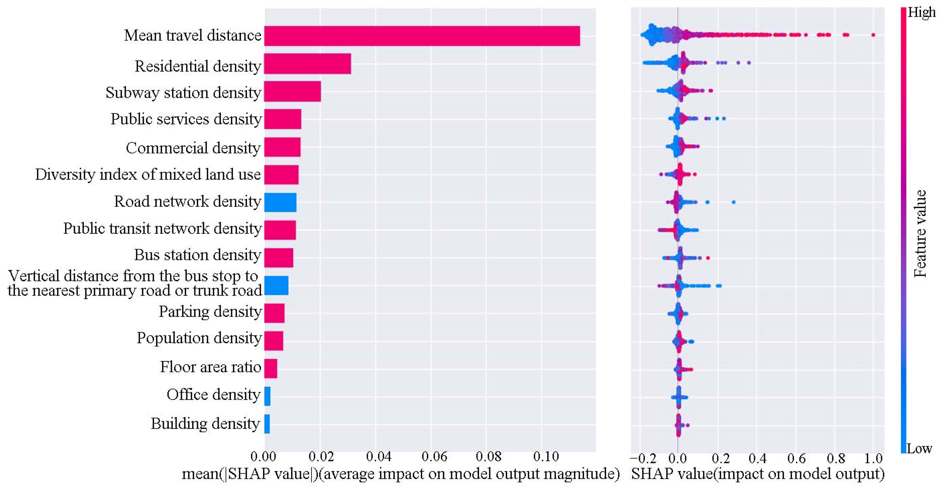
3.2. Global Impact of Explanatory Variables on PTI

The SHAP values can help reveal nonlinear relationships and determine the relative importance of explanatory variables in the prediction [57,58]. Figure 4 displays the average SHAP values of the explanatory variables for PTI, with global positive correlations shown in warm colors and global negative correlations in cool colors. The explanatory variables that contribute to PTI are, in descending order, mean travel distance, residential density, subway station density, public services density, commercial density, diversity index of mixed land use, roadway network density, public transportation network density, bus station density, the vertical distance from the bus stop to the nearest primary road or trunk road, parking density, population density, floor area ratio, office density, and building density. Among them, mean travel distance contributes the most to PTI. The further the mean travel distance, the more residents tend to choose public transportation. This may be due to the fact that walking and biking are time-consuming, while driving cars faces severe road congestion and high parking charges. Public transportation survey results have shown that 39.7% of the population living between the Fifth Ring Road and the Sixth Ring Road have a commute time of more than 45 min. The urban layout, characterized by the separation of jobs and residences, has led to high time consumption and long-distance commuting [59], making public transportation the preferred mode of travel. The second most influential explanatory variable is residential density. The reason may be that the higher the residential density, the more crowded the car travel, and people are more willing to choose public transportation. The third important explanatory variable is the density of subway stations. The reason is that the greater the number of subway stations in these TAZs, the more commuters prefer to choose the on-time and fast subway as a travel mode.
Variables that are globally negatively correlated with PTI are road network density, vertical distance from the bus stop to the nearest primary road or trunk road, office density, and building density. The reason for the negative correlation between road density and PTI may be that the higher the road density in spatial units, the more convenient it is for residents to travel by walking or biking, making them less likely to choose public transportation. The vertical distance from the bus stop to the nearest primary road or trunk road is negatively correlated with PTI for the obvious reason that the smaller the vertical distance, the more convenient it is for residents to choose public transportation mode, especially express bus lines along the primary road or trunk road. In TAZs with high parking density, it is more convenient for residents to park, and the proportion of the population choosing public transportation is relatively low. The reason for the negative correlation between office density and PTI may be that commuters choosing public transportation tend to live in outlying areas of the city, while employment is concentrated in several core areas of the city. As a result, TAZs with high office density generate relatively few public transportation trips during the morning peak hours.
Since Beijing has a multi-center urban structure with employment centers scattered in multiple areas, we did not use the variable distance to the city center. The mean travel distance is the average Manhattan distance of all public transportation trips originating within a TAZ, which can indicate accessibility and convenience to destinations. Our results show that the mean travel distance is the most important factor affecting PTI, which is similar to the results of Tao and Cao [53]. They concluded that the three most important variables affecting bus travel distance are, in order, job accessibility, distance to St. Paul, and distance to Minneapolis. For Beijing, the longer the travel distance, the more likely people are to choose public transportation. Therefore, for those TAZs with longer mean travel distances, urban planners should pay attention to providing direct and convenient public transportation routes planning services.

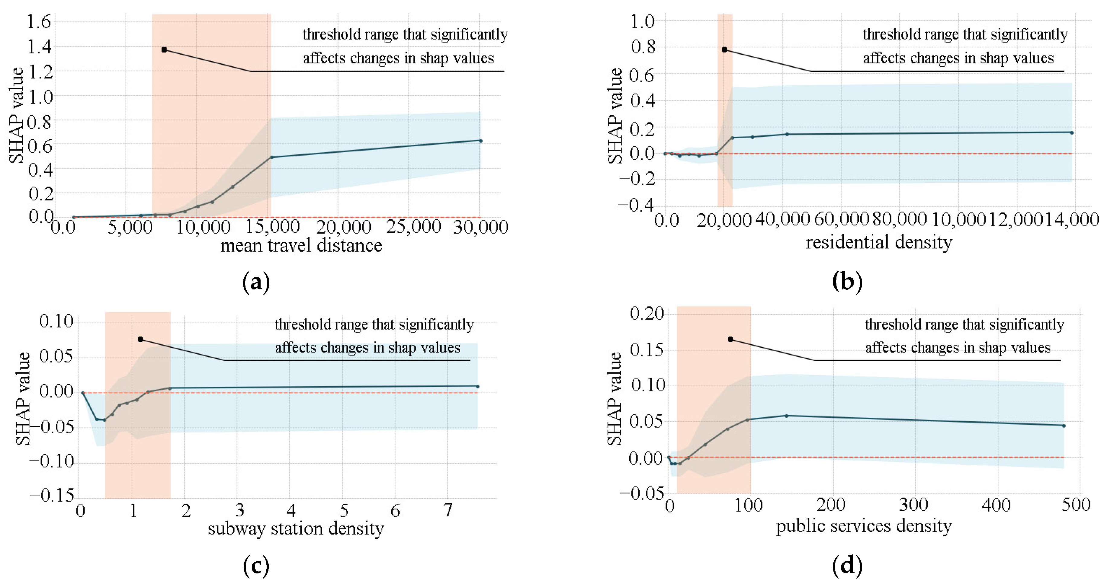
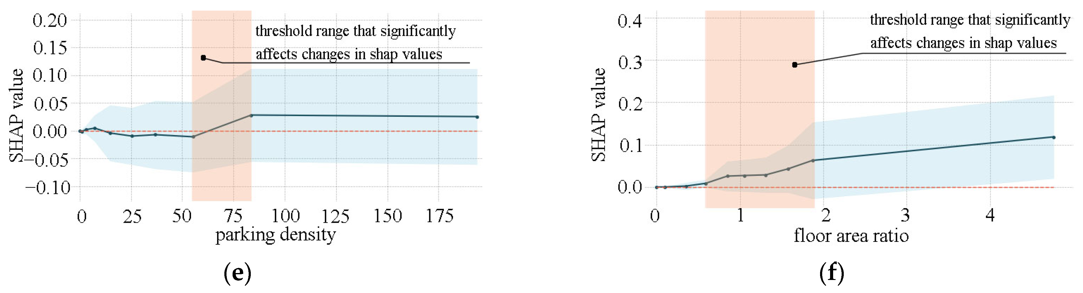
3.3. Analysis of Nonlinear Relationships in Land Use

Figure 5 illustrates the nonlinear relationships between land use and PTI. We chose six land use variables for nonlinear analysis, and these six variables are relatively easy to implement during the built environment updating process. The nonlinear relationships between other variables and PTI are shown in Figure S1. Overall, all explanatory variables had relatively complex nonlinear relationships and threshold effects with PTI. The threshold effect indicates that the slope of SHAP value change of a variable is steeper in this interval range, which means that the variable has a stronger influence on the dependent variable PTI when it is in this interval range. Tao and Cao [53] also pointed out that threshold ranges effectively alter travel distances. Figure 5a demonstrates the global positive correlation between mean travel distance and PTI, and there is a clear threshold effect. When the mean travel distance is between 7 and 15 km, PTI increases rapidly with the increase in mean travel distance. This range of values (7–15 km) is called the threshold range that significantly affects SHAP values. Figure 5b demonstrates the global positive correlation between residential density and PTI, which is consistent with the results of existing studies [60], with a significant threshold range between 20,000 and 25,000 person/km2. Figure 5d–f illustrate the nonlinear relationships between subway station density, public services density, parking density, floor area ratio, and PTI, respectively. The threshold range that significantly affects SHAP values is also shown in Figure 5.

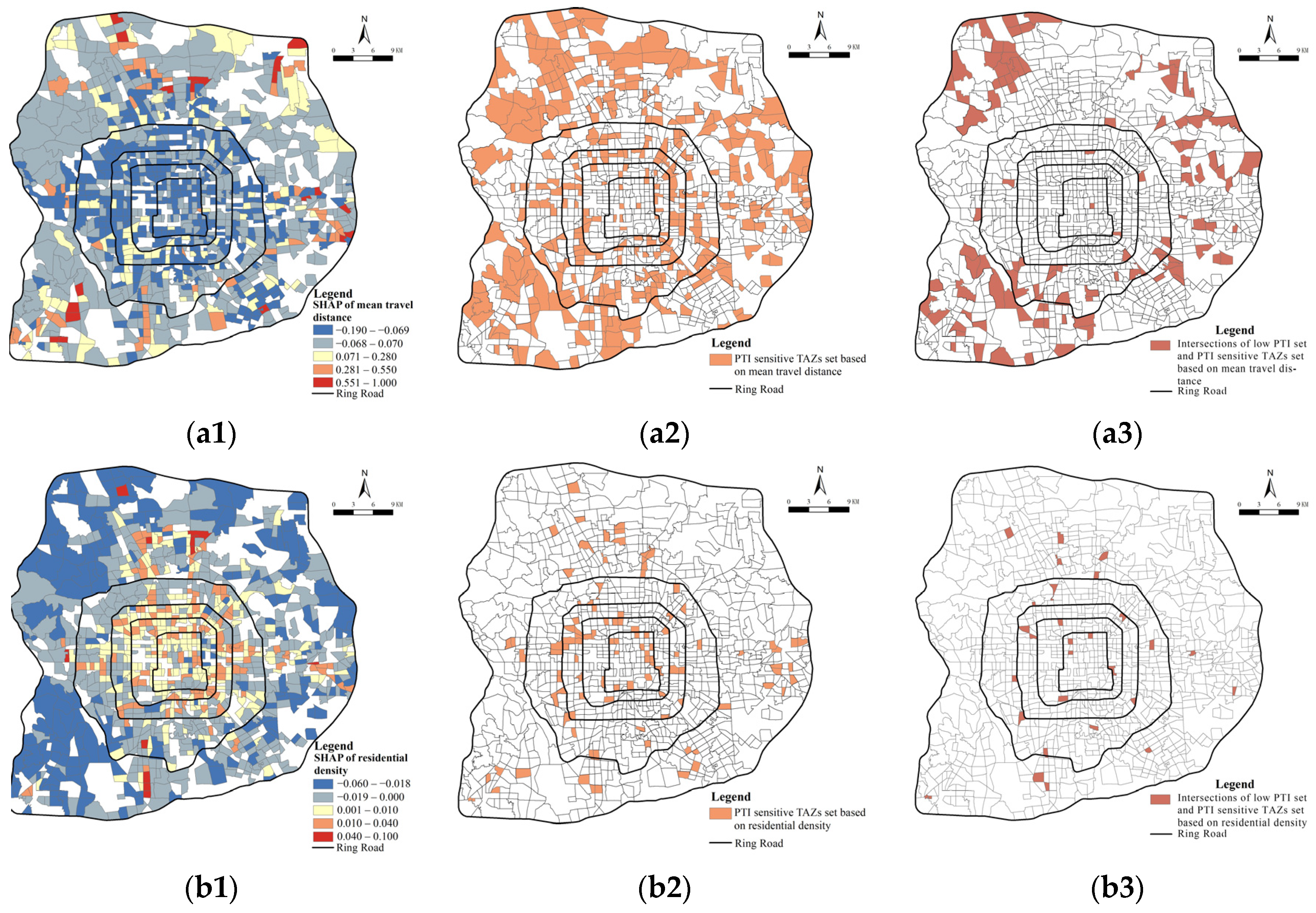
3.4. Spatial Heterogeneity of Land Use Effects on PTI

Figure 6(a1) demonstrates the distribution of SHAP values for mean travel distance. We divided the SHAP values into five categories by using ArcGIS natural breaks classification toolbox. We refer to a TAZ as a “PTI-sensitive TAZ based on mean travel distance” if its mean travel distance falls within the threshold range that substantially influences SHAP value. Figure 6(a2) shows the PTI-sensitive TAZs based on mean travel distance, which are mainly concentrated in the peripheral region. We conducted an intersection analysis of the low-PTI set (Figure 3) and PTI-sensitive TAZs set based on mean travel distance. The TAZs with priority renewals were identified, and the results are shown in Figure 6(a3). These TAZs have a lower PTI and a higher mean travel distance. Although it is shown that increasing the mean travel distance of TAZs within the threshold range can effectively improve PTI in our analysis results, we cannot increase PTI by increasing the mean travel distance. For these TAZs, urban planners and policymakers should, on the one hand, focus on improving public transportation service levels and increasing station accessibility and, on the other hand, analyze other land use factors that significantly affect PTI.
Figure 6(b1) illustrates the distribution of SHAP values for residential density. The TAZs with a high positive influence are distributed in the center and the TAZs with a high negative influence are on the periphery. SHAP values decrease from the center to the periphery. Figure 6(b2) shows the PTI-sensitive TAZs set based on residential density, which are relatively decentralized. We conducted an intersection analysis of the low-PTI set and PTI-sensitive TAZs set based on residential density. The TAZs with priority renewal were identified, and the results are shown in Figure 6(b3). For these TAZs, on the one hand, the residential density can be appropriately increased, and on the other hand, additional station entrances should be established to improve public transportation capacity and increase the density of the public transportation network.
Figure 6(c1) shows the distribution of SHAP values for subway station density. The TAZs with positive influence are mainly distributed in the range between the 2nd Ring Road and the 5th Ring Road, and the TAZs with negative influence are mainly concentrated in the range between the 5th Ring Road and the 6th Ring Road. The SHAP values show decreasing distribution characteristics from the center outward. Compared to the center region, the TAZs located in the northwest have a lower density of subway stations and road networks. However, a large number of long-distance commuters live in the region, and the subway is the main means of commuting during the morning peak hours. Figure 6(c2) shows the PTI-sensitive TAZs based on subway station density, mainly concentrated in the peripheral region. We conducted an intersection analysis of the low-PTI set and PTI-sensitive TAZs set based on subway station density. The TAZs with priority renewal were identified and are mainly concentrated in the southeastern region between the 3rd Ring Road and the 6th Ring Road, as shown in Figure 6(c3). Therefore, opening more subway lines and increasing the number of stations will have a positive effect on these TAZs and improve PTI.
Figure 6(d1) demonstrates the distribution of SHAP values for public services density. The SHAP value as a whole shows decreasing distribution characteristics from the center outward. Figure 6(d2) shows the PTI-sensitive TAZs based on public services density, which are more dispersed. We conducted an intersection analysis of the low-PTI set and PTI-sensitive TAZs set based on public services density. The TAZs with priority renewal were identified, and the results are shown in Figure 6(d3). For these TAZs, it is necessary to analyze the missing types of public service facilities and improve PTI by increasing the density of service facilities.
Figure 6(e1) illustrates the distribution of SHAP values for parking density. The SHAP values indicate that TAZs with high influence are in the periphery, while those with low influence are in the central area. Figure 6(e2) shows the PTI-sensitive TAZs based on parking density. We conducted an intersection analysis of the low-PTI set and PTI-sensitive TAZs set based on parking density. The TAZs with priority renewal were identified, and the results are shown in Figure 6(e3). Corresponding to the distribution of SHAP values, the analysis reveals that the parking density for these TAZs has a negative effect on PTI. This may be due to the fact that residents in TAZs with higher parking density have easy access to parking, and a larger population chooses to use private vehicles to travel. During urban renewal, the parking density in such TAZs should be reduced, and emphasis should be placed on the development of public transportation infrastructure. For the PTI-sensitive TAZs, parking density has a positive effect on SHAP value, possibly because these TAZs have more parking lots for Park and Ride. So, increasing parking density may attract more people to use Park and Ride, and as a result, the PTI of these TAZs will also increase.
Figure 6(f1) demonstrates the distribution of SHAP values for the floor area ratio. Most of the TAZs’ floor area ratios have a positive impact on SHAP. Figure 6(f2) shows the PTI-sensitive TAZs based on floor area ratio. The distribution of these TAZs is more concentrated, mainly within the 5th Ring Road. We conducted an intersection analysis of the low-PTI set and PTI-sensitive TAZs set based on floor area ratio. The TAZs with priority renewal were identified, and the results are shown in Figure 6(f3). They are mainly located between the 3rd Ring Road and 5th Ring Road. For these TAZs, their floor area ratio is between 0.6 and 1.9, and increasing the floor area ratio may increase the bus trip index PTI.
According to the threshold effect results, Wang et al. [61] proposed that for low-vitality rail transit stations, specific built environment variables should be given priority for renewal. However, it is worth noting that correlation is not the same as causation. The results and suggestions in this part are given on the basis of the correlation between explanatory variables and PTI. This correlation may have a certain causal relationship, but the causal relationship still needs more verification. Because urban planning schemes are not like randomized, double-blind trials used in medicine, in order to determine the impact of a certain variable on the results of the experiment, a set of comparison experiments is performed, the variable is changed, and the experimental results are observed.

4. Conclusions and Limitations

This study takes Beijing as an example and uses multi-source big data to compute the land use variables. PTI during the working day’s early peak hours is taken as the dependent variable, and 15 land use and built environment independent variables are selected based on the “7D” dimensions of the built environment. Considering the MAUP, the optimal spatial unit is determined by comparing the goodness of model fitting results of different spatial units. The nonlinear relationship between land use and PTI and the threshold effect was investigated by the XGBoost model. The main conclusions are as follows:
(1)
The results of the study on the impact of land use on PTI are different for different spatial units. A comparison of the goodness of XGBoost of different spatial units shows that the optimal spatial unit to study the impact of land use on PTI in Beijing is TAZ.
(2)
The XGBoost fitting results show that the top four explanatory variables affecting PTI are, in order: mean travel distance, residential density, subway station density, and public services density.
(3)
Some land use and built environment variable have nonlinear effect on PTI and threshold effect results are conducive to propose effective built environment renewal strategies aiming at increasing PTI or public transportation share.
(4)
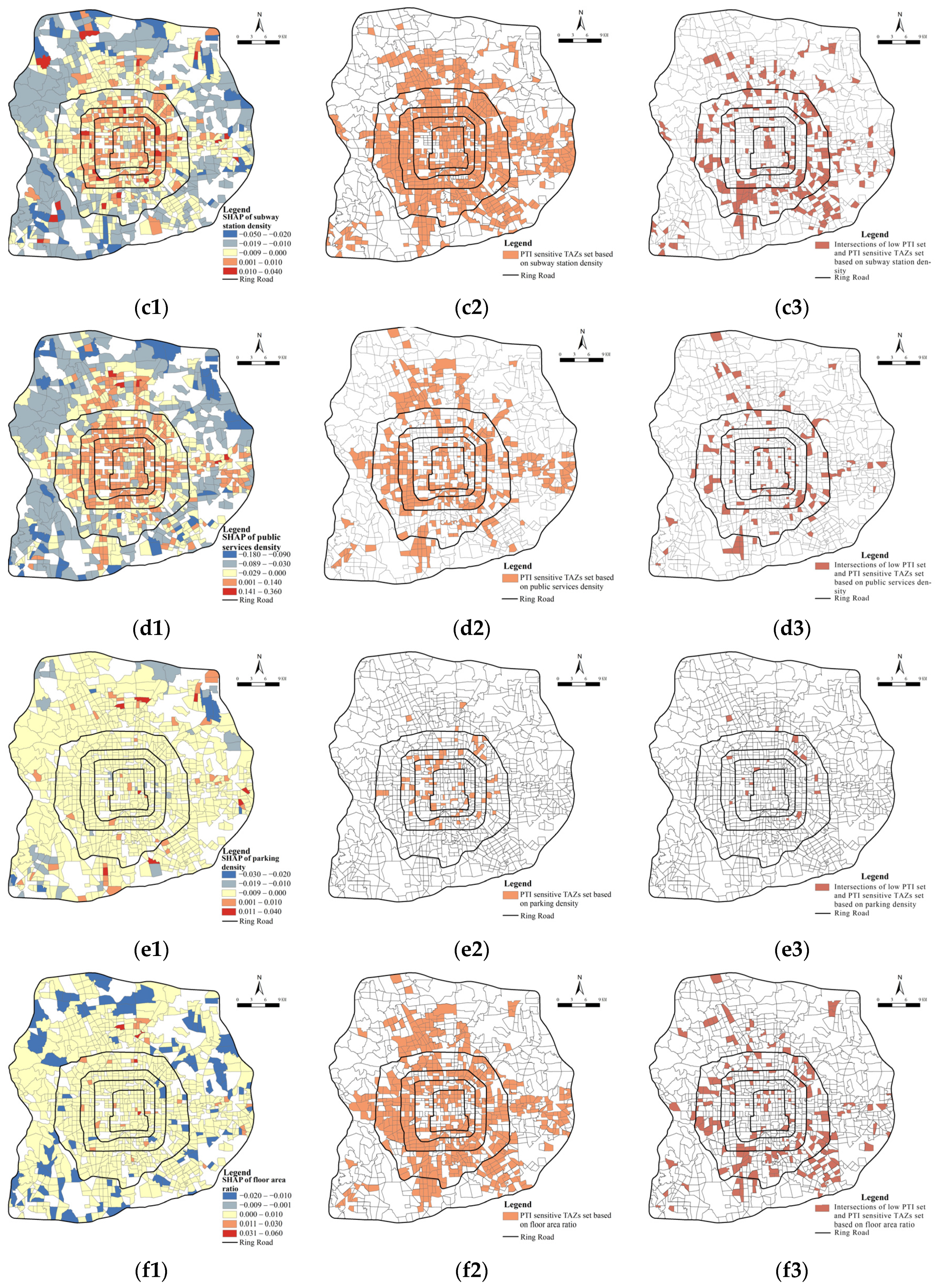
The TAZs with priority renewal were identified according to intersection analysis of the low-PTI set and the PTI-sensitive TAZs based on different land use variables. This has important reference significance for the targeted selection of TAZ for urban built environment renewal.
Although this study fills a gap in research on the effects of partial land use on PTI, there are some limitations: (1) The origin and destination of trips in this research are both bus and subway stations, which is slightly different from the actual origin and destination. (2) This study considers the influence of land use variables on PTI, and does not include other characteristic variables, such as residents’ income and age, and these demographic and economic characteristic variables also have some influence on transport mode choice. (3) Combining other data to identify the OD of other travel modes for accurate public transportation share analysis will be a more meaningful research direction in the future. (4) While machine learning methods can be used to analyze the effect of land use variables on dependent variables, other methods can also be considered for correlation analysis to compare different results. (5) Suggestions for land use and built environment renewal are given on the basis of the correlation between explanatory variables and PTI, which may be different from a real causal relationship, and more verification is needed for causal inference.

Supplementary Materials

The following supporting information can be downloaded at https://www.mdpi.com/article/10.3390/land13081302/s1, Figure S1: Nonlinear relationship and threshold range of other variables on PTI.

Author Contributions

Conceptualization, X.C.; data curation, S.L.; formal analysis, Z.W. and S.L.; investigation, S.L.; methodology, Z.W. and X.C.; project administration, H.L.; resources, Z.W. and H.L.; software, Z.W., S.L. and H.L.; validation, S.L. and H.L.; writing—original draft, Z.W. and S.L.; writing—review and editing, Z.W. and X.C. All authors have read and agreed to the published version of the manuscript.

Funding

Hebei Province Social Science Fund Project, 2019 (No. HB19YS039).

Data Availability Statement

The data used in this study are available from the corresponding author upon reasonable request.

Acknowledgments

The authors would like to express their gratitude to Cui Yidan, a master’s student at Nanjing University, for her valuable suggestions in the process of writing the manuscript.

Conflicts of Interest

The authors declare no conflict of interest.

References

  1. Mraihi, R.; Harizi, R.; Mraihi, T.; Bouzidi, M.T. Urban air pollution and urban daily mobility in large Tunisia’s cities. Renew. Sustain. Energy Rev. 2015, 43, 315–320. [Google Scholar] [CrossRef]
  2. Lee, Z.; Hwang, S.; Kim, J. Optimal Planning of Real-Time Bus Information System for User-Switching Behavior. Electronics 2020, 9, 1903. [Google Scholar] [CrossRef]
  3. Cardozo, O.D.; García-Palomares, J.C.; Gutiérrez, J. Application of geographically weighted regression to the direct forecasting of transit ridership at station-level. Appl. Geogr. 2012, 34, 548–558. [Google Scholar] [CrossRef]
  4. Sun, B.D.; Ermagun, A.; Dan, B. Built environmental impacts on commuting mode choice and distance: Evidence from Shanghai. Transp. Res. Part D Transp. Environ. 2017, 52, 441–453. [Google Scholar] [CrossRef]
  5. Kim, S.; Lee, S. Nonlinear relationships and interaction effects of an urban environment on crime incidence: Application of urban big data and an interpretable machine learning method. Sustain. Cities Soc. 2023, 91, 104419. [Google Scholar] [CrossRef]
  6. Yoshinaga, K.; Onodera, M.; Shirai, K.; Yoshizawa, N.; Yanagawa, H.; Kito, T. Analysis of Stakeholders’ Trust Level in the Nuclear Energy Domain in Japan. J. Nucl. Eng. Radiat. Sci. 2025, 11, 012204. [Google Scholar] [CrossRef]
  7. Saigal, T.; Vaish, A.K.; Rao, N.V.M. Understanding environmentally sustainable Indian travel behaviour: An analysis of 2011 census data. J. Soc. Econ. Dev. 2024, 26, 49–76. [Google Scholar] [CrossRef]
  8. Liu, X.T.; Wu, J.W.; Huang, J.W.; Zhang, J.W.; Chen, B.Y.; Chen, A. Spatial-interaction network analysis of built environmental influence on daily public transport demand. J. Transp. Geogr. 2021, 92, 102991. [Google Scholar] [CrossRef]
  9. An, R.; Wu, Z.H.; Tong, Z.M.; Qin, S.X.; Zhu, Y.; Liu, Y.L. How the built environment promotes public transportation in Wuhan: A multiscale geographically weighted regression analysis. Travel Behav. Soc. 2022, 29, 186–199. [Google Scholar] [CrossRef]
  10. Crotti, D.; Grechi, D.; Maggi, E. Proximity to public transportation and sustainable commuting to college. A case study of an Italian suburban campus. Case Stud. Transp. Policy 2022, 10, 218–226. [Google Scholar] [CrossRef]
  11. Jerrett, M.; Su, J.G.; MacLeod, K.E.; Hanning, C.; Houston, D.; Wolch, J. Safe Routes to Play? Pedestrian and Bicyclist Crashes Near Parks in Los Angeles. Environ. Res. 2016, 151, 742–755. [Google Scholar] [CrossRef]
  12. Nadeem, M.; Matsuyuki, M.; Tanaka, S. Impact of bus rapid transit in shaping transit-oriented development: Evidence from Lahore, Pakistan. J. Asian Archit. Build. Eng. 2023, 22, 3635–3648. [Google Scholar] [CrossRef]
  13. Chakour, V.; Eluru, N. Examining the influence of stop level infrastructure and built environment on bus ridership in Montreal. J. Transp. Geogr. 2016, 51, 205–217. [Google Scholar] [CrossRef]
  14. Goliszek, S. The potential accessibility to workplaces and working-age population by means of public and private car transport in Szczecin. Misc. Geogr. 2022, 26, 31–41. [Google Scholar] [CrossRef]
  15. De Gruyter, C.; Gunn, L.; Kroen, A.; Saghapour, T.; Davern, M.; Higgs, C. Exploring changes in the frequency of public transport use among residents who move to outer suburban greenfield estates. Case Stud. Transp. Policy 2022, 10, 341–353. [Google Scholar] [CrossRef]
  16. Handy, S.L.; Boarnet, M.G.; Ewing, R.; Killingsworth, R.E. How the built environment affects physical activity: Views from urban planning. Am. J. Prev. Med. 2002, 23, 64–73. [Google Scholar] [CrossRef] [PubMed]
  17. Kahn, M.E. A Review of Travel by Design: The Influence of Urban Form on Travel. Reg. Sci. Urban Econ. 2002, 32, 275–277. [Google Scholar] [CrossRef]
  18. Ewing, R.; Cervero, R. Travel and the Built Environment. J. Am. Plan. Assoc. 2010, 76, 265–294. [Google Scholar] [CrossRef]
  19. Larriva, M.T.B.; Büttner, B.; Durán-Rodas, D. Active and healthy ageing: Factors associated with bicycle use and frequency among older adults- A case study in Munich. J. Transp. Health 2024, 35, 101772. [Google Scholar] [CrossRef]
  20. Openshaw, S. A geographical solution to scale and aggregation problems in region-building, partitioning and spatial modelling. Trans. Inst. Br. Geogr. 1977, 2, 459–472. [Google Scholar] [CrossRef]
  21. Lee, S.I.; Lee, M.; Chun, Y.; Griffith, D.A. Uncertainty in the effects of the modifiable areal unit problem under different levels of spatial autocorrelation: A simulation study. Int. J. Geogr. Inf. Sci. 2019, 33, 1135–1154. [Google Scholar] [CrossRef]
  22. Gao, F.; Li, S.Y.; Tan, Z.Z.; Wu, Z.F.; Zhang, X.M.; Huang, G.P.; Huang, Z.W. Understanding the modifiable areal unit problem in dockless bike sharing usage and exploring the interactive effects of built environment factors. Int. J. Geogr. Inf. Sci. 2021, 35, 1905–1925. [Google Scholar] [CrossRef]
  23. Mills, O.; Shackleton, N.; Colbert, J.; Zhao, J.F.; Norman, P.; Exeter, D.J. Inter-relationships between geographical scale, socio-economic data suppression and population homogeneity. Appl. Spat. Anal. Policy 2022, 15, 1075–1091. [Google Scholar] [CrossRef]
  24. Altan, M.F.; Ayozen, Y.E. The Effect of the Size of Traffic Analysis Zones on the Quality of Transport Demand Forecasts and Travel Assignments. Period. Polytech.Civ. Eng. 2018, 62, 971–979. [Google Scholar] [CrossRef]
  25. Sun, G.D.; Chang, B.F.; Zhu, L.; Wu, H.; Zheng, K.; Liang, R.H. TZVis: Visual analysis of bicycle data for traffic zone division. J. Vis. 2019, 22, 1193–1208. [Google Scholar] [CrossRef]
  26. Thomsen, N. Implementing a Ride-sharing Algorithm in the German National Transport Model (DEMO). Transp. Res. Rec. 2023, 2677, 1–10. [Google Scholar] [CrossRef]
  27. Lee, J.; Kang, T.W.; Choi, Y.S.; Jung, J.W. Clearance-Based Performance-Efficient Path Planning Using Generalized Voronoi Diagram. Int. J. Fuzzy Log. Intell. Syst. 2023, 23, 259–269. [Google Scholar] [CrossRef]
  28. Breitkreutz, D.; Lee, I. Investigation into Alternative Representations for Intelligent Geoinformation Systems in Data-rich Environments. J. Softw. 2009, 4, 777–784. [Google Scholar] [CrossRef]
  29. Ketterer, C.; Gangwisch, M.; Fröhlich, D.; Matzarakis, A. Comparison of selected approaches for urban roughness determination based on voronoi cells. Int. J. Biometeorol. 2017, 61, 189–198. [Google Scholar] [CrossRef]
  30. Ordoñez, D.M.T.; Batac, R.C. Cascade events in geographical space. Int. J. Mod. Phys. C 2022, 33, 2250050. [Google Scholar] [CrossRef]
  31. Nguyen, Q.C.; Tasdizen, T.; Alirezaei, M.; Mane, H.; Yue, X.H.; Merchant, J.S.; Yu, W.J.; Drew, L.; Li, D.P.; Nguyen, T.T. Neighborhood built environment, obesity, and diabetes: A Utah siblings study. SSM-Popul. Health 2024, 26, 101670. [Google Scholar] [CrossRef]
  32. Nguyen, Q.C.; Sajjadi, M.; McCullough, M.; Pham, M.; Nguyen, T.T.; Yu, W.J.; Meng, H.W.; Wen, M.; Li, F.F.; Smith, K.R.; et al. Neighbourhood looking glass: 360° automated characterisation of the built environment for neighbourhood effects research. J. Epidemiol. Community Health 2018, 72, 260–266. [Google Scholar] [CrossRef]
  33. Mazumdar, S.; Jaques, K.; Conaty, S.; De Leeuw, E.; Gudes, O.; Lee, J.W.; Prior, J.; Bin, J.; Harris, P. Hotspots of change in use of public transport to work: A geospatial mixed method study. J. Transp. Health 2023, 31, 101650. [Google Scholar] [CrossRef]
  34. Pei, T.; Sobolevsky, S.; Ratti, C.; Shaw, S.L.; Li, T.; Zhou, C.H. A new insight into land use classification based on aggregated mobile phone data. Int. J. Geogr. Inf. Sci. 2014, 28, 1988–2007. [Google Scholar] [CrossRef]
  35. Wali, B.; Santi, P.; Ratti, C. A joint demand modeling framework for ride-sourcing and dynamic ridesharing services: A geo-additive Markov random field based heterogeneous copula framework. Transportation 2023, 50, 1809–1845. [Google Scholar] [CrossRef]
  36. Correia, G.H.D.; Silva, J.D.E.; Viegas, J.M. Using latent attitudinal variables estimated through a structural equations model for understanding carpooling propensity. Transp. Plan. Technol. 2013, 36, 499–519. [Google Scholar] [CrossRef]
  37. Singh, Y.R.; Shah, D.B.; Kulkarni, M.; Patel, S.R.; Maheshwari, D.G.; Shah, J.S.; Shah, S. Current trends in chromatographic prediction using artificial intelligence and machine learning. Anal. Methods 2023, 15, 2785–2797. [Google Scholar] [CrossRef] [PubMed]
  38. Cervero, R.; Kockelman, K. Travel demand and the 3Ds: Density, diversity, and design. Transp. Res. Part D Transp. Environ. 1997, 2, 199–219. [Google Scholar] [CrossRef]
  39. Uddin, M.; Anowar, S.; Eluru, N. Modeling freight mode choice using machine learning classifiers: A comparative study using Commodity Flow Survey (CFS) data. Transp. Plan. Technol. 2021, 44, 543–559. [Google Scholar] [CrossRef]
  40. Fakhri, D.; Khodayari, A.; Mahmoodzadeh, A.; Hosseini, M.; Ibrahim, H.H.; Mohammed, A.H. Prediction of Mixed-mode I and II effective fracture toughness of several types of concrete using the extreme gradient boosting method and metaheuristic optimization algorithms. Eng. Fract. Mech. 2022, 276, 108916. [Google Scholar] [CrossRef]
  41. Metzler, A.B.; Nathvani, R.; Sharmanska, V.; Bai, W.; Muller, E.; Moulds, S.; Agyei-Asabere, C.; Adjei-Boadi, D.; Kyere-Gyeabour, E.; Tetteh, J.D.; et al. Phenotyping urban built and natural environments with high-resolution satellite images and unsupervised deep learning. Sci. Total Environ. 2023, 893, 164794. [Google Scholar] [CrossRef]
  42. Sibindi, R.; Mwangi, R.W.; Waititu, A.G. A boosting ensemble learning based hybrid light gradient boosting machine and extreme gradient boosting model for predicting house prices. Eng. Rep. 2023, 5, e12599. [Google Scholar] [CrossRef]
  43. Elorza, M.; Castellano, E.; Segura, S. Prediction of customer demand for perishable products in retail inventory management, using the hybrid prophet-XGBoost model during the post-COVID-19 period. Appl. Econ. Lett. 2024, 1–7. [Google Scholar] [CrossRef]
  44. Fatty, A.; Li, A.J.; Qian, Z.G. An interpretable evolutionary extreme gradient boosting algorithm for rock slope stability assessment. Multimed. Tools Appl. 2023, 83, 46851–46874. [Google Scholar] [CrossRef]
  45. Rabby, Y.W.; Hossain, M.B.; Abedin, J. Landslide susceptibility mapping in three Upazilas of Rangamati hill district Bangladesh: Application and comparison of GIS-based machine learning methods. Geocarto Int. 2022, 37, 3371–3396. [Google Scholar] [CrossRef]
  46. Indhumathi, K.; Kumar, K.S. Efficient Prediction of Seasonal Infectious Diseases Using Hybrid Machine Learning Algorithms with Feature Selection Techniques. Int. J. Artif. Intell. Tools 2023, 32, 2350044. [Google Scholar] [CrossRef]
  47. Garcia-Retuerta, D.; Chamoso, P.; Hernández, G.; Guzmán, A.S.; Yigitcanlar, T.; Corchado, J.M. An Efficient Management Platform for Developing Smart Cities: Solution for Real-Time and Future Crowd Detection. Electronics 2021, 10, 765. [Google Scholar] [CrossRef]
  48. dos Santos, R.D., Jr.; Coelho, J.V.V.; Cacho, N.A.A.; de Araujo, D.S.A. A criminal macrocause classification model: An enhancement for violent crime analysis considering an unbalanced dataset. Expert Syst. Appl. 2024, 238, 121702. [Google Scholar] [CrossRef]
  49. Liu, J.X.; Xiao, L.Z.; Zhou, J.P.; Yang, L.C. Non-linear relationships between the built environment and walking to school: Applying extreme gradient boosting method. Prog. Geogr. 2022, 41, 251–263. [Google Scholar] [CrossRef]
  50. Shaik, R.U.; Unni, A.; Zeng, W.P. Quantum Based Pseudo-Labelling for Hyperspectral Imagery: A Simple and Efficient Semi-Supervised Learning Method for Machine Learning Classifiers. Remote Sens. 2022, 14, 5774. [Google Scholar] [CrossRef]
  51. Huang, B.; Wu, B.; Barry, M. Geographically and temporally weighted regression for modeling spatio-temporal variation in house prices. Int. J. Geogr. Inf. Sci. 2010, 24, 383–401. [Google Scholar] [CrossRef]
  52. Frank, L.D.; Pivo, G. Impacts of mixed use and density on utilization of three modes of travel: Single-occupant vehicle, transit, and walking. Transp. Res. Record 1994, 14, 44–52. [Google Scholar]
  53. Tao, T.; Cao, J. Exploring nonlinear and collective influences of regional and local built environment characteristics on travel distances by mode. J. Transp. Geogr. 2023, 109, 103599. [Google Scholar] [CrossRef]
  54. Lundberg, S.M.; Erion, G.G.; Su-In, L. Consistent Individualized Feature Attribution for Tree Ensembles. arXiv 2018, arXiv:1802.03888. [Google Scholar]
  55. Shannon, C.E.; Weaver, W. A Mathematical Theory of Communication. Philos. Rev. 1949, 5, 3–55. [Google Scholar]
  56. Wang, Z.B.; Wang, S.C.; Lian, H.T. A route-planning method for long-distance commuter express bus service based on OD estimation from mobile phone location data: The case of the Changping Corridor in Beijing. Public Transp. 2021, 13, 101–125. [Google Scholar] [CrossRef]
  57. Ji, S.; Wang, X.; Lyu, T.; Liu, X.; Wang, Y.; Heinen, E.; Sun, Z. Understanding cycling distance according to the prediction of the XGBoost and the interpretation of SHAP: A non-linear and interaction effect analysis. J. Transp. Geogr. 2022, 103, 103414. [Google Scholar] [CrossRef]
  58. Liu, X.; Chen, X.; Tian, M.; De Vos, J. Effects of buffer size on associations between the built environment and metro ridership: A machine learning-based sensitive analysis. J. Transp. Geogr. 2023, 113, 103730. [Google Scholar] [CrossRef]
  59. Han, H.R.; Yang, C.F.; Wang, E.R.; Song, J.P.; Zhang, M. Evolution of jobs-housing spatial relationship in Beijing Metropolitan Area: A job accessibility perspective. Chin. Geogr. Sci. 2015, 25, 375–388. [Google Scholar] [CrossRef]
  60. Currie, G.; Delbosc, A. Understanding bus rapid transit route ridership drivers: An empirical study of Australian BRT systems. Transp. Policy 2011, 18, 755–764. [Google Scholar] [CrossRef]
  61. Wang, Z.; Li, S.; Zhang, Y.; Wang, X.; Liu, S.; Liu, D. Built Environment Renewal Strategies Aimed at Improving Metro Station Vitality via the Interpretable Machine Learning Method: A Case Study of Beijing. Sustainability 2024, 16, 1178. [Google Scholar] [CrossRef]
Figure 1. Study area. (a) Location of study area in Beijing; (b) the spatial distribution of subway stations; (c) the spatial distribution of bus stations.
Land 13 01302 g001
Figure 2. The schematic diagram of spatial unit division.
Land 13 01302 g002
Figure 3. Spatial distribution of PTI.
Land 13 01302 g003
Figure 4. Global impact of explanatory variables on PTI.
Land 13 01302 g004
Figure 5. Nonlinear relationships and threshold ranges of land use variables on PTI. (a) Mean travel distance; (b) residential density; (c) subway station density; (d) public services density; (e) parking density; (f) floor area ratio.
Land 13 01302 g005aLand 13 01302 g005b
Figure 6. The spatial distribution of SHAP values for land use variables, nonlinear threshold effects, and the intersection of nonlinear threshold and PTI. (a1) SHAP values for mean travel distance; (a2) PTI-sensitive TAZs based on mean travel distance. (a3) Intersection of low PTI set and sensitive TAZs based on mean travel distance and PTI; (b1) SHAP values for residential density; (b2) PTI-sensitive TAZs based on residential density; (b3) intersection of the low-PTI set and sensitive TAZs based on residential density; (c1) SHAP values for subway station density; (c2) PTI-sensitive TAZs based on subway station density; (c3) intersection of the low-PTI set and sensitive TAZs based on subway station density; (d1) SHAP values for public services density; (d2) PTI sensitive TAZs based on public services density; (d3) intersection of the low-PTI set and sensitive TAZs based on public services density; (e1) SHAP of parking density; (e2) PTI-sensitive TAZs based on parking density; (e3) intersection of the low PTI-set and sensitive TAZs based on parking density; (f1) SHAP values for floor area ratio; (f2) PTI-sensitive TAZs based on floor area ratio; (f3) intersection of low-PTI set and sensitive TAZs based on floor area ratio.
Land 13 01302 g006aLand 13 01302 g006b
Table 1. Public transportation trip record data.
Traveler Number Starting Station Longitude of Origin StationLatitude of Origin StationBoarding TimeDestination Station Longitude of Destination StationLatitude of Destination StationAlighting TimeTravel Distance (m)
1Heping Men116.384239.900113 October 2020 9:00Huilong Guan116.336140.070813 October 2020 10:0522,946.03
2Jianguo Men116.435839.908513 October 2020 9:01Jishuitan116.373139.9486513 October 2020 9:409818.436
3Weigong Village116.323839.952913 October 2020 9:05Baishiqiao Nan116.325539.9362613 October 2020 9:251986.12
4Zhongguan Village116.316539.9839913 October 2020 9:08Tiantong Yuan116.412840.0752213 October 2020 10:2018,355.52
Table 2. Land use and built environment variables.
“7D” DimensionsVariablesMain CategoryDescriptionUnitMeanStd. Dev.Data Sources
DensityBuilding densityLand use and built environmentTotal building base area divided by the spatial unit’s areakm/km20.170.09Open street map
(https://lbs.amap.com/, accessed on 10 July 2022)
Commercial densityLand useThe number of commercial facilities divided by the spatial unit’s areaquantity/km299.85106.87
Public services densityLand useThe number of public service facilities divided by the spatial unit’s areaquantity/km257.3764.89
Office densityLand useThe number of office facilities divided by the spatial unit’s areaquantity/km2120.76159.96
Residential densityLand use and built environmentThe number of residents divided by the spatial unit’s areaperson/km219,357.1118,332.60Cell phone data [56]
DiversityDiversity index of mixed land useLand use and built environmentDiversity index H = P i ln P i , P i is the ratio of the number of the ith class POIs to the number of all POIs. 0.960.13Amap API
(https://lbs.amap.com/, accessed on 10 July 2022)
DesignRoad network density Land use and built environmentLength of road divided by the spatial unit’s areakm/km24.953.08Open street map
(https://www.openstreetmap.org/, accessed on 10 July 2022)
Floor area ratioLand use and built environmentThe total construction area divided by the spatial unit’s area 1.000.72
Destination accessibilityMean travel distanceBuilt environmentThe average Manhattan distance of all public transportation trips whose origin locations are within a TAZm10,364.384329.88Processed transit trip record data based on IC card payments for public transportation (courtesy of Beijing Traffic Management)
Distance to transitPublic transportation network densityLand use and built environmentLength of public transport lines divided by the spatial unit’s areakm/km228.8425.74Open street map
(https://www.openstreetmap.org/, accessed on 10 July 2022)
Bus station densityBuilt environmentThe number of bus stations divided by the spatial unit’s areaquantity/km234.0831.13
Subway station densityBuilt environmentThe number of subway stations divided by the spatial unit’s areaquantity/km20.980.72
Vertical distance from the bus stop to the nearest primary road or trunk roadBuilt environmentThe mean value of vertical distance from the bus stop to the nearest primary road or trunk roadkm2.203.09
Demand managementParking densityLand use and built environmentThe number of parking lots divided by the spatial unit’s areaquantity/km232.5736.27Amap API (https://lbs.amap.com/, accessed on 10 July 2022)
DemographicsPopulation densityBuilt environmentThe population count divided by the spatial unit’s areapersons/km28856.575080.17Data from WorldPop (https://hub.worldpop.org/geodata/summary?id=24926, accessed on 10 July 2022)
Table 3. The MAE, MSE, MAPE, RMSE, and R2 comparison results of the testing dataset of XGBoost for different spatial units.
Spatial UnitAverge Spatial Unit Area (m2)R2MAEMSERMSEMAPE
200 m × 200 m40,0000.271.1713.323.656.94
300 m × 300 m90,0000.320.150.230.485.02
400 m × 400 m160,0000.070.401.461.216.05
500 m × 500 m250,0000.010.320.740.866.99
600 m × 600 m360,0000.180.280.890.946.43
700 m × 700 m490,0000.330.210.350.594.03
800 m × 800 m640,0000.230.170.170.414.70
900 m × 900 m810,0000.010.180.130.366.26
1000 m × 1000 m1,000,0000.210.180.280.533.80
1100 m × 1100 m1,210,0000.320.130.080.293.62
1200 m × 1200 m1,440,0000.060.130.060.256.26
1300 m × 1300 m1,690,0000.230.120.060.255.25
1400 m × 1400 m1,960,0000.220.110.040.205.67
1500 m × 1500 m2,250,0000.120.110.040.205.41
1600 m × 1600 m2,560,0000.160.090.020.135.76
1700 m × 1700 m2,890,0000.230.110.040.214.30
1800 m × 1800 m3,240,0000.030.120.040.204.04
1900 m × 1900 m3,610,0000.300.100.040.206.04
2000 m × 2000 m4,000,0000.340.100.030.164.26
TAZs1,721,7350.620.090.020.133.48
neighborhood11,994,5170.000.230.210.466.19
Disclaimer/Publisher’s Note: The statements, opinions and data contained in all publications are solely those of the individual author(s) and contributor(s) and not of MDPI and/or the editor(s). MDPI and/or the editor(s) disclaim responsibility for any injury to people or property resulting from any ideas, methods, instructions or products referred to in the content.

