Abstract
(1) Background: The use of multiscale prediction or the optimal scaling of predictors can enhance soil maps by applying pixel size in digital soil mapping (DSM). (2) Methods: A total of 200, 50, and 129 surface soil samples (0–30 cm) were collected by the CLHS method in three different areas, namely, the Marvdasht, Bandamir, and Lapuee plains in southwest Iran. Then, four soil properties—soil organic matter (SOM), bulk density (BD), soil shear strength (SS), and mean weighted diameter (MWD)—were measured at each sampling point as representative attributes of soil physical and chemical quality. This study examined different-scale scenarios ranging from resampling the original 30 m digital elevation model and remote sensing indices to various pixel sizes, including 60 × 60, 90 × 90, 120 × 120, and up to 2100 × 2100 m. (3) Results: After evaluating 22 environmental covariates, 11 of them were identified as the most suitable candidates for predicting soil properties based on recursive feature elimination (RFE) and expert opinion methods. Furthermore, among different pixel size scenarios for SOM, BD, SS, and MWD, the highest accuracy was achieved at 1200 × 1200 m (R2 = 0.35), 180 × 180 m (R2 = 0.67), 1200 × 1200 m (R2 = 0.42), and 2100 × 2100 m (R2 = 0.34), respectively, in Marvdasht plain. (4) Conclusions: Adjusting the pixel size improves the capture of soil property variability, enhancing mapping precision and supporting effective decision making for crop management, irrigation, and land use planning.
1. Introduction
The physio-chemical properties of soil play a crucial role and exert a direct influence on the productivity of agricultural land [1]. Consequently, the effective management of soil properties is of utmost importance for the sustainable and healthy maintenance of agricultural yields [2]. Therefore, the prediction and mapping of soil properties are essential procedures for achieving this sustainability [3].
In most regions of Iran, the measurement of soil physio-chemical properties relies on labor-intensive and costly procedures. Hence, numerous scientists have dedicated substantial efforts to developing dependable and cost-effective methods for generating improved and current mapping of soil physio-chemical properties [4,5]. In this regard, the integration of remote sensing (RS) data, gamma-ray measurements, and topographic features with digital soil mapping (DSM) was essential in identifying unique patterns. This combination significantly contributed to revealing and understanding trends relevant to soil processes and management practices [6]. Similarly to laboratory measurements, RS predictions can be used as “s” and “o” factors in the SCORPAN model, i.e., clay mineral and vegetation indices [7]. Also, RS plays a pivotal role in enhancing DSM by extending existing soil survey data sets. It provides valuable data that can be utilized in several ways. Firstly, RS aids in segmenting the landscape into more homogeneous soil–landscape units, allowing for more accurate assessments of soil composition through targeted sampling methods. Secondly, the data derived from RS can be analyzed using both physically and empirically based techniques to accurately derive soil properties [8]. Importantly, RS significantly enhances the ability to map inaccessible areas, minimizing the reliance on extensive, time-consuming, and costly field surveys [9,10].
DSM, coupled with spatial soil data presented as cartographic representations, is indispensable for the comprehensive evaluations of soil quality, the prediction of soil properties, the implementation of sustainable land use strategies, and the conduct of precision farming research [11,12].
The influence of land-surface derivatives on predicting soil properties within the framework of DSM is scale-dependent. Environmental variables play a significant role in DSM and have varying effects across different scales of the landscape [13]. The use of multiscale predictors or the optimal scaling of predictors can enhance soil maps by applying pixel size in DSM [14]. Considering the importance of scale in influencing the accuracy of spatial prediction of soil properties [15], recent pedometric studies have primarily focused on DSM studies, particularly in terms of predicting the quality or comparing the performance of algorithms [14]. However, there has been less emphasis on in-depth investigations into this specific area of scientific soil mapping. Only a few studies, such as [15,16], have delved into the depth of this aspect, with a focus on soil classes or taxa. In this regard, Sena [17] utilized digital elevation model (DEM) data with different pixel sizes (2, 12.5, and 30 m) to predict soil classes. The findings revealed that terrain attributes obtained from the 30 m DEM exhibited a notably high level of accuracy in predicting soil classes. In a separate investigation, Maleki [18] observed improved precision in soil class prediction when using terrain attributes derived from an unmanned aerial vehicle DEM with a spatial resolution of 30 meters, compared to a standard 5-meter-resolution DEM. Moreover, these studies predominantly concentrated on soil classes rather than exploring the need for further parameterization and knowledge discovery in this field. Therefore, there is a significant need for more extensive research and exploration of soil properties within the realm of DSM to enhance our understanding and improve the predictive capabilities in this domain. Although recent studies by researchers have focused on certain soil properties such as Dornik [19] in Romania, these studies have solely considered the impact of the scale of terrain derivatives. Additionally, they have only considered limited ranges of pixel sizes and have not evaluated higher comparative ranges, for example, those larger scales (i.e., more than 1000 m). Furthermore, these studies have been conducted solely in a specific study area and have not addressed the extrapolation of their findings [20].
Globally, the availability of soil data for DSM models varies significantly. Some regions have well-developed soil databases, while others have low sampling density [21]. When attempting to transfer a DSM model fitted from an area with a well-developed soil database to areas with a low sampling density, challenges arise [22,23]. This is due to the fact that different regions of the world seldom have the same soil-forming factors. As a result, mapping soil in areas with a low sampling density based on a DSM model from a different region is a difficult task [3]. The ability to transfer a spatial model from one region (reference area) to another is given (receptor area) when there is significant similarity and agreement between the indicative environmental covariates. This is commonly referred to as spatial homogeneity, and the spatial models can be transferred from the reference area to the receptor area [11].
The Homosoil theory proves to be a valuable hypothesis for statistical analysis and modeling, facilitating the transfer of soil properties from one area to another using appropriate statistical models. This theory proves to be particularly beneficial in scenarios where there is a lack of sufficient data in the target region. It helps researchers to refine their models by using available data from analogous areas [21]. In previous research by Khosravani et al. [3], the Homosoil theory was utilized to extrapolate a digital map of four crucial soil fertility properties, including soil organic carbon, total nitrogen, available phosphorus, and exchangeable potassium. This was achieved by employing three machine learning algorithms (MLAs) and a pool of environmental covariates, with a basic pixel size of 30m. However, the researchers did not consider the effect scale of environmental covariates in their analysis, which presents an area for further investigation. In a similar vein, Hateffard et al. [11] examined the extrapolation effects of a random forest ML model in predicting topsoil properties in four African countries. Their findings revealed that despite acceptable cross-validation results for the trained models, the extrapolation results were unsatisfactory, underscoring the risks associated with extrapolation in geographic and feature space. The study underscored the constraints of specific measures and the necessity for additional research to tackle the impacts of extrapolation in DSM models.
The selected study regions are known for their intensive agricultural productivity, growing various annual crops throughout the year [3]. However, there is a lack of information regarding the spatial variability of soil physicochemical properties influenced by environmental covariates at different scales. The proposed research shows exceptional promise as it explores the underexplored aspects of scale and extrapolation within spatial models in the context of DSM. By relying on previous research, the current study is based on the hypothesis that integrating scale considerations and extrapolation techniques in spatial models for DSM will result in enhanced predictive accuracy and a deeper understanding of soil property variability across various spatial scales. To address this hypothesis, this study aims to achieve the following objectives: (i) identify the optimal scale for spatial variations of selected soil properties (i.e., soil organic matter, bulk density, soil shear strength, and mean weighted diameter), (ii) apply a theoretical framework for knowledge transfer between reference and receptor areas, (iii) identify influential environmental factors and their spatial scales for predicting soil properties, and (iv) evaluate the predictive capability of the XGBoost model across different-scale scenarios and extrapolate a soil spatial model from the Marvdasht plain as a reference area to the Bandamir and Lapuee plains as receptor areas in southwest Iran.
2. Materials and Methods
2.1. Description of Study Sites
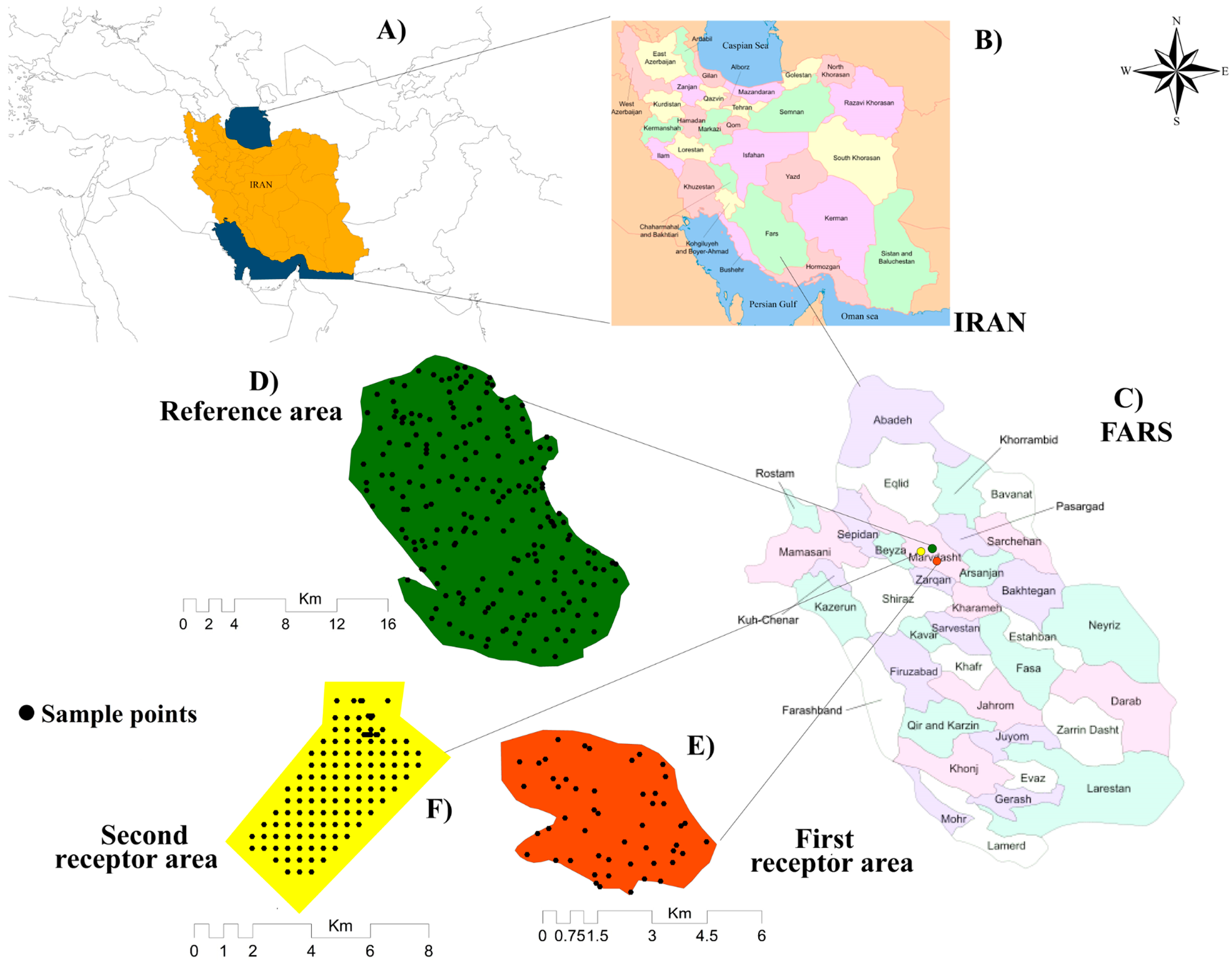
This study was conducted in agricultural zones within the Fars province in southwest Iran, covering the Marvdasht plain as the reference area, and the Bandamir and Lapuee plains as the receptor areas, as shown in Figure 1.

Figure 1.
Geographic Locations of study areas. (A) The country of Iran highlighted on a world map; (B) Fars province indicated by an arrow in a distinctive light green color among other provinces; (C) detailed map of Fars province divisions and the specific locations of the studied areas; (D) the Marvdasht plain depicted as a vivid green polygon area, with clearly marked sample points; (E) the Bandamir plain highlighted by a bold red polygon, along with the precise locations of the sampling points; (F) the Lapuee plain represented by a striking yellow polygon, with corresponding sampling points.
2.1.1. Reference Area
The Marvdasht plain spans 48,963 ha, with specific geographical coordinates 52°41′35.82″ to 52°57′1.07″ E and from latitude 30°2′14.72″ to 29°48′35.02″ N (Figure 1D). The mean annual temperature and precipitation are 17.57 °C and 287.63 mm, and the soil moisture and temperature regimes are xeric and thermic, respectively, according to the nearest meteorological station. The area features specific soil characteristics and is classified under the order taxonomic levels of Entisols and Inceptisols. The main parent materials found in this area consist of carbon-rich soils, alluvial colluvial deposits, and other materials associated with the Quaternary period. It is characterized by three main typical landscapes, including piedmont, alluvial plain, and mountain, with the reference area being relatively flat and having low physiography complexity. The primary land use in the Marvdasht plain predominantly consists of irrigated crop cultivation, including crops such as winter wheat, canola, barley, and alfalfa. Additionally, dry farming practices are employed in some parts of the area, and there are also sections designated as pastures. The Marvdasht plain was chosen as the reference area for our study due to its substantial size and extensive coverage of soil observations. Its large expanse and dense soil observation network made it an ideal candidate for serving as the reference area in our analysis.
2.1.2. First Receptor Area
The Bandamir plain, as the first receptor area covering an area of 7000 hectares, is located approximately 7 km south of the Marvdasht plain (Figure 1E). Its geographical coordinates range from a longitude of 52°49′56.76″ to 52°55′50.56” E and from a latitude of 29°44′32.68″ to 29°39′52.24″ N. In terms of climatical data, the mean annual temperature and precipitation are 17.57 °C and 287.63 mm, and the soil moisture and temperature regimes are xeric and thermic, respectively. The soil classification in the Bandamir plain shares the same taxonomic orders as the reference area. The Bandamir plain is characterized by three primary landscapes, namely piedmont, alluvial plain, and hilland. Similarly, to the reference area, the Bandamir plain is relatively flat, with an elevation ranging from 1570 to 1600 m.s.l. Additionally, more than 80% of the land in the Bandamir plain is located on slopes that are lower than 5%. The main land uses of the Bandamir plain are the cultivation of irrigation crops, dry farming, and in some parts, pastures.
2.1.3. Second Receptor Area
The Lapuee plain, the second receptor area, covers an area of 5000 hectares and is situated approximately 10 kilometers west of the reference area. It spans between 29°78′ to 29°88′ E and 52°68′ to 52°71′ N. In terms of climatic conditions, the Lapuee plain experiences a mean annual temperature of 17 °C and receives an average annual precipitation of 446 mm. The soil moisture and temperature regimes are xeric and thermic, respectively [24]. The parent materials found in the soils of this area consist of lime, shale, alluvial/colluvial, and deposits which are associated with the Quaternary period. The soil classification in the study area primarily falls under the two main orders of Entisols and Inceptisols [25]. The region is characterized by three main landscape types, namely plain, piedmont, and hilland from south to north. The Lapuee plain itself is predominantly flat, with an elevation ranging from 1591 to 1900 m.s.l. Similarly to the other areas, the Lapuee plain is primarily composed of flat terrain, with plain and piedmont landscapes covering over 85% of the total area, and these areas are located on slopes that are lower than 5% (Figure 1F). The dominant land uses of this area are irrigated land, dry farming, and pastures from plain to hilland landscapes.
2.2. Soil Sampling and Laboratory Analysis
A survey campaign was thus conducted, and a total of 200, 50, and 129 locations were collected from the topsoil (0–30 cm) for the reference (Marvdasht), the first (Bandamir), and the second (Lapuee plain) receptor areas, respectively. The Latin hypercube sampling (CLHS) method, as one of the most common and accurate modern soil sampling techniques, was used in this study to determine the locations of soil sampling points [26]. After identifying the relevant environmental covariates, the calibration process for the CLHS repetition against the objective function was established through 12,000 iterations. This served as the basis for selecting the final distribution pattern generated by the CLHS method. The environmental covariates included the Wetness Index, Wind Effect, Perpendicular Vegetation Index, and Valley depth, which were determined using expert opinion methods. Prior to the laboratory measurements, the soil samples were air-dried and passed through a 2 mm sieve. Soil organic matter (SOM) was measured via the wet combustion method [27], bulk density (BD) was measured via the cylinder method, and mean weighted diameter (MWD) values were calculated based on standard procedures [28] in the laboratory. The shear strength (SS) content was determined using the Torvin resistance tester. It should be noted that the SS content at each point was determined from the average of three measurements taken at equal intervals along the circumference of a circle with a diameter of approximately 0.5 m.
2.3. Auxiliary Variables and Scales Scenarios
2.3.1. Auxiliary Variables
Two distinct sets of environmental variables, specifically Sentinel-2 and Landsat 8 remote sensing (RS) images along with terrain attributes derived from a digital elevation model (DEM), were gathered for serving as readily accessible proxies of soil-forming factors to predict desired soil properties (Table 1). These environmental covariates were standardized to the WGS84 UTM Zone 39N projection in R statistical software (4.2.1). The time series of remote sensing (RS) images used in this study were collected from May to August 2021 via the Google Earth Engine platform. All images selected for analysis had less than 10% cloud cover, ensuring high-quality data for accurate interpretation of the landscape changes during this period. To handle the large amount of RS data, we combined them using principal component analysis. Additionally, combining RS data has shown improved precision of prediction [29].

Table 1.
The environmental covariates utilized in this research.
2.3.2. Scales Scenarios
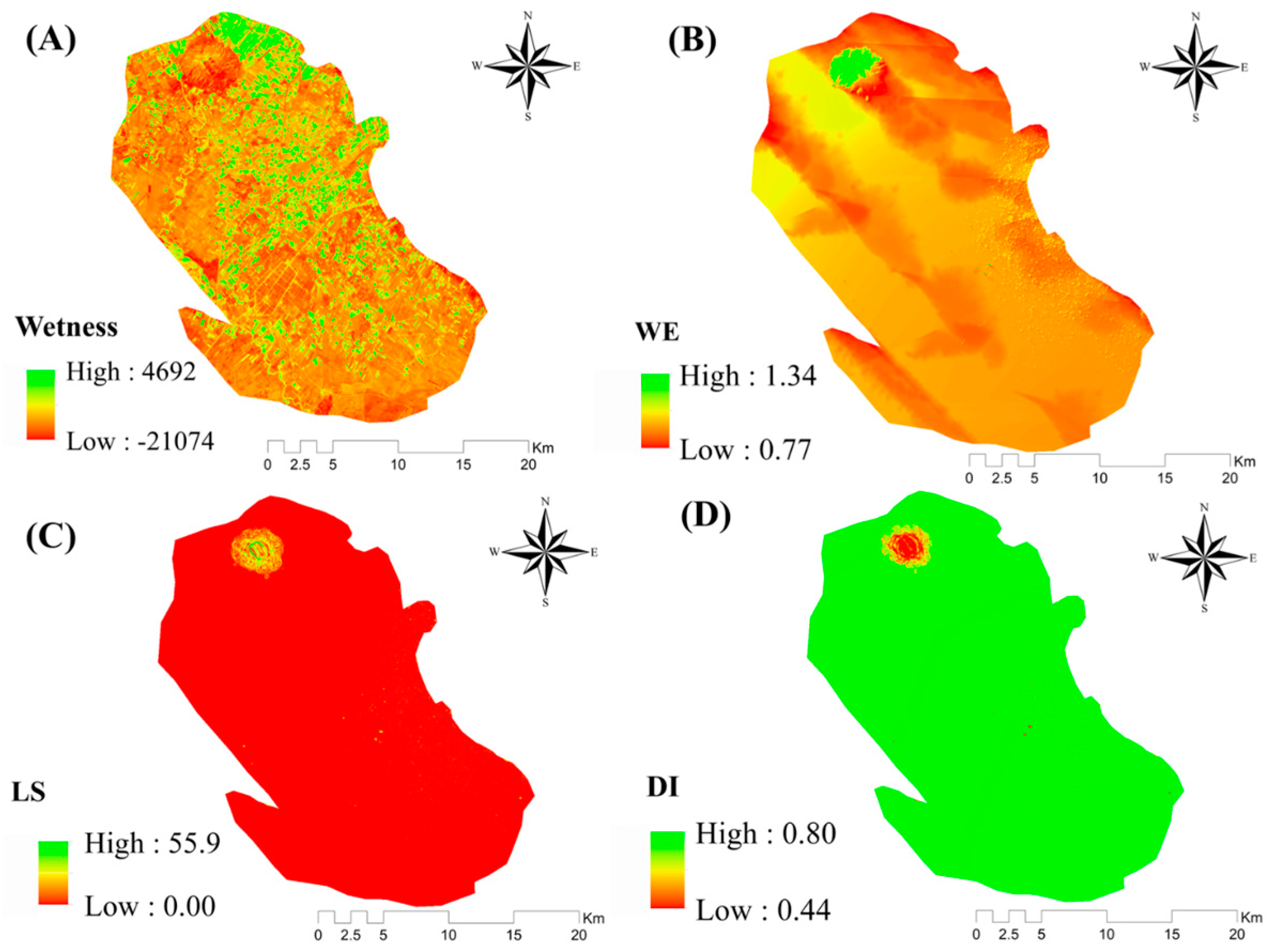
This study aimed to investigate the influence of spatial resolution on the accuracy of soil property predictions. Specifically, we examined how variations in the spatial scale of environmental factors affect the reliability of soil property predictions. To carry out our analysis, we conducted the preprocessing of covariates and prepared a series of spatial resolutions. Before preparing a set of pixel sizes, all the covariates were resampled at the basic 30 × 30 m spatial resolution, and then the other pixel sizes of 60 × 60, 90 × 90, 120 × 120, 150 × 150, 180 × 180, 210 × 210, 240 × 240, 270 × 270, 300 × 300, 330 × 330, 360 × 360, 390 × 390, 420 × 420, 450 × 450, 480 × 480, 510 × 510, 540 × 540, 570 × 570, 600 × 600, 900 × 900, 1200 × 1200, 1500 × 1500, 1800 × 1800, and 2100 × 2100 m were generated by the bilinear interpolation method in the R software platform (4.2.1). It is worth noting that an additional 25 pixel-size series were investigated specifically in the reference area. After determining the pixel size that provided the highest accuracy in predicting the soil properties of interest, the selected scale was used to extrapolate the spatial model to the receptor areas. A total of 22 environmental covariates were gathered and carefully selected through a combination of the recursive feature elimination (RFE) and expert opinion [30] methods. The RFE method, employing a random forest (RF) model, was utilized to determine the most influential covariates among these variables, considering their relationship with soil properties. Ultimately, 11 covariates were identified as highly influential. To provide a visual representation, Figure 2, Figure 3 and Figure 4 showcase the four influential covariates for the reference area and both the first and second receptor areas.

Figure 2.
Spatial distribution of four examples of the most influential environmental factors in the reference area. (A) Wetness: Wetness Index Tasseled Cap Transformation; (B) WE: Wind Effect; (C) LS: LS Factor; (D) DI: Diffuse Insolation.

Figure 3.
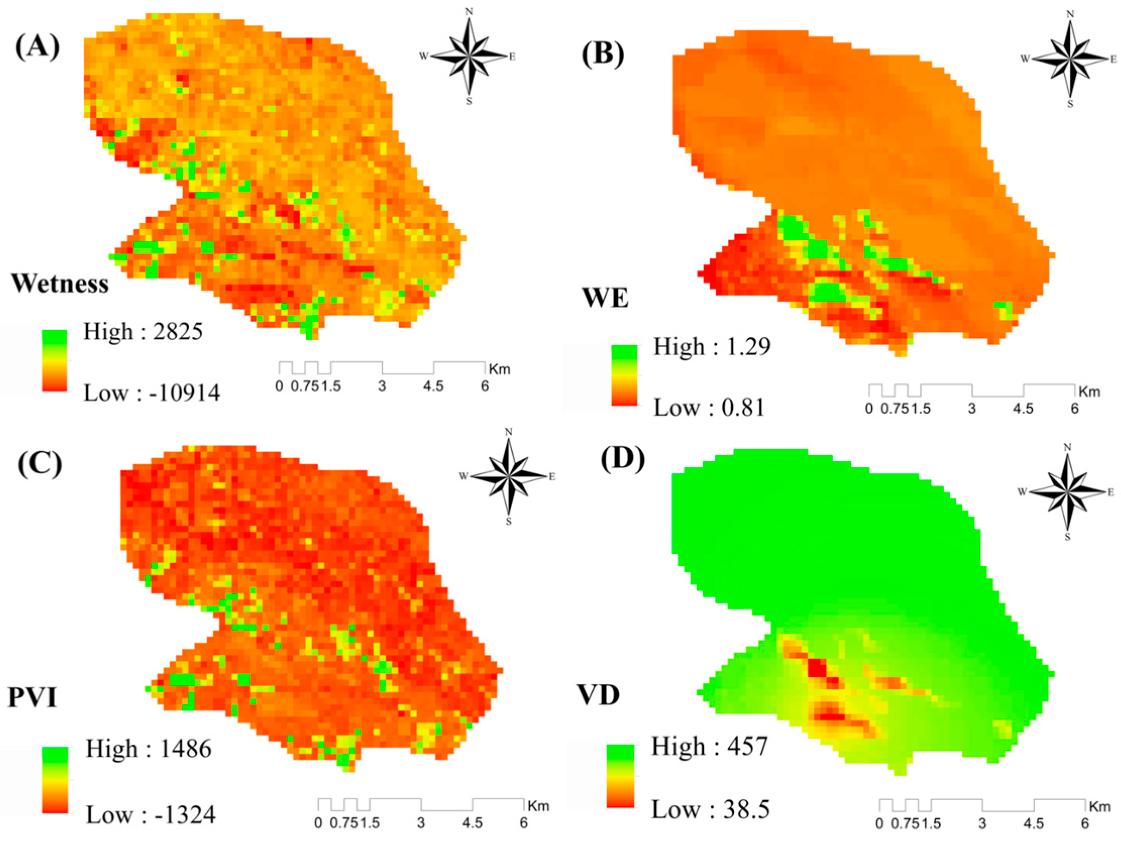
Spatial distribution of four examples of the most influential environmental factors in the first receptor area. (A) Wetness: Wetness Index Tasseled Cap Transformation; (B) WE: Wind Effect; (C) PVI: Perpendicular Vegetation Index; (D) VD: Valley depth.
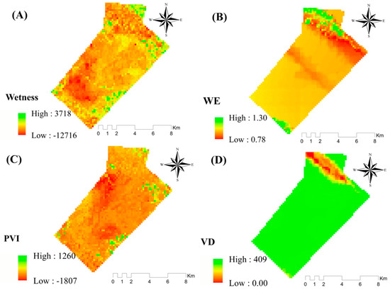
Figure 4.
Spatial distribution of four examples of the most influential environmental factors in the second receptor area. (A) Wetness: Wetness Index Tasseled Cap Transformation; (B) WE: Wind Effect; (C) PVI: Perpendicular Vegetation Index; (D) VD: Valley depth.
2.4. Similarity among Sites
Extrapolating soil maps can be a valuable approach when two areas share similar soil-forming conditions, and the reference area has an adequate number of soil observations to develop prediction models using machine learning techniques [3]. The application of the Homosoil theory [31] provides an opportunity to transfer model results from the reference area to the receptor area, saving time and costs in soil survey projects [21]. In our study, the Marvdasht plain was chosen as the reference area due to its larger size and easier accessibility, while the Bandamir and Lapuee plains served as the receptor areas. Although the three areas exhibit similar climates, parent materials, and topographies, it is essential to quantitatively evaluate their degree of similarity before extrapolation [32]. To assess the similarity between the two areas, we employed the Gower similarity index [33], which considers environmental covariates. For more details about the quantitative and mathematical calculation of similarity index, see [32]. The resulting similarity index ranges from 0 to 1, with values closer to 1 indicating a higher degree of similarity in soil-forming factors. By utilizing the Gower similarity index, we can quantitatively assess the level of similarity between the Marvdasht plain and the Bandamir and Lapuee plains, providing a basis for a proper extrapolation of soil models from the reference to the receptor area.
2.5. Spatial Modeling
This research focused on using modeling techniques to predict four soil properties by optimizing environmental covariates across different scales. The main goal was to examine how scale affects the effectiveness of these covariates in the modeling process and to determine the ideal scale for predicting the targeted soil properties. Additionally, to evaluate model extrapolation in receptor areas, we applied the best-fitting model from the reference area. The optimized environmental covariates were then used at the selected pixel size to predict the four soil properties in the receptor areas by considering SI. Subsequently, we conducted the extrapolation process for these properties in both the primary and secondary receptor areas.
Extreme Gradient Boosting Trees
The XGBoost model was used as the benchmark method for developing regression models linking multiscale covariates to soil properties. XGBoost is a versatile ensemble model based on the tree model, designed for regression and classification predictions [34]. It is known for its scalability and effectiveness, particularly in handling sparse data. This algorithm has found successful applications in soil science, including mapping soil nutrients [5] and other soil properties [35]. XGBoost is a highly effective ML model for modeling and predicting soil properties, particularly due to its ability to optimize hyper parameters [36]. XGBoost provides a wide range of hyper parameters that can be fine-tuned to achieve the best possible model performance for soil property prediction. The hyper parameters in XGBoost allow the tuning of various aspects of the model, and the applied parameters in this research are eta, maximum depth of trees, subsampling ratio, and gamma [37]. By carefully tuning the hyper parameters, there is an opportunity to control the trade-off between model complexity and generalization, ensuring that the XGBoost model captures the intricate relationships within the soil data while avoiding overfitting. Ultimately, all procedures for fitting the XGBoost model were executed using the “caret” and “xgboost” packages, with the assistance of the “xgbTree” function within the R statistical software platform (4.2.1).
2.6. Model Validation
In the process of evaluating the performance of the XGBoost model across various spatial resolution scales within the reference and receptor areas using the cross-validation method, a comprehensive analysis was conducted. This involved the calculation of five widely recognized statistical indices, namely coefficient of determination (R2), Lin’s concordance correlation coefficient (CCC), mean absolute error (MAE), root mean square error (RMSE), and normalized root mean square error (nRMSE). The nRMSE reflects the accuracy of the estimation, with closer values to zero indicating more reliable predictions. These indices were derived using the mathematical formulas represented by Equations (1)–(5), follows Equations (1)–(5):
where ai, bi, , and are the predicted and observed values, and the average of the predicted and observed values over the measurements; r is the correlation coefficient between the predicted and observed values; and , and represent the variance in the predicted and observed values [38].
3. Results
3.1. Summary Statistical of Soil Properties
Table 2 provides a comprehensive overview of the measured soil properties in the reference area and the receptor areas. Descriptive statistics for soil properties (SOM, MWD, BD, and SS) are presented, including the mean, SD, min and max, and CV% values. The mean SOM content is 1.66% in the reference area, 1.71% in the first receptor area, and 1.14% in the second receptor area. Notably, the min and max values of SOM in the reference area vary from 0.22% to 3.22%; furthermore, in the first and second receptor areas, the min and max values vary from 0.62% to 3.79%, and 0.46% to 2.10%, respectively. Also, the mean values of MWD, BD, and SS in the reference, first, and second receptor areas, respectively, are as follows: 2.06 mm, 2.04 mm, 2.25 mm; 1.28 g·cm−3, 1.29 g·cm−3, 1.14 g·cm−3; 2.43 kPa, 2.10 kPa, 1.04 kPa. In addition, in the reference area, the min and max values are as follows: MWD (0.32 mm to 2.43 mm), BD (0.45 gr·cm−3 to 1.79 gr·cm−3), SS (0.14 kPa, to 2.63 kPa). Also, in the first receptor area, the min and max values are as follows: MWD (0.93 mm to 5.50 mm), BD (0.56 gr·cm−3 to 1.87 gr·cm−3), SS (0.50 kPa, to 4.10 kPa); in the second receptor area, the min and max values are as follows: MWD (0.24 mm to 1.64 mm), BD (0.36 gr·cm−3 to 1.95 gr·cm−3), SS (0.10 kPa, to 4.00 kPa).
Table 2.
Descriptive statistics of the four soil properties for the reference (n = 200), first receptor (n = 50), and second receptor (n = 119) areas.
3.2. Selected Environmental Covariates
The optimal environmental covariates were selected using the RFE and expert opinion methods for predicting four soil parameters, namely SOM, MWD, bulk density (BD) and SS, as mentioned in Table 3. In the first phase, the RFE method led to a reduction in the number of environmental covariates from 22 to 11, followed by the inclusion of expert opinion methods to complete the data set of factors. The selected environmental factors can be categorized into two main groups: topography and RS data. As shown in Table 3, the selected factors include six topographic attributes derived from the DEM, consisting of DI, WE, VD, LS, CHNBL, and CND, and five RS variables, namely Brightness, PVI, Wetness, NDVI, and Greenness.
Table 3.
List of the selected covariates for predicting soil properties at the reference and receptor areas.
3.3. Similarity Index
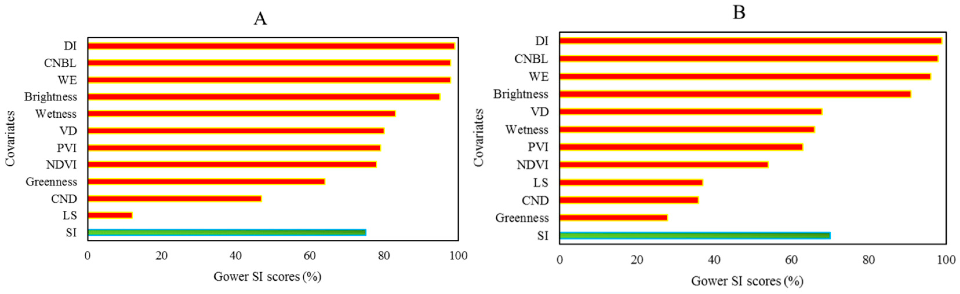
The results for the SI between the reference area and the first receptor area are detailed in Figure 5A, indicating an overall similarity of 76%. Notably, the optimized environmental covariates selected between the reference and first receptor area, such as DI, CNBL, and WE, exhibited high similarity percentages of 99%, 98%, and 98% respectively. The same process was conducted for the comparison of the second receptor region with the first region, yielding an overall similarity index of 70%. According to Gower’s similarity index, this level of similarity (exceeding 70%) supports the extrapolation of predictive modeling procedures to the receptor regions. Furthermore, a significant proportion of the similarity index between the environmental variables in the second receptor area, akin to the first region, was found for DI, CNBL, and WE, with percentages of 99%, 98%, and 96% respectively (Figure 5B). Notably, LS and CND in the first area, and Greenness and LS in the second receptor area, displayed lower similarity rates among all the selected covariates.
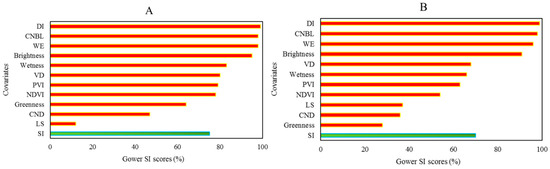
Figure 5.
Gower similarity index: (A) Similarity index of environmental covariates between the reference area and the first receptor area (orange color), along with the overall similarity index of the two areas (green color). (B) Similarity index of environmental covariates between the reference area and the second receptor area (orange color), along with the final similarity index of the two areas (green color). DI = Diffuse Insolation; CNBL = Channel Network Base Level; WE = Wind Effect; Brightness = Brightness; Wetness = Wetness; VD = Valley depth; PVI = Perpendicular Vegetation Index; NDVI = Normalized different vegetation index; Greenness = Greenness; CND = Channel Network Distance; LS = LS-Factor; SI = similarity index.
3.4. Model Validation
3.4.1. Model Validation at Different Scales Scenarios in the Reference Area
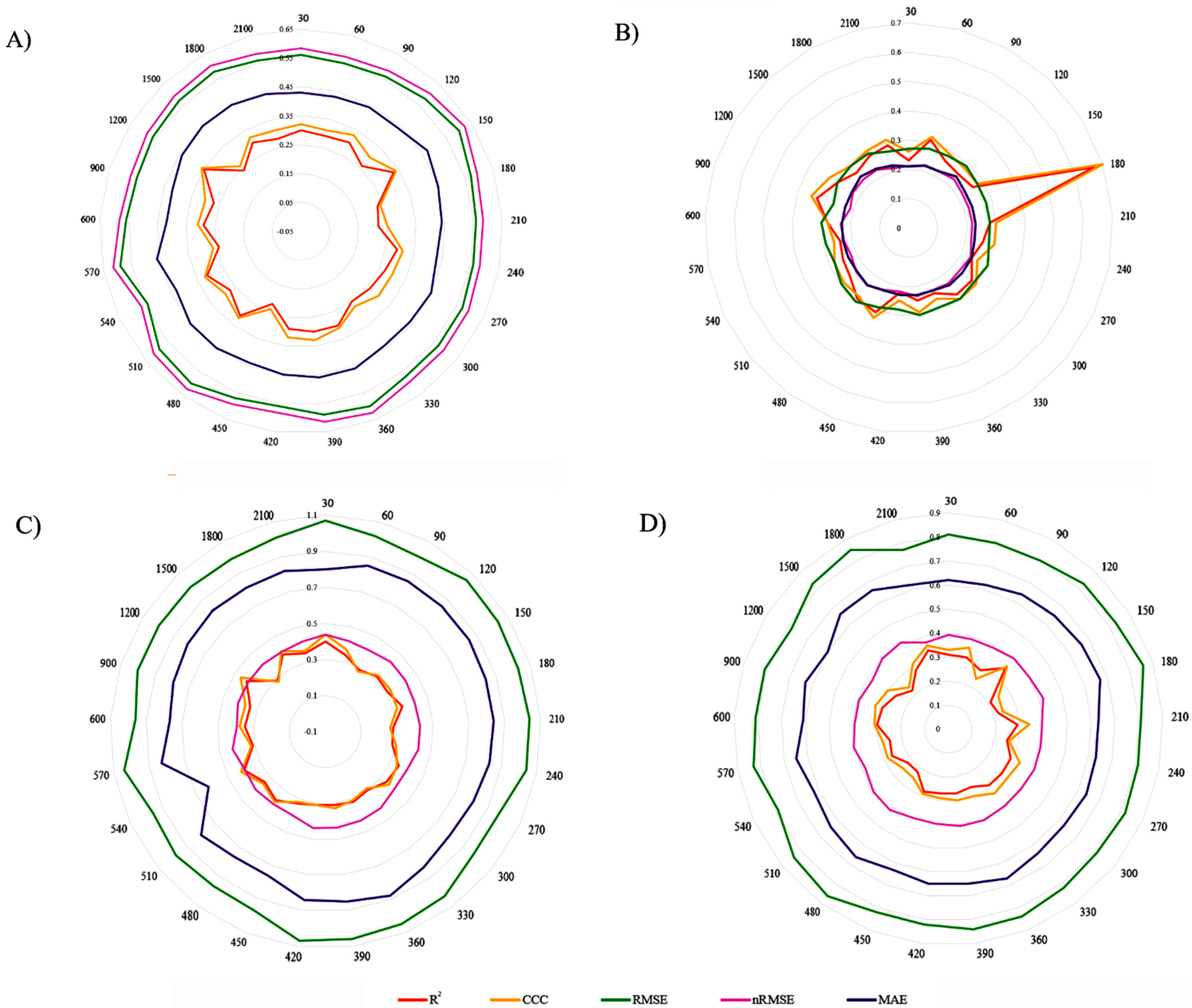
The outcomes of modeling the four soil properties, utilizing the XGBoost ML model, are elucidated in Figure 6, encompassing optimized environmental covariates at 25 scenarios of different scales. Validity statistics, including R2, CCC, RMSE, nRMSE, and MAE, were systematically applied to scrutinize and compare the optimal scales for predicting each of the studied properties. Based on Figure 6A,C, SOM and SS exhibit their optimal performance at the scale of 1200 × 1200 m, reflecting respective statistical measures of R2 (0.35, 0.42) and CCC (0.36, 0.46), respectively. The validation outcomes for MWD indicate that its optimal performance is achieved at the scale of 2100 × 2100 m, given the R2 and CCC values of 0.34 and 0.36, respectively. These results affirm that the 2100-meter scale outperforms other scales in the prediction of MWD in the reference area. For BD, the optimal scale was found in 180 × 180 m pixel resolution. The validation results also revealed R2 = 0.67 and CCC = 0.70 for BD in this scale scenario (Figure 6B). Based on the accuracy metric, the overall trend in soil property validation indicates a fluctuating trend. However, for SS and MWD, there is a consistent pattern from the basic scale of 30 m to 90 m, followed by an increase from 240 m to 300 m. Subsequently, from 330 m to 450 m, there is a slight consistency, and beyond 1200 m, SS shows an increasing trend, while MWD exhibits a decreasing trend (Figure 6D). Conversely, for SOC and BD, there is an inverse trend from the basic scale of 30 m to 450 m, but beyond 450 m, they display a converging trend until 2100 m (Figure 6A,B).
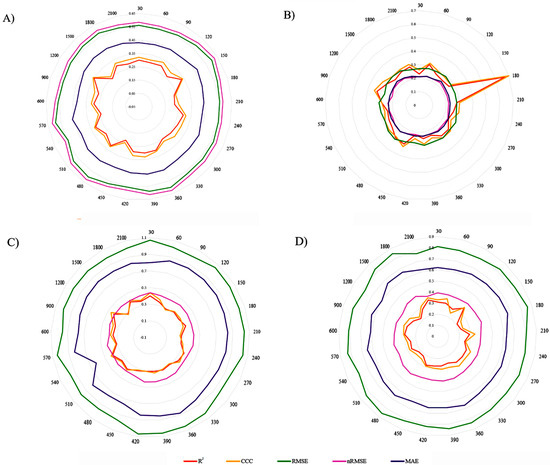
Figure 6.
Validation results of soil properties in different pixel sizes in the reference area (interpolation). (A) SOM = soil organic matter; (B) BD = bulk density; (C) SS = shear strength; (D) MWD = mean weight diameter of aggregates; R2: coefficient of determination; RMSE: root mean squared error; nRMSE: normalized root mean squared error; CCC: concordance correlation coefficient; MAE: mean absolute error.
Based on the findings presented in Figure 6, it can be observed that SOM and SS demonstrated their best performance when applied at the scale of 1200 × 1200 m. This was evidenced by the respective statistical measures of R2 (0.35, 0.42) and CCC (0.36, 0.46). Additionally, the validation results for MWD indicated that its optimal performance was achieved at the scale of 2100 × 2100 m, with R2 and CCC values of 0.34 and 0.36, respectively. Furthermore, the optimal scale for BD was determined to be at a pixel resolution of 180 × 180 m, with validation results showing R2 = 0.67 and CCC = 0.70.
3.4.2. Model Validation in the Receptor Area (First and Second Receptor Areas)
Based on the identified best predictive scale (see Table 4 and Table 5), Table 4 presents the validation outcomes for soil properties at the first receptor area, using diverse metrics to evaluate the model’s predictive performance. It was observed that SOM and SS at the optimal scale of 1200 × 1200 m showed moderate fitting with (R2 = 0.46, 0.50) and (CCC = 0.51, 0.55), respectively, indicating acceptable agreement between predicted and observed values [39]. In contrast, MWD predictions at a scale of 2100 × 2100 m exhibited a good fit (R2 = 0.65, CCC = 0.70), implying predictions with higher accuracy. The validation results for BD at the optimal scale of 180 × 180 m with (R2 = 0.25 and CCC = 0.30) showed weak accuracy in the first extrapolation area.
Table 4.
The validation result of the four soil properties at the first receptor area.
Table 5.
The validation results of the four soil properties at the second receptor area.
Table 5 displays the validation results for soil properties at the second receptor area, using a range of metrics to evaluate the accuracy of the predictive model. For SOM and SS at a scale of 1200 × 1200 m, the model demonstrates a strong fit with R2 values ranging from 0.58 to 0.64 and CCC values ranging from 0.62 to 0.68. The predictions for MWD at a scale of 2100 × 2100 m indicate a moderately strong fit (R2 = 0.60, CCC = 0.65), suggesting accurate predictions. Additionally, BD predictions at a scale of 180 × 180 m show an acceptable fit (R2 = 0.52, CCC = 0.54), indicating a moderate level of accuracy. These results collectively provide insight into the model’s performance in predicting soil properties at different scales in the second receptor area. Importantly, all extrapolation models for the soil properties, except BD, demonstrated higher accuracy in the receptor areas compared to the reference area. A similar observation was made by Khosravani et al. [3] in their extrapolation modeling of soil fertility properties when applying covariates with a 30 m spatial resolution.
3.5. Covariate Importance
Figure 7 provides a comprehensive evaluation of various pixel sizes of covariates, illustrating their relative importance in predicting soil properties. Notably, these environmental covariates play a key role in the prediction of soil properties of interest.
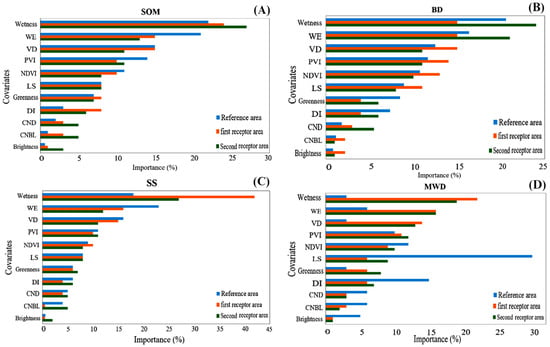
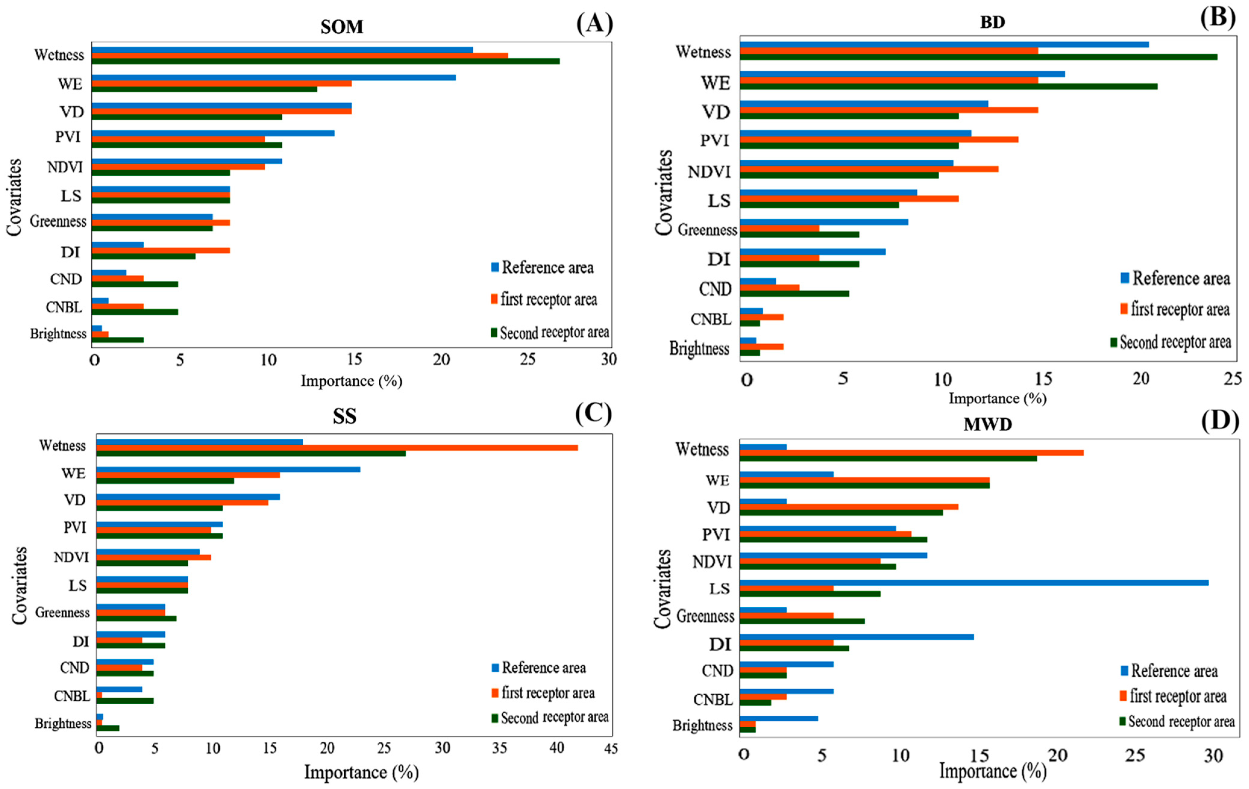
Figure 7.
The relative importance of the selected environmental covariates at the reference, first, and second receptor areas. (A) SOM = soil organic matter. (B) BD = bulk density. (C) SS = shear strength. (D) MWD = mean weight diameter of aggregates. Wetness = Wetness; WE = Wind Effect; VD = Valley depth; PVI = Perpendicular Vegetation Index; NDVI = Normalized different vegetation index; LS = LS-Factor; Greenness = Greenness; DI = Diffuse Insolation; CND = Channel Network Distance; CNBL = Channel Network Base Level; Brightness = Brightness.
3.5.1. Covariate Importance in the Reference Area
Figure 7 presents the relative importance of selected environmental covariates in predicting BD, MWD, SOM, and SS in the reference area. In Figure 7A–C, Wetness, WE, VD, and PVI account for 70%, 65%, and 62% of the total variation of SOM, SS, and BD, respectively, making them the top four covariates in predicting BD. Conversely, for MWD, the LS, DI, NDVI, and PVI account for 70% of its total variation, as shown in Figure 7D. The multiscale covariates, such as Wetness, WE, VD, and PVI, exhibit a remarkable ability to maintain their influence across a wide spectrum of resolutions, from finer to coarser. This is particularly evident in their impact on the prediction of soil properties. For example, the influence of these covariates is observed in the prediction of BD at a resolution as fine as 180 × 180 m. Furthermore, their influence is also significant in the prediction of SOM and SS at a resolution as coarse as 1200 m. This finding underscores the robust and versatile nature of these covariates in contributing to the accurate prediction of soil properties across varying spatial scales [40].
The top three covariates Wetness, NDVI, and PVI are positioned among the top-ranking variables and are sourced from RS. Also, it is very notable that the WE, DI, VD, and LS as topographic attributes along with RS covariates displayed high-frequency roles in the prediction of soil properties at the different-scale scenarios. This study shows that the terrain attributes had the highest overall contribution to the prediction of soil properties, highlighting the importance of landscape characteristics in spatial variability.
3.5.2. Covariate Importance in Receptor Areas (First and Second Receptor Areas)
After analyzing the modeling results in the extrapolation areas (first and second receptor areas), we investigated the significance of the optimized environmental covariates for predicting soil properties in these regions. The findings indicated that for each of the four soil properties studied (BD, SOM, SS, MWD) in the first receptor area, the extrapolation of the environmental variables Wetness and WE had the highest RI in predicting these properties. Following these two environmental covariates, two other covariates, namely VD and PVI, also demonstrated significant importance in predicting all four traits (refer to Figure 7). The results for the RI of predictive environmental covariates for the second extrapolation region were similar to those of the initial extrapolation region (refer to Figure 7). In this context, it is important to note that the four covariates (Wetness, WE, VD, and PVI) hold the same level of significance as the reference area. Their relevance can be highly attributed to their similarity with the reference area, with a mean similarity of 81% for the first receptor area and 73.25% for the second receptor area (see Figure 7). Therefore, this finding verified that attributes like Wetness, WE, VD, and PVI are the key factors influencing the distribution of soil properties in the semiarid region. It is important to recognize the significance of these attributes and not overlook them in future predictions of the desired soil properties.
3.6. Spatial Prediction
3.6.1. Spatial Prediction Maps in the Reference Area
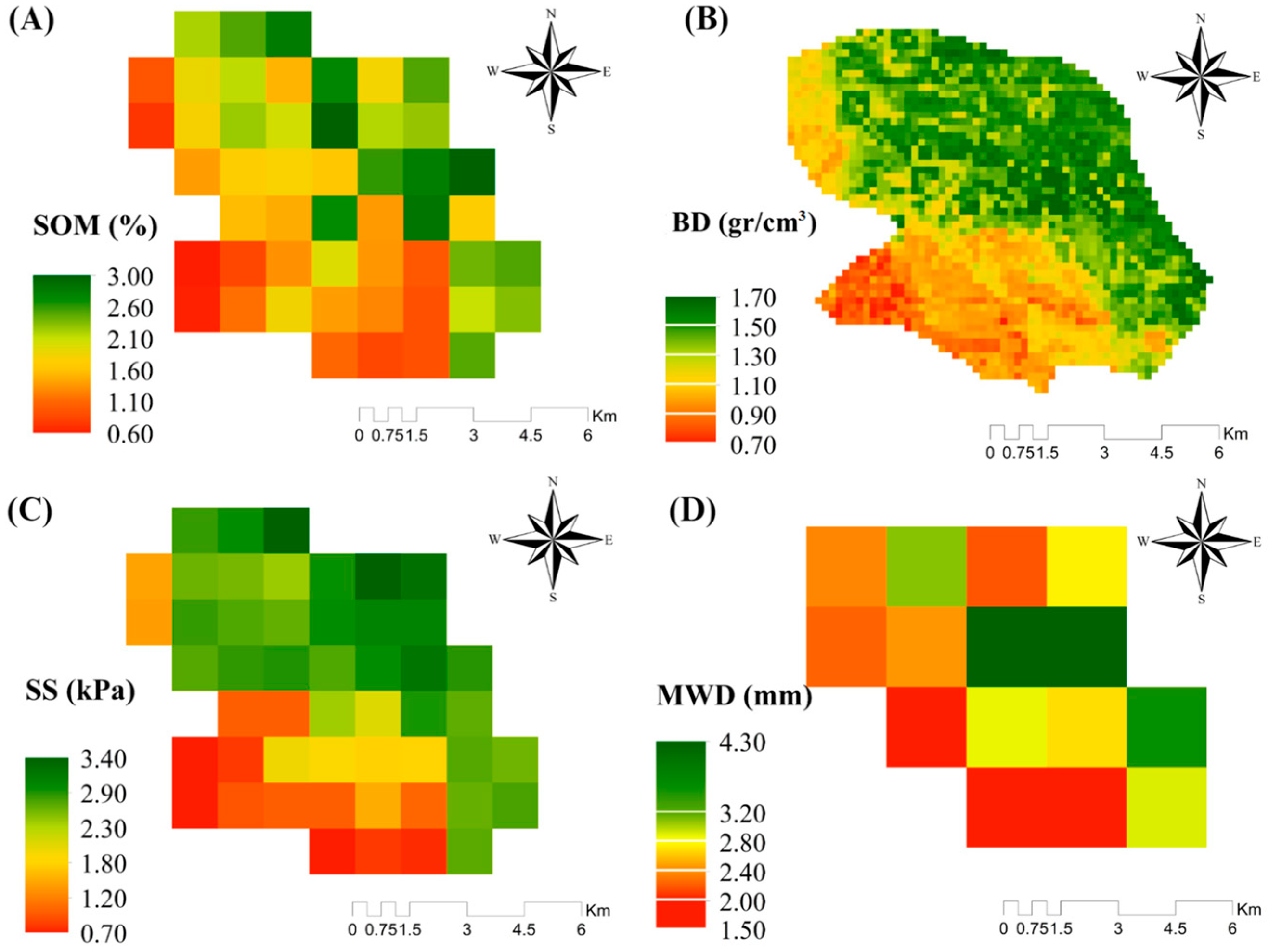
The best prediction model pixel size (Figure 6) was used to generate the spatial prediction maps of the soil properties of interest in the reference area (Figure 8). Figure 8A shows that the spatial prediction of SOM and the maps are relatively homogeneous from the northern to the southern part of the study area, with a range from 0.9% to 2.50%. For BD, the minimum contents in the northern to northeastern part is BD < 1 gr·cm−3, and the maximum values in the southeastern and western parts are between 1.5 gr·cm−3 and 1.75 gr·cm−3 (Figure 8B). The MWD content between 2.40 mm and 3.20 mm dominated, showing considerable stability without encrusted soils, especially in the central and southern parts (Figure 8D). In addition, the SS content varied between 0.33 kPa and 4.00 kPa, with the maximum content in the center to the west and minimum content in the north to northeast region (Figure 8C). Considering the main covariates in predicting SOM, BD, and SS, their maximum competition is relatively closely followed by minimum values of WE and medium to low values of Wetness (Figure 2).
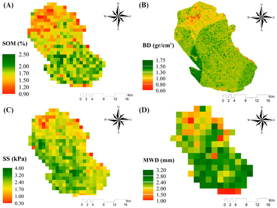
Figure 8.
The spatial prediction maps of soil properties at the best scale scenario in the reference area. (A) SOM = soil organic matter; (B) BD = bulk density; (C) SS = shear strength; (D) MWD = mean weight diameter of aggregates.
3.6.2. Spatial Prediction Maps in the Receptor Areas
First Receptor Area
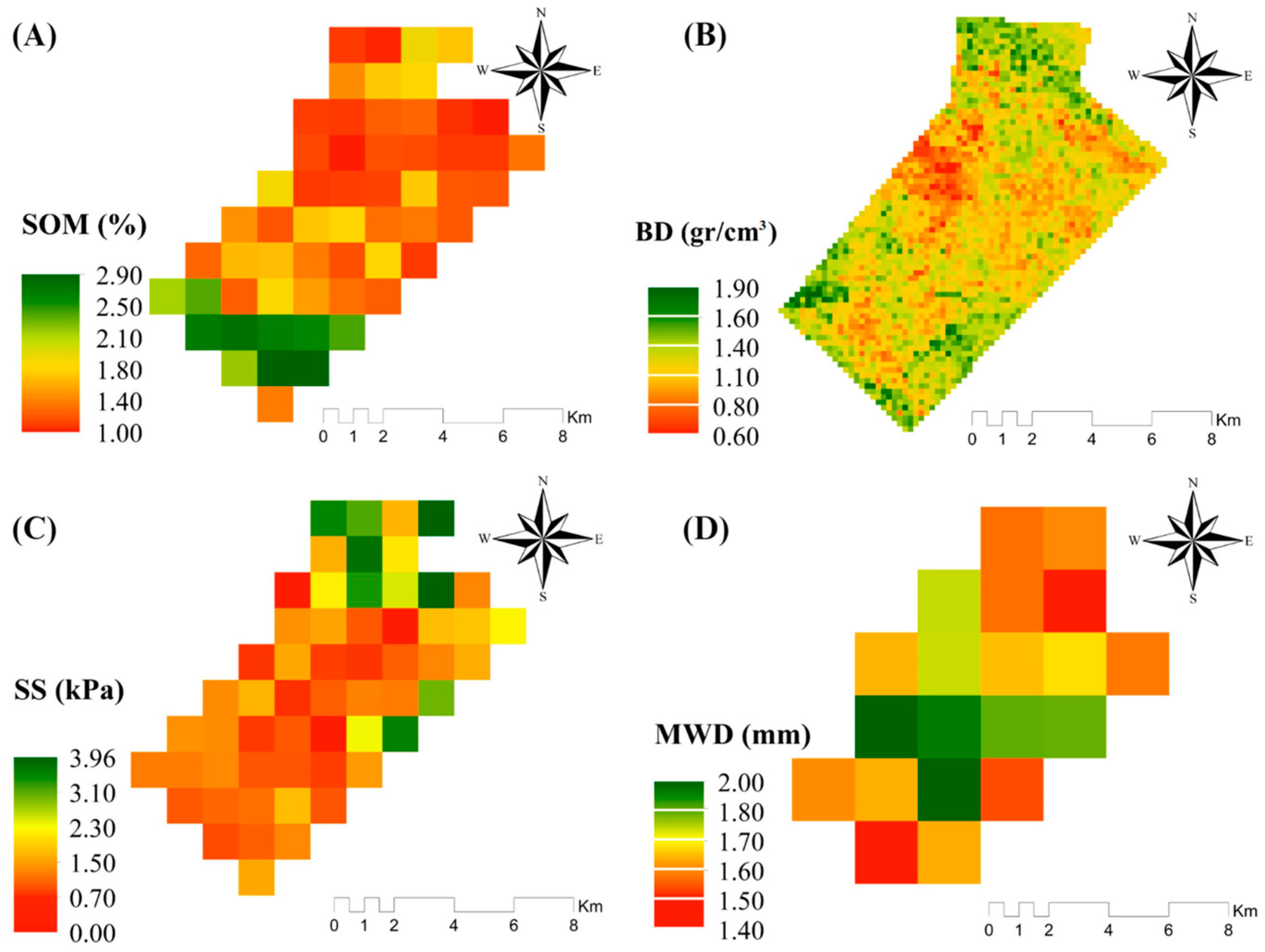
The generation of a spatial prediction map for soil properties in the first receptor area delineated that for each of the three properties (SS, SOM, and BD), the maximal values were observed in the northeastern, eastern, southeastern, and central sectors (Figure 9). As one traversed towards the western, southwestern, and northwestern regions, a gradual decrement in the magnitudes of these attributes within the study area became evident. For MWD, it was noted that the augmentation of scale during the modeling process led to the omission of specific areas within the study area from the ultimate predictive map of this properties. Furthermore, noteworthy magnitudes of these properties were solely evident in selected central and southwestern regions, while registering comparatively diminished levels in other sectors, particularly the western and southern areas. Therefore, an important point that should be considered regarding the first receiving area in scale and generalization studies is that if the goal is to use maps for detailed management, the area of the study area and the amount of detail that is possibly neglected by increasing size of the pixel should be taken into consideration.

Figure 9.
The spatial extrapolation maps of soil properties at the best scale scenario in the first receptor area. (A) SOM = soil organic matter; (B) BD = bulk density; (C) SS = shear strength; (D) MWD = mean weight diameter of aggregates.
Second Receptor Area
The spatial predictive map of soil attributes in the second area reveals that for MWD, predominantly modest to low values were observed across most regions, with an increase discernible only in specific central areas (Figure 10D). Importantly, it is worth noting that, akin to the first receptor area, the modeling at an elevated scale resulted in the omission of certain areas within the study region from the generated predictive map. SS displayed predominantly modest to low values across all study areas, with noteworthy elevations observed solely in specific northern and southern sectors of the designated area (Figure 10C). Similarly, SOM exhibited relatively subdued values across the majority of areas, experiencing a conspicuous increase only in the southwestern areas of the specified area (Figure 10A). Finally, BD demonstrated moderate values throughout most points within the study domain, with particularly elevated values discernible in certain northern, southern, and southwestern areas. Furthermore, the minimum values of BD were identified in specific northwestern areas (Figure 10B).
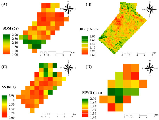
Figure 10.
The spatial extrapolation maps of soil properties at the best scale scenario in the second receptor area. (A) SOM = soil organic matter; (B) BD = bulk density; (C) SS = shear strength; (D) MWD = mean weight diameter of aggregates.
4. Discussion
According to Charman and Roper [41], the studied soils had a severely low SOM content; also, based on the Le Bissonnais [42] classification, the mean of the MWD of soil has shown considerable stability with no crusting. MWD, as a key indicator of soil aggregate stability, plays a crucial role in soil conservation and the preservation of its environmental functions [43], as well as in the storage and stabilization of organic carbon [44]. The CV% for SOM and BD indicates moderate variability, while MWD and SS exhibit significant variability across all three regions, as per the classification by Wilding and Dress [45]. The substantial variability in agricultural soils is primarily associated with anthropogenic factors, such as land use type and management decisions, which can influence the variability of soil properties [46].
In this regard, researchers believe that a carefully selected subset of covariates generally performs better than using all available covariates for mapping soil properties [30]. Terrain attributes were the main predictors among different studied auxiliary information and are the key influential parameters in the prediction of soil properties [47]. So, selecting the optimal scale of environmental covariates is extremely crucial in model validation and reduces uncertainty by increasing the quality of predictions.
The findings in this study indicate that the highest accuracy of SOM and SS mainly rely upon a larger scale (more than 1000 m) of environmental covariates, while for MWD and BD, their accuracy is mostly dependent upon small resolutions. In a case study in Denmark by Zhang [48], it was found that a pixel size of 88 m, as compared to 30.4 m and 92.8 m, resulted in a higher accuracy in predicting soil organic carbon. The study area, being relatively flat, showed a strong relationship between model performance and grid resolution. In this regard, Cavazzi [16] observed that in flat, homogeneous areas, coarser resolutions (>140 m) were preferred, while morphologically varied terrain favored finer resolutions (30 m). The primary factor influencing the spatial variability of bulk density (BD) is soil organic matter (SOM). Additionally, land use and elevation play significant roles in affecting soil BD variability. The soil genus is also crucial in this context. Furthermore, soil management practices and tillage activities contribute to considerable variability in soil BD [49] at a fine scale, complicating its spatial distribution even further. Similarly, Dornik [19] observed a significant increase in R2 values and a decrease in RMSE when predictors are at their optimal scale, rather than at a basic scale, in the prediction of soil properties. Notably, the XGBoost model exhibited limitations in accurately predicting some soil properties (SOM, SS, and MWD), as indicated by its low R2 values. Interactions among environmental covariates occur at multiple scales, influencing the genesis and spatial dependencies of soil and other environmental properties [50]. The effect of multiscale predictions in soil identification and terrain analysis emphasizes the importance of integrating various covariates across different resolutions. In mountainous regions, topographic features such as elevation, slope, aspect, and curvature can effectively distinguish soil types due to their pronounced influence on soil formation processes [51]. However, in more complex geomorphological areas like plains and hilly terrains, relying solely on these individual features may not capture the intricate interactions affecting soil variability [52].
To extrapolate modeling results from a reference area to the receptor areas, it is crucial to initially evaluate the SI of the environmental covariates between the reference and receptor areas [53]. This underscores the substantial similarity between the two areas, providing a foundation for extending the modeling results to other areas [54]. In contrast to our results, the authors of [11] did not find high Homosoil scores (SI) among a set of reference areas and a receptor area in their studies at the country level in Africa.
The Wetness, NDVI, and PVI variables are instrumental in reflecting the moisture content of soil and plants [55], as well as the structural characteristics of vegetation and level of canopy cover [56]. NDVI is a crucial factor for predicting SOC in flatlands, as it serves as an indicator of crop growth and biomass, making it a reliable proxy for SOC prediction [48]. Moreover, multiple studies have highlighted the significance of variables representing the ‘organisms’ factor within the SCORPAN method as crucial covariates in the prediction of soil properties [57].
With regard to topographic attributes, our findings are consistent with previous research by Kumaraperumal [58], who also reported a strong correlation between relief parameters and soil properties. In a research work [48], the authors found that topographic attributes have different contributions according to pixel size in the prediction of soil properties. They observed that the relative slope position and elevation are the most important attributes in the prediction of SOC at a resolution between 30 m and 250 m, while, VD should be selected at a resolution finer that 30 m or coarser than 250 m. Furthermore, Minasny [59] and Adhikari [60] reported that topographical attributes play key roles in the prediction of SOC at the national and global scales. Similarly, Guo [61] found that when modeling SOC distribution, three terrain attributes—relative slope position, channel altitude, and standard height—were identified as the most significant across all resolutions. These variables should be considered critical in future DSM studies. Additionally, VD was recognized as another important covariate that is scale-dependent. Although this research did not utilize direct proxies for parent materials and ages, certain topographic attributes, such as VD, significantly influence hydrological, erosional, and depositional processes [62]. These attributes can indicate the types of materials that have accumulated over time, including sediments from surrounding areas. Furthermore, WE demonstrates the potential for particulate matter to be transported from source areas. The accumulation of secondary carbonates within the soil profile is a common occurrence [63], highlighting their multifunctional role in the landscape.
Accordingly, Keshavarzi [64] investigated the distribution of soil physical properties (BD and SS) in relation to topography. The lower SS (Figure 8C) in the reference area observed in northern regions is primarily due to the influence of mountainous and piedmont physiographic features. In contrast, areas with low relief, such as alluvial plains, tend to exhibit higher SS. Elevated terrains often have a compromised soil structure, reduced SOM, increased erosion rates, and diminished resistance to cutting. Field observations indicate that severe erosion, along with the presence of stones and gravel, contributes to a fragile soil structure at greater depths, resulting in a decline in SS from the surface downwards [65]. According to Table 3 and Figure 8B, the mean value of BD is 1.28 g·cm−3 in the reference area, and this variation trend can be seen in most parts of the study area. Referring to Figure 7 (BD), the variables Wetness, WE, VD, and PVI emerged as key covariates in predicting BD. Their variation is primarily linked to vegetation and topographic attributes. Since most of the study area is under irrigation for crops, albeit not consistently, the type of vegetation significantly influences BD variability. Vegetation and environmental factors significantly influence apparent BD by affecting soil structure, SOM, and compaction levels. Dense vegetation and extensive root systems typically result in lower BD due to the increased pore space and contributions of SOM. Conversely, soil compaction caused by mechanical activities or dry conditions can lead to an increase in bulk density [66]. Also, topographic attributes influence the rate and direction of the movement of water through landscapes and dictate erosion and deposition patterns [40], leading to the accumulation of water as indicated by terrain indices that determine the distribution of vegetation cover [67]. For SOM and SS, in Figure 9, it can be observed that they have similar spatial distribution, although based on Charman and Roper [41], the SOM content in these soils is at a low or very low level in most parts of the study area. In our study area, the low content of SOM is reminiscent of the conditions observed in semi-arid regions, where high temperatures significantly enhance soil biological activity. This increase in activity accelerates the degradation of SOM, leading to a reduction in microbial biomass and dissolved SOM. Boudjabi and Chenchouni [68] highlight that these changes are often associated with reduced plant litter fall, which further exacerbates the decline in SOC levels. Moreover, the management practices employed by farmers play a crucial role in influencing SOC dynamics. The evidence indicates that the spatial variability of SS is highly dependent on RS and topographic attributes. In this regard, Wall [69] found that the Sentinel-2 satellite bands B1, B2, and B3 significantly predicted SS. This study highlights the relationship between SS and vegetation attributes, demonstrating the feasibility of linking SS to RS variables through a multivariate model. Ghavami [70] reported that some topographical characteristics (VD, catchment area, multi-resolution of ridge top flatness index) and some soil characteristics (i.e., clay, SOM, and MWD) were the most important input variables for predicting SS in semi-arid regions of Iran. In Figure 9C, the area for BD is primarily situated on a piedmont plain with a heavy soil texture, except for the southwestern region. In other parts of the study area, BD exhibits significant variability and an erratic pattern. According to Li [49], this variability is mainly influenced by fluctuations in soil moisture and hydraulic conductivity. These factors are essential for evaluating soil quality and effectively managing land use. For SOM, solar radiation varies depending on orientation, which affects vegetation and evaporation [71]. Overall, these factors lead to complex feedback in the development of the catena with the accumulation or degradation of SOC. The spatial distribution of MWD is also closely related to the highest values of DI and the lowest values of LS (Figure 2). In addition to DI and LS as topographic attributes, NDVI and PVI as proxy vegetation indices play important roles in predicting MWD. Similarly, Jin [72] observed that topography indirectly affects MWD through its influence on the vegetation cover of the land. Moreover, vegetation serves as a source of SOM that directly contributes to the formation and stabilization of aggregates [73]. In conclusion, the stability of soil aggregates is significantly influenced by soil properties and the percentage of vegetation cover in the studied areas.
5. Research Strengths and Weakness/Limitations
5.1. Strengths
Effective Use of Machine Learning: The application of the XGBoost ML algorithm demonstrated acceptable predictive accuracy for soil properties, particularly for SOM, SS, and MWD, indicating the model’s robustness in spatial modeling. Optimal Pixel Size Identification: This research identified optimal pixel sizes for different soil properties, enhancing the precision of soil mapping and informing future studies on pixel size selection for environmental monitoring. Knowledge Transfer: This study successfully applied the Homosoil framework, achieving high SI scores between reference and receptor areas, which supports effective knowledge transfer in soil property modeling. Cost and Time Efficiency: By utilizing optimal pixel sizes and the Homosoil framework, this research offers the potential for time and cost savings in soil survey projects, particularly in regions with limited data.
5.2. Weakness/Limitations
Limited Scope of Soil Properties: This study primarily focused on a few soil properties (SOM, BD, SS, MWD), which may not represent the full spectrum of soil characteristics relevant for comprehensive land management. Resolution Dependency: The findings indicate that BD shows higher accuracy at finer resolutions, suggesting that important details may be overlooked at coarser resolutions, potentially affecting the overall soil property assessment. Generalizability Concerns: While this study extrapolated findings to other plains, the applicability of the results to different geographical areas or soil types may be limited, necessitating further validation in diverse contexts. Exclusion of Direct Covariates: This research did not utilize direct covariates as proxies for parent materials, age, climatic data, and legacy soil data. This limitation may restrict the understanding of the underlying soil formation processes and may reduce the accuracy of predictions related to soil properties. Uncertainty of Prediction: Uncertainty assessment is a crucial aspect of predictive modeling. In a spatial context, the reliability of predictions generated by statistical or machine learning models can vary significantly across different locations [74].
6. Conclusions
This research aimed to identify key terrain attributes and RS indices for the spatial modeling of four soil properties, namely SOM, BD, SS, and MWD, using the XGBoost ML algorithm. This study found that SOM, SS, and MWD were primarily influenced by larger pixel sizes, while BD was more accurately represented at finer resolutions. High accuracy for SOM, SS, and MWD was achieved at coarser resolutions (1800 m, 1800 m, and 2100 m), whereas BD was most accurate at 180 m. All soil properties showed improved accuracy beyond their original pixel sizes (30 m). These findings can guide the selection of appropriate pixel sizes for accurate soil property mapping, enhancing environmental monitoring and land management practices. In terms of knowledge transfer between the reference and receptor areas, the application of the Homosoil framework revealed that the receptor areas achieved overall similarity index scores of 76% and 70% for the first and second receptor areas, respectively. The validation results of the extrapolated model displayed higher accuracy (as measured by R2) in the receptor areas compared to the reference area, with the exception of BD. Beyond the validation quality, an important point that should be taken into account regarding the first and second receptor areas in scale and extrapolation studies is as follows: if the objective is to use maps for detailed management, then the extent of the study area and the amount of detail that is possibly neglected/omitted by increasing the pixel size should be taken into consideration for future work (i.e., MWD and SOM maps in the first and second receptor areas). The assessment of the RI of environmental covariates for the selected soil properties indicated that topographic attributes (such as WE, VD, LS) and RS indices (Wetness, PVI, and NDVI) played a major role in the reference area. Conversely, CHNBL and Brightness had lower importance in the ranking of environmental covariates. The receptor areas showed similar trends, with WE, VD, Wetness, and PVI identified as the most important covariates. In conclusion, the joint utilization of optimal pixel sizes for environmental covariates and the Homosoil framework can lead to time and cost savings in soil survey projects, particularly in areas with limited soil data, as is the case in many parts of Iran.
Author Contributions
Conceptualization, P.K.; methodology, P.K. and S.R.M.; software, P.K., S.R.M., and A.A.M.; validation, P.K. and S.R.F.S.; formal analysis, P.K. and N.M.K.; resources, S.R.M.; data curation, P.K.; writing—P.K.; writing—review and editing, T.S. and R.T.-M.; visualization, H.S.; supervision, M.B. and T.S.; project administration, M.B. and T.S. All authors have read and agreed to the published version of the manuscript.
Funding
This study was supported by “Shiraz University, and Faculty of Agriculture”.
Data Availability Statement
Data are available upon reasonable email request to the corresponding author. The data are not publicly available due to ethical reasons.
Acknowledgments
The authors express their deep gratitude to Shiraz University for providing the financial support necessary to conduct this research. They also extend their sincere appreciation to the editor and reviewers involved in the publication process.
Conflicts of Interest
The remaining authors declare that the research was conducted in the absence of any commercial or financial relationships that could be construed as potential conflicts of interest.
References
- Li, J.; Nie, M.; Powell, J.R.; Bissett, A.; Pendall, E. Soil physico-chemical properties are critical for predicting carbon storage and nutrient availability across Australia. Environ. Res. Lett. 2020, 15, 094088. [Google Scholar] [CrossRef]
- Kv, U.; Km, R.; Naik, D. Role of soil physical, chemical and biological properties for soil health improvement and sustainable agriculture. J. Pharmacogn. Phytochem. 2019, 8, 1256–1267. [Google Scholar]
- Khosravani, P.; Baghernejad, M.; Moosavi, A.A.; FallahShamsi, S.R. Digital mapping to extrapolate the selected soil fertility attributes in calcareous soils of a semiarid region in Iran. J. Soils Sediments 2023, 23, 4032–4054. [Google Scholar] [CrossRef]
- Fathololoumi, S.; Vaezi, A.R.; Alavipanah, S.K.; Ghorbani, A.; Saurette, D.; Biswas, A. Improved digital soil mapping with multitemporal remotely sensed satellite data fusion: A case study in Iran. Sci. Total Environ. 2020, 721, 137703. [Google Scholar] [CrossRef]
- Hengl, T.; Leenaars, J.G.; Shepherd, K.D.; Walsh, M.G.; Heuvelink, G.B.; Mamo, T.; Tilahun, H.; Berkhout, E.; Cooper, M.; Fegraus, E.; et al. Soil nutrient maps of Sub-Saharan Africa: Assessment of soil nutrient content at 250 m spatial resolution using machine learning. Nutr. Cycl. Agroecosyst. 2017, 109, 77–102. [Google Scholar] [CrossRef]
- Eymard, A.; Richer-de-Forges, A.C.; Martelet, G.; Tissoux, H.; Bialkowski, A.; Dalmasso, M.; Chrétien, F.; Belletier, D.; Ledemé, G.; Laloua, D.; et al. Exploring the untapped potential of hand-feel soil texture data for enhancing digital soil mapping: Revealing hidden spatial patterns from field observations. Geoderma 2024, 441, 116769. [Google Scholar] [CrossRef]
- Richer-de-Forges, A.C.; Chen, Q.; Baghdadi, N.; Chen, S.; Gomez, C.; Jacquemoud, S.; Martelet, G.; Mulder, V.L.; Urbina-Salazar, D.; Vaudour, E.; et al. Remote sensing data for digital soil mapping in French research—A review. Remote Sens. 2023, 15, 3070. [Google Scholar] [CrossRef]
- Mulder, C.; Boit, A.; Bonkowski, M.; De Ruiter, P.C.; Mancinelli, G.; Van der Heijden, M.G.; Van Wijnen, H.J.; Vonk, J.A.; Rutgers, M. A belowground perspective on Dutch agroecosystems: How soil organisms interact to support ecosystem services. In Advances in Ecological Research; Academic Press: Cambridge, MA, USA, 2011; Volume 44, pp. 277–357. [Google Scholar] [CrossRef]
- Bell, L.W.; Kirkegaard, J.A.; Swan, A.; Hunt, J.R.; Huth, N.I.; Fettell, N.A. Impacts of soil damage by grazing livestock on crop productivity. Soil Tillage Res. 2011, 113, 19–29. [Google Scholar] [CrossRef]
- Ben-Dor, E.; Taylor, R.G.; Hill, J.; Demattê, J.A.M.; Whiting, M.L.; Chabrillat, S.; Sommer, S. Imaging spectrometry for soil applications. Adv. Agron. 2008, 97, 321–392. [Google Scholar] [CrossRef]
- Hateffard, F.; Steinbuch, L.; Heuvelink, G.B.M. Evaluating the extrapolation potential of random forest digital soil mapping. Geoderma 2024, 441, 116740. [Google Scholar] [CrossRef]
- McBratney, A.B.; Mendonça Santos, M.L.; Minasny, B. On digital soil mapping. Geoderma 2003, 117, 3–52. [Google Scholar] [CrossRef]
- Roecker, S.M.; Thompson, J.A. Scale Effects on Terrain Attribute Calculation Their Use as Environmental Covariates for Digital Soil Mapping. In Digital Soil Mapping: Bridging Research, Environmental Application, and Operation; Boettinger, J.L., Howell, D.W., Moore, A.C., Hartemink, A.E., Kienast-Brown, S., Eds.; Springer: Dordrecht, The Netherlands, 2010; pp. 55–66. [Google Scholar] [CrossRef]
- Wang, F.; Yang, S.; Yang, W.; Yang, X.; Jianli, D. Comparison of machine learning algorithms for soil salinity predictions in three dryland oases located in Xinjiang Uyghur Autonomous Region (XJUAR) of China. Eur. J. Remote Sens. 2019, 52, 256–276. [Google Scholar] [CrossRef]
- Smith, M.P.; Zhu, A.-X.; Burt, J.E.; Stiles, C. The effects of DEM resolution and neighborhood size on digital soil survey. Geoderma 2006, 137, 58–69. [Google Scholar] [CrossRef]
- Cavazzi, S.; Corstanje, R.; Mayr, T.; Hannam, J.; Fealy, R. Are fine resolution digital elevation models always the best choice in digital soil mapping? Geoderma 2013, 195–196, 111–121. [Google Scholar] [CrossRef]
- Sena, N.C.; Veloso, G.V.; Fernandes-Filho, E.I.; Francelino, M.R.; Schaefer, C.E.G.R. Analysis of terrain attributes in different spatial resolutions for digital soil mapping application in southeastern Brazil. Geoderma Reg. 2020, 21, e00268. [Google Scholar] [CrossRef]
- Maleki, S.; Khormali, F.; Mohammadi, J.; Bogaert, P.; Bagheri Bodaghabadi, M. Effect of the accuracy of topographic data on improving digital soil mapping predictions with limited soil data: An application to the Iranian loess plateau. Catena 2020, 195, 104810. [Google Scholar] [CrossRef]
- Dornik, A.; Cheţan, M.A.; Drăguţ, L.; Dicu, D.D.; Iliuţă, A. Optimal scaling of predictors for digital mapping of soil properties. Geoderma 2022, 405, 115453. [Google Scholar] [CrossRef]
- Miller, B.A.; Koszinski, S.; Wehrhan, M.; Sommer, M. Impact of multi-scale predictor selection for modeling soil properties. Geoderma 2015, 239–240, 97–106. [Google Scholar] [CrossRef]
- Nenkam, A.M.; Wadoux AM, J.-C.; Minasny, B.; McBratney, A.B.; Traore, P.C.S.; Falconnier, G.N.; Whitbread, A.M. Using homosoils for quantitative extrapolation of soil mapping models. Eur. J. Soil Sci. 2022, 73, e13285. [Google Scholar] [CrossRef]
- Du, L.; McCarty, G.W.; Li, X.; Rabenhorst, M.C.; Wang, Q.; Lee, S.; Hinson, A.L.; Zou, Z. Spatial extrapolation of topographic models for mapping soil organic carbon using local samples. Geoderma 2021, 404, 115290. [Google Scholar] [CrossRef]
- Summerauer, L.; Baumann, P.; Ramirez-Lopez, L.; Barthel, M.; Bauters, M.; Bukombe, B.; Reichenbach, M.; Boeckx, P.; Kearsley, E.; Van Oost, K.; et al. The central African soil spectral library: A new soil infrared repository and a geographical prediction analysis. Soil 2021, 7, 693–715. [Google Scholar] [CrossRef]
- Van Wambeke, A.R. The Newhall Simulation Model for Estimating Soil Moisture and Temperature Regimes; Department of Crop and Soil Sciences, Cornell University: Ithaca, NY, USA, 2000. [Google Scholar]
- Soil Survey Staff. Keys to Soil Taxonomy, 13th ed.; U.S. Department of Agriculture, Natural Resources Conservation Service: Washington, DC, USA, 2022.
- Minasny, B.; McBratney, A.B. A conditioned Latin hypercube method for sampling in the presence of ancillary information. Comput. Geosci. 2006, 32, 1378–1388. [Google Scholar] [CrossRef]
- Walkley, A.; Black, I.A. An examination of the degtjareff method for determining soil organic matter, and a proposed modification of the chromic acid titration method. Soil Sci. 1934, 37, 29–38. [Google Scholar] [CrossRef]
- Kemper, W.D.; Rosenau, R.C. Aggregate Stability and Size Distribution. In Methods of Soil Analysis; John Wiley & Sons, Ltd.: Hoboken, NJ, USA, 1986; pp. 425–442. [Google Scholar] [CrossRef]
- Buchanan, S.; Triantafilis, J.; Odeh IO, A.; Subansinghe, R. Digital soil mapping of compositional particle-size fractions using proximal and remotely sensed ancillary data. Geophysics 2012, 77, WB201–WB211. [Google Scholar] [CrossRef]
- Esmaeilizad, A.; Shokri, R.; Davatgar, N.; Dolatabad, H.K. Exploring the driving forces and digital mapping of soil biological properties in semi-arid regions. Comput. Electron. Agric. 2024, 220, 108831. [Google Scholar] [CrossRef]
- Lagacherie, P.; Robbez-Masson, J.M.; Nguyen-The, N.; Barthès, J.P. Mapping of reference area representativity using a mathematical soilscape distance. Geoderma 2001, 101, 105–118. [Google Scholar] [CrossRef]
- Abbaszadeh Afshar, F.; Ayoubi, S.; Jafari, A. The extrapolation of soil great groups using multinomial logistic regression at regional scale in arid regions of Iran. Geoderma 2018, 315, 36–48. [Google Scholar] [CrossRef]
- Gower, J.C. A general coefficient of similarity and some of its properties. Biometrics 1971, 27, 857–871. [Google Scholar] [CrossRef]
- Meier, M.; Souza E de Francelino, M.R.; Fernandes Filho, E.I.; Schaefer, C.E.G.R. Digital Soil Mapping Using Machine Learning Algorithms in a Tropical Mountainous Area. Revista Brasileira de Ciência Do Solo 2018, 42, e0170421. [Google Scholar] [CrossRef]
- Ramcharan, A.; Hengl, T.; Nauman, T.; Brungard, C.; Waltman, S.; Wills, S.; Thompson, J. Soil Property and Class Maps of the Conterminous United States at 100-Meter Spatial Resolution. Soil Sci. Soc. Am. J. 2018, 82, 186–201. [Google Scholar] [CrossRef]
- Chen, T.; He, T.; Benesty, M.; Khotilovich, V.; Tang, Y.; Cho, H.; Chen, K.; Mitchell, R.; Cano, I.; Zhou, T.; et al. Package ‘xbgoost’: Extreme Gradient Boosting. Version0.71.2. 2017. Available online: https://cran.rproject.org/web/packages/xgboost/xgboost.pdf (accessed on 1 December 2017).
- Chen, T.; Guestrin, C. Xgboost: A scalable tree boosting system. In Proceedings of the 22nd ACM SIGKDD International Conference on Knowledge Discovery and Data Mining, San Francisco, CA, USA, 13–17 August 2016; pp. 785–794. [Google Scholar] [CrossRef]
- Lark, R.M. A comparison of some robust estimators of the variogram for use in soil survey. Eur. J. Soil Sci. 2000, 51, 137–157. [Google Scholar] [CrossRef]
- Malone, B.P.; McBratney, A.B.; Minasny, B.; Laslett, G.M. Mapping continuous depth functions of soil carbon storage and available water capacity. Geoderma 2009, 154, 138–152. [Google Scholar] [CrossRef]
- Kunkel, V.; Hancock, G.R.; Wells, T. Large catchment-scale spatiotemporal distribution of soil organic carbon. Geoderma 2019, 334, 175–185. [Google Scholar] [CrossRef]
- Charman, P.E.V.; Roper, M.M. Soil organic matter. In Soils—Their Properties and Management, 3rd ed.; Charman, P.E.V., Murphy, B.W., Eds.; Scientific Research: Wuhan, China, 2017; pp. 276–285. [Google Scholar]
- Le Bissonnais, Y. Aggregate stability assessment of soil crustability erodibility: I. Theory and methodology. Eur. J. Soil Sci. 2016, 67, 11–21. [Google Scholar] [CrossRef]
- Hanke, D.; Dick, D.P. Aggregate Stability in Soil with Humic and Histic Horizons in a Toposequence under Araucaria Forest. Revista Brasileira de Ciência Do Solo 2017, 41, e0160369. [Google Scholar] [CrossRef]
- Kodešová, R.; Kočárek, M.; Kodeš, V.; Šimůnek, J.; Kozák, J. Impact of Soil Micromorphological Features on Water Flow and Herbicide Transport in Soils. Vadose Zone J. 2008, 7, 798–809. [Google Scholar] [CrossRef]
- Wilding, L.P.; Drees, L.R. Chapter 4—Spatial Variability and Pedology. In Developments in Soil Science; Wilding, L.P., Smeck, N.E., Hall, G.F., Eds.; Elsevier: Amsterdam, The Netherlands, 1983; Volume 11, pp. 83–116. [Google Scholar] [CrossRef]
- González Barrios, P.; Pérez Bidegain, M.; Gutiérrez, L. Effects of tillage intensities on spatial soil variability and site-specific management in early growth of Eucalyptus grandis. For. Ecol. Manag. 2015, 346, 41–50. [Google Scholar] [CrossRef]
- Li, X.; McCarty, G.W. Application of topographic analyses for mapping spatial patterns of soil properties. In Geospatial Analyses of Earth Observation (EO) Data; Books on Demand: Norderstedt, Germany, 2019. [Google Scholar]
- Zhang, Y.; Guo, L.; Chen, Y.; Shi, T.; Luo, M.; Ju, Q.; Zhang, H.; Wang, S. Prediction of Soil Organic Carbon based on Landsat 8 Monthly NDVI Data for the Jianghan Plain in Hubei Province, China. Remote Sens. 2019, 11, 1683. [Google Scholar] [CrossRef]
- Shan, L.I.; Li, Q.Q.; Wang, C.Q.; Bing, L.I.; Gao, X.S.; Li, Y.D.; Wu, D.Y. Spatial variability of soil bulk density and its controlling factors in an agricultural intensive area of Chengdu Plain, Southwest China. J. Integr. Agric. 2019, 18, 290–300. [Google Scholar] [CrossRef]
- Behrens, T.; Schmidt, K.; MacMillan, R.A.; Viscarra Rossel, R.A. Multi-scale digital soil mapping with deep learning. Sci. Rep. 2018, 8, 15244. [Google Scholar] [CrossRef]
- Ngunjiri, M.W.; Libohova, Z.; Owens, P.R.; Schulze, D.G. Landform pattern recognition and classification for predicting soil types of the Uasin Gishu Plateau, Kenya. Catena 2020, 188, 104390. [Google Scholar] [CrossRef]
- Duan, M.; Guo, Z.; Zhang, X.; Wang, C. Influences of different environmental covariates on county-scale soil type identification using remote sensing images. Ecol. Indic. 2022, 139, 108951. [Google Scholar] [CrossRef]
- Neyestani, M.; Sarmadian, F.; Jafari, A.; Keshavarzi, A.; Sharififar, A. Digital mapping of soil classes using spatial extrapolation with imbalanced data. Geoderma Reg. 2021, 26, e00422. [Google Scholar] [CrossRef]
- Mallavan, B.P.; Minasny, B.; McBratney, A.B. Homosoil, a Methodology for Quantitative Extrapolation of Soil Information Across the Globe. In Digital Soil Mapping: Bridging Research, Environmental Application, and Operation; Boettinger, J.L., Howell, D.W., Moore, A.C., Hartemink, A.E., Kienast-Brown, S., Eds.; Springer: Dordrecht, The Netherlands, 2010; pp. 137–150. [Google Scholar] [CrossRef]
- Crist, E.P. Application of the Tasseled Cap Concept to Simulated Thematic Mapper Data. Photogramm. Eng. Remote Sens. 1984, 50, 343–352. [Google Scholar]
- Fiorella, M.; Ripple, W.J. Analysis of Conifer Forest Regeneration Using Landsat Thematic Mapper Data. Geographic Information Analysis: An Ecological Approach for the Management of Wildlife on the Forest Landscape. 1995. Available online: https://ntrs.nasa.gov/citations/19950017681 (accessed on 1 December 2017).
- Russ, A.; Riek, W.; Wessolek, G. Three-dimensional mapping of forest soil carbon stocks using SCORPAN modelling and relative depth gradients in the North-Eastern lowlands of Germany. Appl. Sci. 2021, 11, 714. [Google Scholar] [CrossRef]
- Kumaraperumal, R.; Pazhanivelan, S.; Geethalakshmi, V.; Nivas Raj, M.; Muthumanickam, D.; Kaliaperumal, R.; Shankar, V.; Nair, A.M.; Yadav, M.K.; Tarun Kshatriya, T.V. Comparison of Machine Learning-Based Prediction of Qualitative and Quantitative Digital Soil-Mapping Approaches for Eastern Districts of Tamil Nadu, India. Land 2022, 11, 2279. [Google Scholar] [CrossRef]
- Minasny, B.; McBratney, A.B.; Malone, B.P.; Wheeler, I. Chapter One—Digital Mapping of Soil Carbon. In Advances in Agronomy; Sparks, D.L., Ed.; Academic Press: Cambridge, MA, USA, 2013; Volume 118, pp. 1–47. [Google Scholar] [CrossRef]
- Adhikari, K.; Hartemink, A.E.; Minasny, B.; Kheir, R.B.; Greve, M.B.; Greve, M.H. Digital Mapping of Soil Organic Carbon Contents and Stocks in Denmark. PLoS ONE 2014, 9, e105519. [Google Scholar] [CrossRef] [PubMed]
- Guo, Z.; Adhikari, K.; Chellasamy, M.; Greve, M.B.; Owens, P.R.; Greve, M.H. Selection of terrain attributes and its scale dependency on soil organic carbon prediction. Geoderma 2019, 340, 303–312. [Google Scholar] [CrossRef]
- Grimm, R.; Behrens, T.; Märker, M.; Elsenbeer, H. Soil organic carbon concentrations and stocks on Barro Colorado Island—Digital soil mapping using Random Forests analysis. Geoderma 2008, 146, 102–113. [Google Scholar] [CrossRef]
- Mousavi, S.R.; Sarmadian, F.; Angelini, M.E.; Bogaert, P.; Omid, M. Cause-effect relationships using structural equation modeling for soil properties in arid and semi-arid regions. Catena 2023, 232, 107392. [Google Scholar] [CrossRef]
- Keshavarzi, A.; Tuffour, H.O.; Brevik, E.C.; Ertunç, G. Spatial variability of soil mineral fractions and bulk density in Northern Ireland: Assessing the influence of topography using different interpolation methods and fractal analysis. Catena 2021, 207, 105646. [Google Scholar] [CrossRef]
- Castro Filho, C.D.; Lourenço, A.; Guimarães, M.D.F.; Fonseca, I.C.B. Aggregate stability under different soil management systems in a red latosol in the state of Parana, Brazil. Soil Tillage Res. 2002, 65, 45–51. [Google Scholar] [CrossRef]
- Özdemir, N.; Demir, Z.; Bülbül, E. Relationships between some soil properties and bulk density under different land use. Soil Stud. 2022, 11, 43–50. [Google Scholar] [CrossRef]
- Vaze, J.; Teng, J.; Spencer, G. Impact of DEM accuracy and resolution on topographic indices. Environ. Model. Softw. 2010, 25, 1086–1098. [Google Scholar] [CrossRef]
- Boudjabi, S.; Chenchouni, H. Soil fertility indicators and soil stoichiometry in semi-arid steppe rangelands. Catena 2022, 210, 105910. [Google Scholar] [CrossRef]
- Wall, W.A.; Busby, R.; Bosche, L. Vegetation predicts soil shear strength in Arctic Soils: Ground-based and remote sensing techniques. Ann. For. Res. 2024, 67, 155–166. [Google Scholar]
- Ghavami, M.S.; Ayoubi, S.; Mosaddeghi, M.R.; Naimi, S. Digital mapping of soil physical and mechanical properties using machine learning at the watershed scale. J. Mt. Sci. 2023, 20, 2975–2992. [Google Scholar] [CrossRef]
- Istanbulluoglu, E.; Yetemen, O.; Vivoni, E.R.; Gutiérrez-Jurado, H.A.; Bras, R.L. Eco-geomorphic implications of hillslope aspect: Inferences from analysis of landscape morphology in central New Mexico. Geophys. Res. Lett. 2008, 35, L14403. [Google Scholar] [CrossRef]
- Jin, X.M.; Zhang, Y.K.; Schaepman Michael, E.; Clevers, J.G.P.W.; Su, Z. Impact of elevation and aspect on the spatial distribution of vegetation in the Qilian mountain area with remote sensing data. In Proceedings of the XXIth International Society for Photogrammetry and Remote Sensing (ISPRS) Congress, Beijing, China, 3–11 July 2008; pp. 1385–1390. [Google Scholar] [CrossRef]
- Celik, I. Land-use effects on organic matter and physical properties of soil in a southern Mediterranean highland of Turkey. Soil Tillage Res. 2005, 83, 270–277. [Google Scholar] [CrossRef]
- Padarian, J.; McBratney, A.B. QuadMap: Variable resolution maps to better represent spatial uncertainty. Comput. Geosci. 2023, 181, 105480. [Google Scholar] [CrossRef]


Disclaimer/Publisher’s Note: The statements, opinions and data contained in all publications are solely those of the individual author(s) and contributor(s) and not of MDPI and/or the editor(s). MDPI and/or the editor(s) disclaim responsibility for any injury to people or property resulting from any ideas, methods, instructions or products referred to in the content. |
© 2024 by the authors. Licensee MDPI, Basel, Switzerland. This article is an open access article distributed under the terms and conditions of the Creative Commons Attribution (CC BY) license (https://creativecommons.org/licenses/by/4.0/).