Abstract
The accurate modeling of complex freeze–thaw processes and hydrothermal dynamics within the active layer is challenging. Due to the uncertainty in hydrothermal simulation, it is necessary to thoroughly investigate the parameterization schemes in land surface models. The Noah-MP was utilized in this study to conduct 23,040 ensemble experiments based on 11 physical processes, which were aimed at improving the understanding of parameterization schemes and reducing model uncertainty. Next, the impacts of uncertainty of physical processes on land surface modeling were evaluated via Natural Selection and Tukey’s test. Finally, Technique for Order of Preference by Similarity to Ideal Solution (TOPSIS) was used to identify the optimal combination of parameterization schemes for improving hydrothermal simulation. The results of Tukey’s test agreed well with those of Natural Selection for most soil layers. More importantly, Tukey’s test identified more parameterization schemes with consistent model performance for both soil temperature and moisture. Results from TOPSIS showed that the determination of optimal schemes was consistent for the simulation of soil temperature and moisture in each physical process except for frozen soil permeability (INF). Further analysis showed that scheme 2 of INF yielded better simulation results than scheme 1. The improvement of the optimal scheme combination during the frozen period was more significant than that during the thawed period.
1. Introduction
With an average elevation of more than 4000 m and an area of about 2.5 million km2, the Qinghai–Tibet plateau (QTP) is the world’s most extensive and highest highland, which is often termed as the “Third Pole” [1,2]. The dynamic and thermal effects of the QTP significantly influence the regional and global climate [3,4,5]. Moreover, the QTP is characterized by the greatest permafrost extent at middle-to-low latitude and high altitude in the world with a total area of 1.06 million km2 [6], which is sensitive to climate change [7,8,9,10]. The QTP has experienced persistent and extensive warming [5,11,12,13,14,15,16,17,18], with a linear increase in the surface air temperature in this region exceeding that of the Northern hemisphere [11,12], which has caused a widespread and significant permafrost degradation and thereby an increase in the active layer thickness [19,20].
The active layer, which is the surface soil layer above the permafrost [21,22] that experiences seasonal thawing and freezing [23,24], serves as the interface between the permafrost and atmosphere [25] through which heat flows under a thermal gradient [22], making it a temporally variable resistor that modulates the heat flux [22,26,27,28]. The hydrothermal regime within the active layer is the key factor modulating the water and energy exchange between the permafrost and atmosphere [20], which substantially impacts the terrestrial ecological and hydrological processes, carbon cycle, and engineering construction at the regional scale [7,25,29,30]. Therefore, understanding the hydrothermal dynamics within the active layer and their influencing factors is crucial for both scientific and practical applications.
The research of the hydrothermal regime within the active layer on the QTP was primarily focused on monitoring for soil temperature and moisture profiles [8,31,32]. However, these studies were limited by insufficient financial funding, traffic conditions, harsh climatic conditions, and particularly rugged topography [33]. Thus, the observational data of large spatiotemporal scales are scarce [34,35], and their time series is occasionally discontinuous because of lost data due to equipment failure and the deterioration of data loggers [36]. These factors limit the understanding of hydrothermal processes within the active layer. To address these issues, an economical and effective method needs to be established. The hydrothermal dynamics at large spatiotemporal scales can be studied by combining land surface modeling with a variety of observational data [37,38,39]. However, land surface modeling is subject to considerable uncertainty, which arises mainly from the atmospheric forcing data as well as the model parameters and structure [40,41,42]. Furthermore, the coupled heat and water transfer during phase change [43] affects the soil temperature and moisture [44], thus complicating the hydrothermal mechanism [45]. Meanwhile, the change in soil moisture affects thermal characteristics and contributes to a continuous change in soil temperature, while the soil temperature gradient also leads to the migration of soil moisture, which alters its hydraulic parameters [46]. More importantly, the dynamics of the freeze–thaw front significantly affects the hydrothermal transport processes within the active layer, and the description of freeze–thaw fronts in land surface models is based on multiplicative or exponential thickening schemes, with the thickness of the stratification of soil layers increasing from top to bottom, which contrasts with the slow migration rate of freeze–thaw fronts and the gradual decrease in soil heat flux with soil depth [47,48,49,50]. Given the diversity of land surface modeling, a unified modeling framework that provides multiple parameterization schemes for each key physical process was developed, including the Noah land surface model with multi-parameterization options (Noah-MP) [51,52]. Thus, Noah-MP is very suitable for the ensemble simulation [42].
The sensitivity analysis of model outputs could elucidate the underlying mechanism of land surface processes under specific land and climate condition; therefore, it is important to investigate the uncertainty in land surface modeling to identify crucial physical processes and improve model performance [53,54]. However, the impacts of the parameterization schemes in each physical process on the model performance have not been systematically and comprehensively evaluated. To the best of our knowledge, the optimization of a combination of parameterization schemes for hydrothermal simulation within the active layer has been scarcely reported. Therefore, herein, the impact of uncertainty of the parameterization scheme for the 11 physical processes in Noah-MP on the hydrothermal simulation within the active layer is investigated while disregarding the uncertainty originating from forcing data and model parameters. Then, the optimal combination of parameterization schemes is identified to improve the overall simulation accuracy of the hydrothermal dynamics within the active layer.
2. Observation and Methods
2.1. Monitoring and In Situ Observation
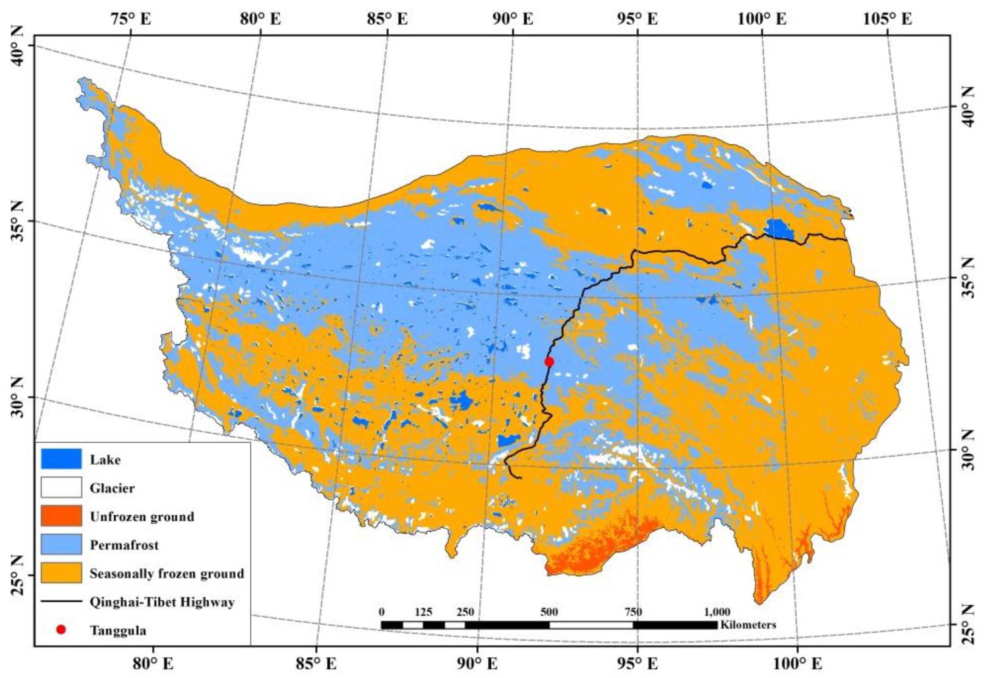
The data used herein were collected at the Tanggula observation station (TGL), which is located southwest of the Tanggula Mountain on the hinterland of the QTP (33.07° N, 91.93° E, Figure 1). It is the highest-altitude observation station in the permafrost region (5100 m a.s.l.) [55]. This monitoring site is located in the typical continuous permafrost zone with a vegetation type of alpine meadows (vegetation height is <10 cm, and vegetation cover is approximately 20–30%) [56]. The active layer thickness is approximately 3.15 m [56]. The previously reported soil texture data [57] were used herein. The mean annual air temperature was −4.4 °C and −5.8 °C in 2007 and 2008, respectively. The annual precipitation was 389 and 373 mm in 2007 and 2008, respectively, 80% of which was contributed by the precipitation between May and September. The atmospheric forcing data for Noah-MP included surface air temperature, specific humidity, wind speed, pressure, precipitation, downward shortwave and longwave radiation [58], measured from 1 August 2007 to 31 August 2008, with a 1 h temporal resolution. A four-component net radiometer (CM3, Kipp & Zonen, Delft, Holland) was used to measure four-component radiation at a height of 2.0 m above the ground [36]. The surface air temperature and specific humidity (HMP45C, Vaisala, Vantaa, Finland), wind speed (05103_L/RM, Campbell, CA, USA), and pressure were measured at three levels (2.0, 5.0, and 10.0 m) [36]. Precipitation was monitored using the Geonor T-200B all-weather precipitation gauge [36]. All meteorological data were recorded every 30 min automatically by CR3000 data loggers (Campbell Scientific, Logan, UT, USA) [36].
In addition, the daily soil temperature and moisture at various soil depths during the same period were used to verify the hydrothermal model performance of Noah-MP within the active layer. The soil temperature profile was measured at 14 depths (0.02, 0.05, 0.10, 0.20, 0.50, 0.70, 0.90, 1.05, 1.40, 1.75, 2.10, 2.45, 2.80, and 3.00 m) using a 105T/109 thermocouple probe (Campbell Scientific, Inc., Logan, UT, USA) with an accuracy of 0.1 °C/0.2 °C [36]. A Stevens hydroprobe (Stevens Water Monitoring System, Inc., Portland, ON, USA) with ± 3% accuracy [36] was used to obtain the soil moisture profile at 13 depths (0.05, 0.10, 0.20, 0.35, 0.50, 0.70, 1.05, 1.40, 1.75, 2.10, 2.45, 2.80, and 3.00 m). The soil temperature and moisture were measured at different soil depths, and these two variables were defined at four soil layers (0–10, 10–40, 40–100, and 100–200 cm with a depth of 2.00 m) in Noah-MP [58,59]; thus, the simulated and observed variables could not be directly compared. Linear interpolation was therefore applied to convert the field measurement into four soil layers [60], which inevitably increased the observation uncertainty and relative error between the simulated and observed values.
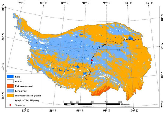
Figure 1.
Location of the Tanggula observation station on the QTP. The permafrost map [6], distribution of lakes [61] and glaciers [62] were obtained from previous studies.
Figure 1.
Location of the Tanggula observation station on the QTP. The permafrost map [6], distribution of lakes [61] and glaciers [62] were obtained from previous studies.
2.2. Noah-MP Numerical Experiments
2.2.1. Model Description
Noah-MP has been augmented in different physical processes with recent improvements in land surface models (LSMs) [51,52,63,64,65,66]. Compared with most traditional LSMs, Noah-MP has a significant advantage because of its incorporation of different parameterization schemes for several key physical processes within a unified dynamic framework [42,51,52,67]. This facilitates the implementation of an ensemble simulation, making Noah-MP a feasible LSM for investigating the uncertainty of ensemble simulation and sensitivity of physical process [42,68,69,70,71,72,73,74,75,76]. Many physical processes were incorporated into 2–5 parameterization schemes to select [51]. The initial conditions considerably impacted the outputs of LSMs [77]; therefore, to eliminate the anomalies arising from the initial state, it is imperative for the predicted variables to reach an equilibrium state for which spin-up is required [53]. Spin-up is the time taken by an LSM to reach a state of statistical equilibrium under a given atmospheric forcing [78,79]. Noah-MP requires a long time to reach equilibrium for the soil hydrothermal regime before it can be used for initialization [80,81]. Therefore, the atmospheric forcing data for 1 year before the study period were used herein to iteratively drive Noah-MP until the soil hydrothermal regime reached equilibrium, which would be satisfied when the simulation difference between the predicted variables for two consecutive years is <0.1% of the annual mean [80,81]. It is noteworthy that the soil depth simulated by Noah-MP is only 2 m [58,59], whereas the thickness of the active layer at the TGL station is 3.15 m [56]. Therefore, the simulation results only reflect the soil hydrothermal dynamics within the partial active layer.
2.2.2. Noah-MP Default Parameterization Scheme and Ensemble Numerical Experiment
The parameterization schemes for 11 physical processes controlling the hydrothermal regime within the active layer were selected in this study (Table 1). Parameterization schemes for these physical processes were randomly combined, and a total of 23,040 possible combinations were obtained (Supplementary Materials). Then, ensemble simulations and sensitivity tests were conducted. Among these combinations, the default combination of schemes (Def) was of particular importance, as recommended by Niu et al. (2011) [51], and was most commonly adopted in land surface modeling. Herein, Def was employed to test the validity of the atmospheric forcing data and the applicability of the model in hydrothermal simulation (Table 2). The first ensemble experiment comprising 23,040 members (Ens1, Table 2) was designed to analyze the uncertainty in ensemble simulation. Based on the analysis results of the previous step, additional Noah-MP ensemble simulations (Ens2 and Ens3, Table 2) were conducted, with configurations consistent with Ens1, except for frozen soil permeability (INF). Finally, two optimal experiments (Opt1 and Opt2, Table 2) were designed to compare the disparity in model performance between two optimal combinations of parameterization schemes obtained from the TOPSIS, in which INF-1 (NY06) and INF-2 (Koren99) were used in turn.

Table 1.
Noah-MP physical processes and their parameterization schemes used in this study.
Table 1.
Noah-MP physical processes and their parameterization schemes used in this study.
| Physical Process | Parameterization Scheme |
|---|---|
| Soil moisture threshold for plant transpiration (BTR) | 1: Noah type [65] [Default] as a function of soil moisture 2: Community Land Model (CLM) type [82], matric potential related 3: Simplified Biosphere Model (SSiB) type [83], matric potential related |
| Surface-layer exchange coefficient (SFC) | 1: Monin–Obukhov (M-O) [84] [Default], M-O similarity theory 2: Noah type [64], neglecting the zero-displacement height |
| Supercooled liquid water in frozen soil (FRZ) | 1: NY06 [85] [Default], no iteration, general form of the freezing-point depression equation 2: Koren99 [86], Koren’s iteration, variant freezing point depression |
| Frozen soil permeability (INF) | 1: NY06 [85] [Default], linear effect, more permeable, as a function of soil moisture and ice 2: Koren99 [86], nonlinear effect, less permeable, function of liquid water |
| Radiation transfer (RAD) | 1: Modified two-stream [87], canopy gaps from 3D structure and solar zenith angle 2: Two-stream applied to a grid cell [87], no canopy gap 3: Two-stream applied to a vegetated fraction [87] [Default], gaps from the vegetated fraction (gap = 1−FVEG) |
| Snow surface albedo (ALB) | 1: BATS [88], computes snow surface albedo for direct and diffuse radiation over visible and near-infrared wave bands 2: CLASS [89] [Default], computes the overall snow surface albedo accounting for fresh snow albedo and snow age |
| Partitioning precipitation into rainfall and snowfall (PCP) | 1: Jordan [90] [Default], relatively complex functional form 2: BATS, assumes all precipitation as snowfall when air temperature below freezing temperature plus 2 °C 3: Assumes all precipitation as snowfall when air temperature below the freezing temperature 4: Wet-bulb temperature-based [91], a snow-rain partitioning scheme using the wet-bulb temperature (Tw), which is closer to the surface temperature of a falling hydrometeor than surface air temperature (Ta) and would lead to a larger fraction of snowfall |
| Lower boundary of soil temperature (TBOT) | 1: Zero-flux scheme, zero heat flux from the bottom soil layer 2: Noah [Default], TBOT at 8 m soil depth, read from a preset file |
| The first-layer snow or soil temperature time scheme (TEMP) | 1: Semi-implicit [Default], flux top boundary condition 2: Fully implicit, temperature top boundary condition |
| Surface resistance to evaporation (SRES) | 1: Sakaguchi and Zeng’s scheme [92] [Default] 2: Sellers’s scheme [93] |
| Runoff and groundwater (RUN) | 1: TOPMODEL with an equilibrium water table [94] 2: Original surface and subsurface runoff (free drainage) [95] [Default] 3: BATS surface and subsurface runoff (free drainage) [70,96,97] 4: Variable infiltration capacity model surface runoff scheme [98] 5: Dynamic VIC surface runoff scheme [99] with the Philip infiltration scheme |
Table 2.
Setup of the numerical experiments.
Table 2.
Setup of the numerical experiments.
| Experiment Name | Description of Experiment | Members |
|---|---|---|
| Def | In situ observation as the forcing data, default combination of parameterization schemes | 1 |
| Ens1 | Forcing data are the same as those used in Def, parameterization schemes for all 11 physical processes were combined | 23,040 |
| Ens2 | Forcing data are the same as those used in Def, INF = 1, parameterization schemes for the other 10 physical processes were combined | 11,520 |
| Ens3 | Forcing data are the same as those used in Def, INF = 2, parameterization schemes for the other 10 physical processes were combined | 11,520 |
| Opt1 | Forcing data are the same as those used in Def, INF = 1, configurations of optimal parameterization scheme for the other 10 physical processes were obtained based on the TOPSIS | 1 |
| Opt2 | Forcing data are the same as those used in Def, INF = 2, configurations of optimal parameterization scheme for the other 10 physical processes were obtained based on the TOPSIS | 1 |
2.3. Evaluation and Analysis Methods
Soil temperature and moisture were considered as the simulated variables. The daily corresponding moments of simulation and observation were used for evaluating the simulation accuracy, and the root mean square error (RMSE), mean bias error (MBE), and correlation coefficient (R) between simulated and observed variables were used as evaluation indexes. Herein, the uncertainty of the ensemble simulation was evaluated and the sensitivity of multiple parameterization schemes in Noah-MP were analyzed using Natural Selection and Tukey’s test, and RMSE was used in both methods to evaluate the model performance. Furthermore, TOPSIS was used to identify the optimal combination of parameterization schemes for improving the overall simulation accuracy of hydrothermal processes within the active layer. The evaluation and analysis methods used herein were described in subsequent sections.
2.3.1. Model Evaluation
The model performance in the simulation of soil temperature and moisture within the active layer was quantified using RMSE, MBE, and R as follows:
where and were the simulated and observed values, respectively, and were the averages of the simulated and observed values, respectively, and was the number of observations.
2.3.2. Natural Selection
First, the RMSE of each parameterization scheme combination was determined in Ens1. For each physical process, the simulation results of all scheme combinations were regarded as the statistical population [42,54], so the statistical population of each physical process was identical. The RMSE were ranked in ascending order, and the samples with RMSEs below the 5th percentile and above the 95th percentile were extracted from Ens1. The samples with RMSEs below the 5th percentile were classified as the best membership (1152 members), because their model performance was better compared with samples with RMSEs above the 95th percentile, while the latter were classified as the worst membership (1152 members). The frequency with which a given parameterization scheme was employed in each physical process among the best and worst membership was determined. For a given physical process, if a specific parameterization scheme was selected more among the best membership, the model accuracy was high. Contrarily, if the scheme was selected more among the worst membership, the model accuracy was considered low. Thus, Natural Selection could be used to determine the applicability of the parameterization scheme in a given physical process.
2.3.3. Tukey’s Test
Tukey’s test [100,101] was used to evaluate the difference in model performance for different parameterization schemes in a given physical process. For example, the radiation transfer physical process (RAD) had three parameterization schemes, with , , and as the scheme means, and a statistical hypothesis test was used to compare each pair of population means and for all where the null and alternative hypotheses were as follows:
Tukey’s test used the studentized range distribution:
where was the mean square error of all samples for two schemes, was the total sample size for all schemes (for all three radiation schemes in RAD was 23,040), was the number of parameterization schemes ( for RAD), was the scheme means, and were the sample sizes for the ith and jth parameterization schemes, respectively, was the sum of the square error, was the maximum of the two parameterization scheme means being compared, was their minimum, and was the degree of freedom associated with . Based on Tukey’s test, it could be inferred that two population means exhibited a significant disparity if
where was the significance level (set to 0.05) and could be obtained by consulting the table of the studentized range distribution [42,54]. If the value of , made Equation (8) true, then the null hypothesis should be rejected at the significance level of 0.05; otherwise, the null hypothesis should be accepted at a 95% confidence level.
2.3.4. TOPSIS
As a common multi-criteria decision-making technique, Technique for Order of Preference by Similarity to Ideal Solution (TOPSIS) is a practical and useful method for ranking and selecting a number of possible alternatives by measuring Euclidean distances, which was previously presented by Chen [102] and used to determine a solution with the shortest distance to the positive-ideal solution and the farthest distance from the negative-ideal solution [103]. TOPSIS has been applied in several studies, such as ranking general circulation models [104,105,106] and identifying the best physical parameterization schemes in WRF [107,108,109]. This method was applied to identify the best scheme among the sensitivity experiments in which the simulated variable for each soil layer was utilized as criteria. For example, the RAD physical process had three parameterization schemes and the Noah-MP estimated temperature and moisture at four soil layers; thus, three alternatives and four decision-making criteria could be used. For the ith (i = 1, 2, 3) parameterization scheme in the RAD physical process, the criteria of the jth (j = 1, 2, 3, 4) soil layer was denoted as , which referred to the RMSE of temperature or moisture at the jth soil layer simulated by the ith parameterization scheme. The steps for applying the TOPSIS were briefly described as follows:
(1) An evaluation matrix comprising three alternatives and four criteria was created with the intersection of each alternative and criteria given as ; therefore, we had a matrix .
(2) The normalized decision matrix was calculated. The matrix was then normalized to form the matrix using the normalization method:
(3) The positive-ideal and negative-ideal solutions were determined. Here, the positive-ideal solution () and negative-ideal solution () referred to the minimum and maximum of the RMSE, respectively, for the ith parameterization scheme.
(4) The separation measures were calculated using the two-dimensional Euclidean distance. The separation of the ith parameterization scheme from the positive-ideal solution was given as
Similarly, the separation from the negative-ideal solution was given as
(5) The relative closeness to the ideal solution was calculated. The relative closeness of the ith parameterization scheme with respect to and was defined as
where if and only if the alternative solution had the best condition, and if and only if the alternative solution had the worst condition.
(6) The alternatives were ranked according to .
3. Results
3.1. Simulation of Hydrothermal Process Within the Active Layer
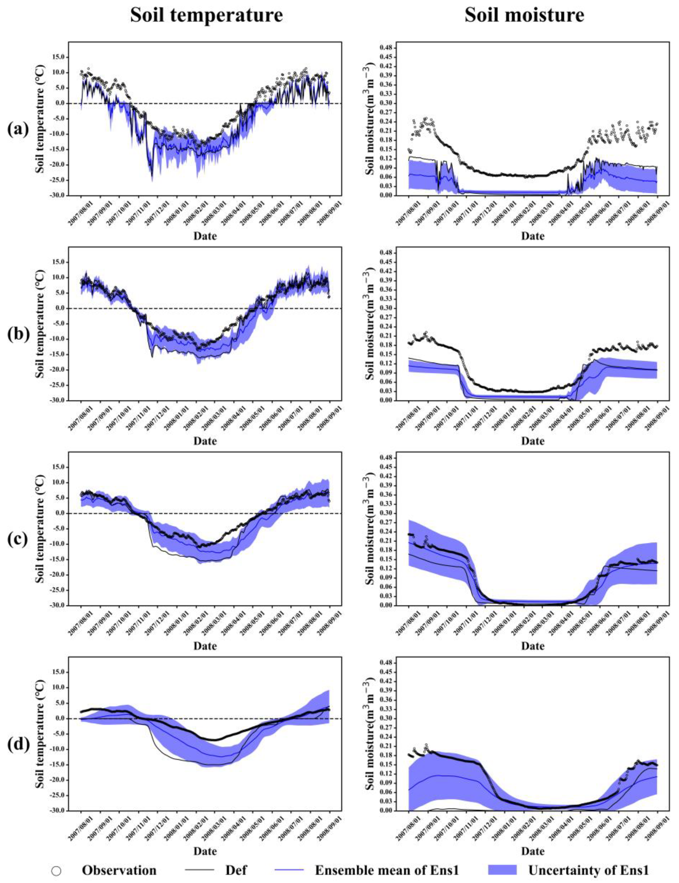
Noah-MP was used to estimate the soil temperature and moisture at four soil layers, i.e., 0–10, 10–40, 40–100, and 100–200 cm with a soil depth of 2.00 m [58,59]. The simulated soil temperature and moisture were compared with those obtained from field observation to evaluate the model performance. Figure 2 shows a comparison of the observed and simulated daily mean temperature and moisture of four soil layers at the TGL. Table 3 and Table 4 show the statistics of soil temperature and moisture at each soil layer for different numerical experiments, respectively. The soil temperature and moisture simulated by Noah-MP agreed well with those from observation. The freeze–thaw cycle could be well determined based on these two predicted variables in all experiments (for complete freeze–thaw cycle, R was > 0.9 in most cases).
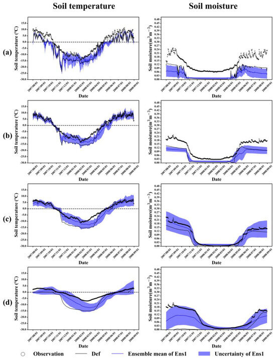
Figure 2.
Comparison of the observed and simulated soil temperature and moisture by Def and Ens1 for each soil layer from 1 August 2007 to 31 August 2008: topsoil (a), second layer (b), third layer (c), and bottom layer (d). The black hollow dots showed the observed values, the black curve was the time series simulated by Def, the blue curve was the ensemble mean of Ens1, and the uncertainty (blue shading) was one standard deviation of Ens1.
Table 3.
Root mean square error (RMSE), mean bias error (MBE), and correlation coefficient (R) of the simulated and measured soil temperature at four soil layers obtained via numerical experiments listed in Table 2 during complete freeze–thaw cycle, thawed period and frozen period.
Table 4.
Same as Table 3 but for soil moisture.
3.1.1. Validation of Soil Temperature
Soil temperature simulated by Def was generally close to the observed values but was underestimated for each soil layer during a complete freeze–thaw cycle. Furthermore, Ens1 showed a significant improvement compared with Def for all soil layers, which was consistent with the finding that the overall multi-model averaging yielded better results than that of any single model [60,110]. Def performed better during the thawed period than that during the frozen period in the soil temperature simulation, which was possibly due to the release of latent heat during the frozen period [56] that could not be accurately described by the LSM. Meanwhile, Ens1 also performed better during the frozen period than that during the thawed period. Notably, the uncertainty of Ens1 and the accuracy of its ensemble mean showed similar temporal patterns with high uncertainty during the frozen period and low uncertainty during the thawed period. The ensemble simulation could yield better simulation accuracy; however, the excessive computational costs limited its applicability.
3.1.2. Validation of Soil Moisture
Def simulated soil temperature better than soil moisture; however, it could capture the seasonal dynamic of soil moisture except for the bottom layer during a complete freeze–thaw cycle. Figure 2 showed that Def underestimated the soil moisture for four soil layers with the first and bottom layer showing a more significant underestimation. Combining RMSE, MBE, and R showed that the performance of Def at the bottom layer was the worst. Different from the soil temperature simulation, the underestimation of soil moisture during the thawed period was more remarkable than that during the frozen period, which was probably because the soil moisture during the thawed period was controlled by several factors, such as the thawing of soil [56,111], precipitation infiltration [56,111], soil evaporation [43,59], capillary force [56], vegetation transpiration [112], etc., and the model descriptions for the combined effects of these factors were also not satisfactory.
Compared with Def, Ens1 considerably improved the underestimation of soil moisture during the frozen period: the average RMSE decreased from 0.048 to 0.032 m3/m3, MBE increased from −0.038 to −0.025 m3/m3, and R increased from 0.578 to 0.890 for all soil layers (Table 4). During the thawed period, Ens1 improved the soil moisture simulation at the third and fourth layer, whereas the model performance deteriorated for soil moisture at the first and second layer. This proved that Def performed considerably better than the other scheme combinations in soil moisture simulation for shallow layers. The uncertainty in soil moisture simulated by Ens1 was higher during the thawed period and lower during the frozen period, which was mainly because it was influenced by more factors during the thawed period.
3.2. Results of Natural Selection
The RMSE values for the soil temperature and moisture of 23,040 scheme combinations in 11 physical processes were determined and ranked in ascending order for all soil layers. The samples below the 5th percentile of the RMSE were classified as the best membership and those above the 95th percentile were classified as the worst membership, and the selected frequency of each scheme was categorized into these two groups. The subfigures above and below the horizontal axis in Figure 3 show the selected frequency of each parameterization scheme among the best and worst membership, respectively.
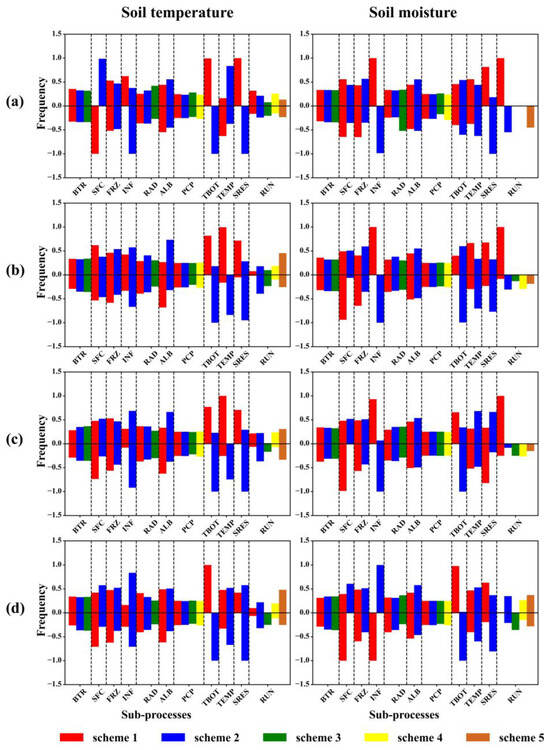
Figure 3.
Selected frequency of different parameterization schemes in each physical process for the simulation of soil temperature and moisture for each soil layer: topsoil (a), second layer (b), third layer (c), and bottom layer (d), respectively, in the best membership (0–1) and worst membership (−1–0) in Ens1.
Considering the ALB for soil temperature at the top soil layer as an example, the selected frequencies of the ALB scheme 1 (ALB-1) and scheme 2 (ALB-2) among the best membership were 0.44 and 0.56, respectively, indicating 44% combinations of schemes for 1152 samples using ALB-1 and 56% combinations of schemes using ALB-2 for the best membership. The difference in the selected frequency among the best membership implied that ALB-2 would yield more favorable simulation results than ALB-1. For the remaining soil layers, the selected frequency of ALB-1 and ALB-2 among the best and worst membership was consistent with the top soil layer, which implied that the soil temperature simulation was sensitive to ALB at four soil layers. The soil temperature simulation for topsoil was sensitive to INF, and INF-1 was more preferable. However, the selected frequency of INF-1 and INF-2 for the other three soil layers showed that the soil temperature simulation was insensitive to INF, because the frequency of these two schemes was very close among the best membership and worst membership. There was no significant difference in the selected frequency of schemes for BTR, FRZ, RAD, PCP, and RUN for most soil layers (Figure 3), implying that the soil temperature simulation was also insensitive to these physical processes. Notably, significant differences were observed between the selected frequency of the parameterization schemes for SFC, ALB, TEMP, and SRES for most soil layers, and the difference in the selected frequency for TBOT was particularly significant for four soil layers. The sensitivity of physical processes in the soil moisture simulation differed from that of soil temperature. The selected frequency of the parameterization schemes for FRZ, INF, and RUN differed considerably in the soil moisture simulation. Thus, the uncertainty of parameterization schemes for these physical processes were significant. In other words, the sensitivity of the Noah-MP ensemble simulation to these processes in the soil moisture simulation was observed for most soil layers.
3.3. Results of Tukey’s Test
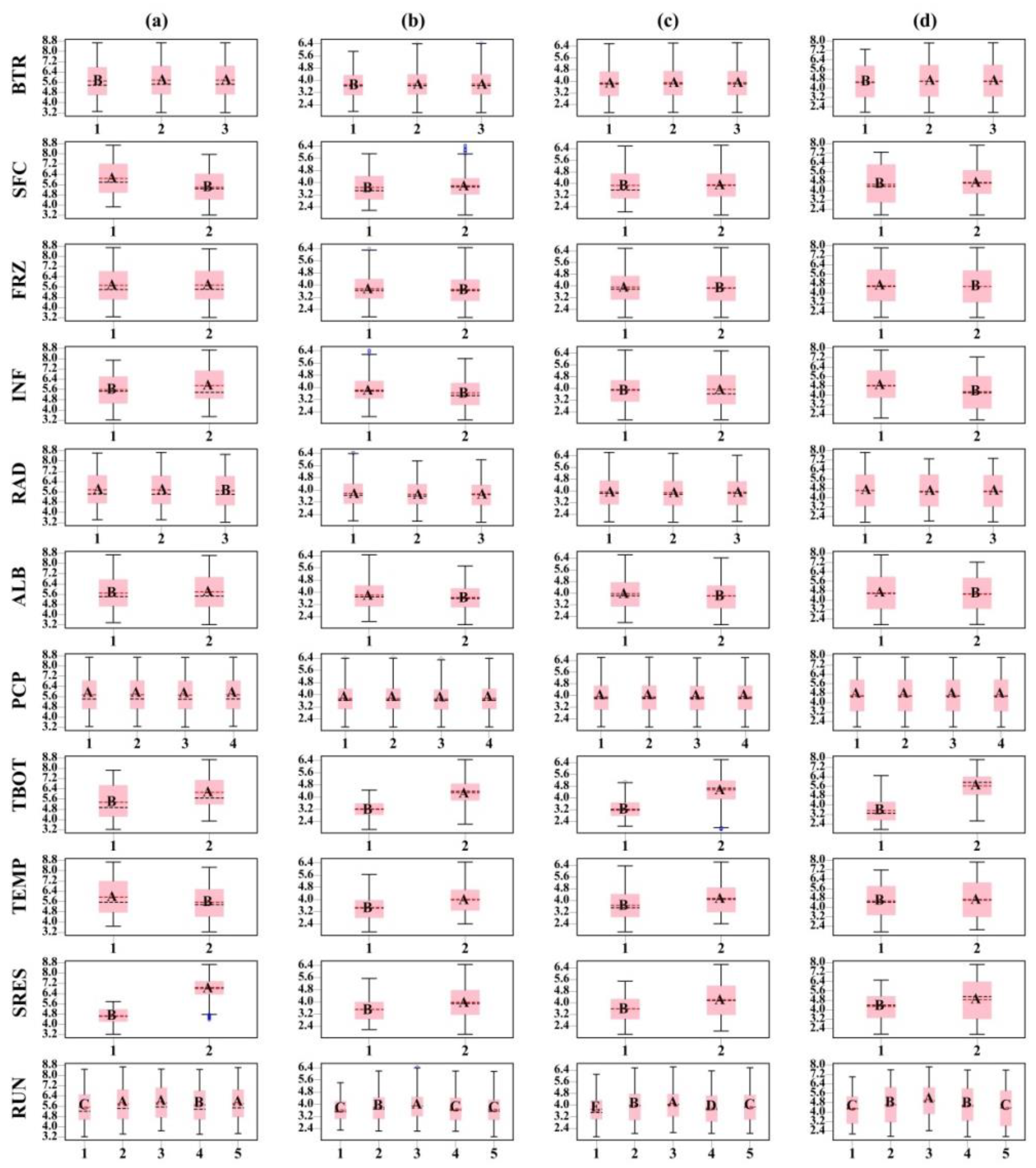
The uncertainty of the parameterization schemes in each physical process was analyzed by adopting Tukey’s test. Figure 4 and Figure 5 showed the analysis results for the RMSE of soil temperature and moisture in Ens1, respectively. First, the RMSE of each combination of parameterization schemes in Ens1 was calculated, obtaining a total number of 23,040 for both soil temperature and moisture. For Ens1, all 23,040 RMSEs were independent of each other. Before performing Tukey’s test, the assumptions of normality and equality of variances were checked. If the raw RMSE deviated substantially from normality, they were log-transformed. For example, the physical process of RAD had three parameterization schemes; thus, each scheme corresponded to 7680 RMSEs. In both Figure 4 and Figure 5, there was a significant difference between the parameterization schemes that did not share a letter at the 95% confidence level, and the parameterization scheme with the letter “B” was superior to that with the letter “A” because its mean RMSE value was much smaller. Similarly, the scheme with the letter “C” outperformed that with the letter “B”. Therefore, the smaller the average value of RMSE, the better the model performance of the scheme. Within the framework of Tukey’s test, whether the hydrothermal simulation was sensitive to a given physical process depended on the statistical significance of the difference among the parameterization schemes. In other words, a physical process could be considered insensitive when all of its schemes shared a single letter, and it could be considered sensitive when any two schemes were assigned different letters. For example, TBOT-1 and TBOT-2 were labeled with the letters “B” and “A” sequentially in the soil temperature simulation for four soil layers, where the average RMSE of TBOT-1 was smaller than that of TBOT-2. This implied that the difference between TBOT-1 and TBOT-2 was significant and consistent across all soil layers, and TBOT-1 was more likely to produce more preferable simulation results than TBOT-2 for soil temperature, which was consistent with the results from Natural Selection. Similarly, the significant and consistent difference between the parameterization schemes for SFC, ALB, TEMP, and SRES in the soil temperature simulation was observed for most soil layers, which also corresponded with the results from Natural Selection. According to results of Tukey’s Test for soil temperature, FRZ showed a consistent sensitivity at most soil layers and FRZ-2 outperformed FRZ-1, which could not be identified by Natural Selection. This indicated that compared with Natural Selection, more preferable parameterization schemes could be accurately and comprehensively identified by Tukey’s test. The main reason was that Natural Selection only considered the best and worst membership (sample size was about 1152), accounting for only a very small fraction (5%) of the total simulation results, while Tukey’s test considered all 23,040 samples.
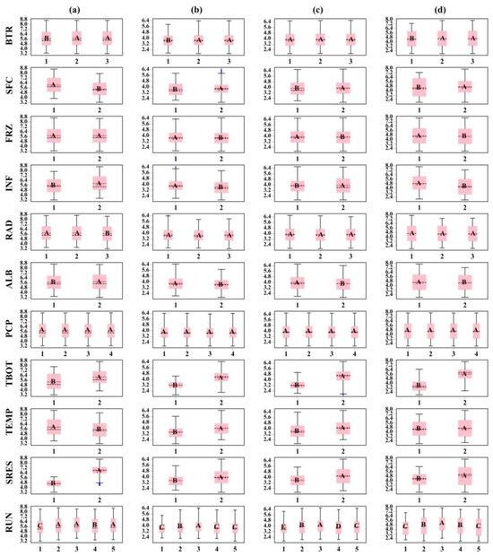
Figure 4.
Tukey’s boxplot for the RMSE of soil temperature at four layers: (a) topsoil, (b) second layer, (c) third layer, and (d) bottom layer. For simulation at each soil layer, the subfigures from top to bottom show the results for 11 physical processes. The ends of the boxes represent Q1 (25th percentile) and Q3 (75th percentile). The whiskers indicate the upper and lower bound, where Q3 + 1.5 × IQR represent the upper bound and Q1 − 1.5 × IQR represent the lower bound, and IQR (Interquartile Range) = Q3 − Q1. The horizontal black and red lines indicate the mean and median (50th percentile), respectively. The outliers are shown as blue circles. For each subfigure, the letters represent different classification of corresponding parameterization schemes; at the 95% confidence level, the schemes in the same physical process that did not share a letter were significantly different.
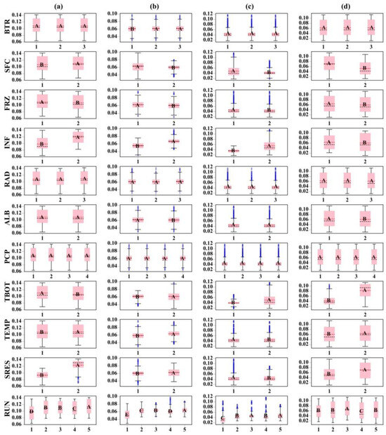
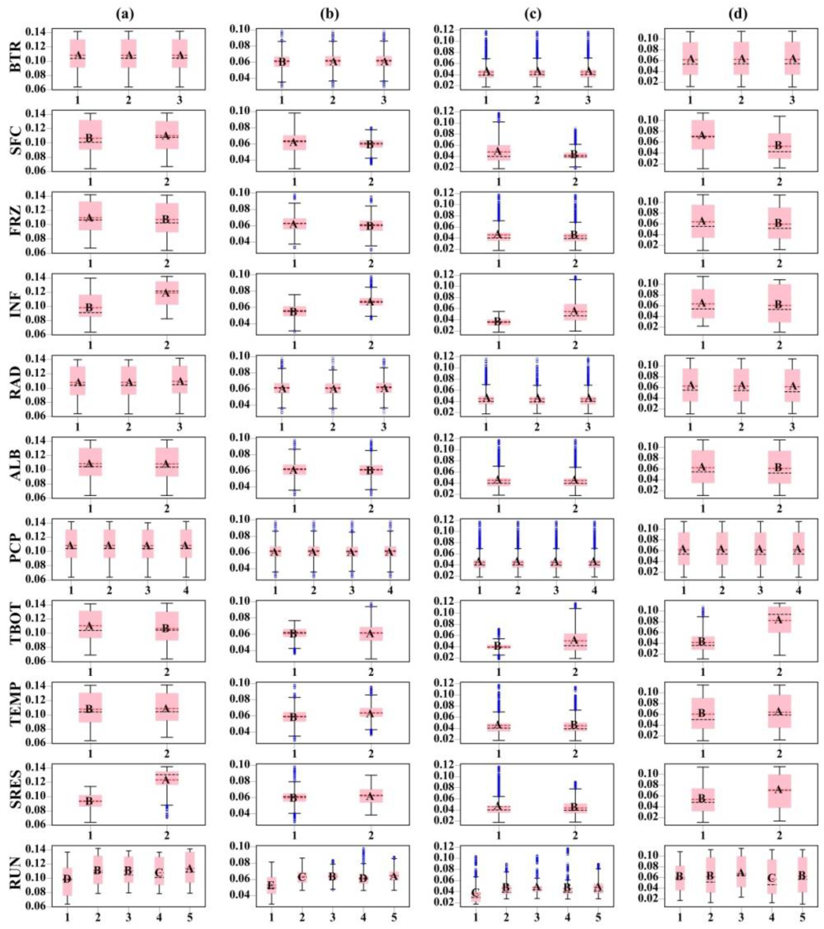
Figure 5.
Tukey’s boxplot for the RMSE of soil moisture at four layers: (a) topsoil, (b) second layer, (c) third layer, and (d) bottom layer. For simulation at each soil layer, the subfigures from top to bottom show the results for 11 physical processes. The ends of the boxes represent Q1 (25th percentile) and Q3 (75th percentile). The whiskers indicate the upper and lower bound, where Q3 − 1.5 × IQR represent the upper bound and Q1 − 1.5 × IQR represent the lower bound, and IQR (Interquartile Range) = Q3 − Q1. The horizontal black and red lines indicate the mean and median (50th percentile), respectively. The outliers are shown as blue circles. For each subfigure, the letters represent different classification of corresponding parameterization schemes; at the 95% confidence level, the schemes in the same physical process that did not share a letter were significantly different.
For both soil temperature and moisture, RUN showed consistent sensitivity across all soil layers, which indicated that RUN-1 yielded more favorable simulation results in Ens1 than the other four parameterization schemes. FRZ, TBOT, and SRES exhibited similar model performance for both temperature and moisture at most soil layers. In addition, the performances of TEMP and INF were consistent for both predicted variables for some soil layers. Generally speaking, the results of Tukey’s test for sensitivity to physical processes were consistent with the results of Natural Selection. Tukey’s test identified more parameterization schemes with almost similar model performance for soil temperature and moisture. This would facilitate the establishment of an optimal combination of existing parameterization schemes, which could produce more favorable simulations of soil temperature and moisture simultaneously.
3.4. Ranking of Model Performance for Each Parameterization Scheme
In the previous sections, Natural Selection and Tukey’s test were used to analyze the uncertainty of parameterization schemes in each physical process. It was found that the uncertainty analysis was useful to identify sensitive physical processes and preferable parameterization schemes. The model performance of some parameterization schemes in the simulation of soil temperature and moisture was consistent at most soil layers, which provided useful guidance for determining an optimal scheme combination that could overall improve the hydrothermal simulation. TOPSIS was adopted to predict the effects of different parameterization schemes on soil temperature and moisture for four soil layers and evaluate the model performance of each scheme in key physical processes. This method also allowed ranking alternatives [113], making it easier to choose the optimal parameterization scheme. Taking each simulated variable for four soil layers as the objective for simultaneous optimization, an optimal scheme combination was identified to improve the model performance of Noah-MP in the simulation of soil temperature and moisture simultaneously. Choosing different parameterization schemes in physical processes could lead to a significant change in its ranking [114], and the ranking of performance scores would describe the divergence among different parameterization schemes in each physical process [114].
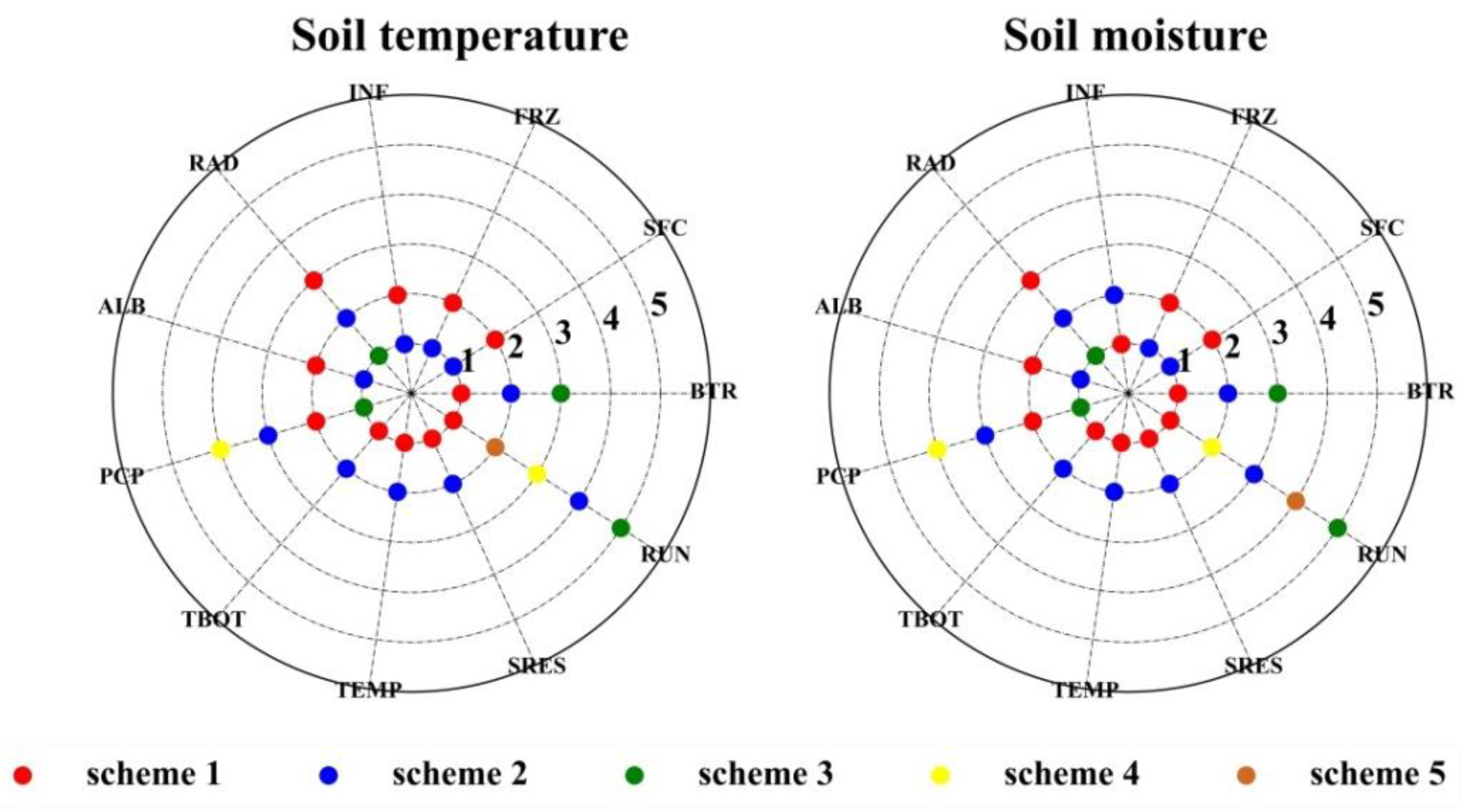
The evaluation of parameterization schemes in 11 physical processes using TOPSIS (Figure 6) showed that the ranking of parameterization schemes was consistent for the simulation of soil temperature and moisture in most physical processes. For physical process of BTR, BTR-1 was the best scheme followed by BTR-2, and BTR-3 proved to be the worst one, which was consistent in the simulation of both soil temperature and moisture. Moreover, the ranking of the parameterization schemes in SFC, FRZ, RAD, ALB, PCP, TBOT, TEMP, and SRES was identical for both simulated variables, which indicated that the model performance of each scheme for most physical processes were consistent in both variables and confirmed a strong interaction between thermal and hydrological dynamics of the active layer soil [115]. Although the ranking of each parameterization scheme of the RUN was different for the two predicted variables, their optimal scheme was the same. For the INF process, the optimal schemes for soil temperature and moisture were conflicting and needed further evaluation.
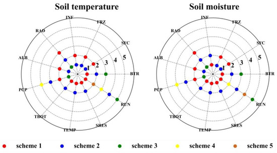
Figure 6.
Plot of performance scores determined based on TOPSIS used to evaluate the overall model performance of parameterization schemes in each physical process for hydrothermal simulation at four soil layers. Each dot in the radar chart corresponds to a parameterization scheme for 11 physical processes, distinguished by various colors. The placement of these dots in the chart reflects the comparative performance of each scheme, where the dots closer to the center imply that the corresponding scheme may be more favorable, and the numbers (1, 2, 3, 4, and 5) inditate the degree of significance.
4. Discussion
During the frozen period, Opt1 and Opt2 showed the best model performance for RMSE and MBE in soil moisture simulation at shallow layers among all numerical experiments (Table 4), and Opt2 outperformed Opt1 (for R at four layers and RMSE and MBE at deep layers). Figure 7 also indicates that the uncertainty of both Ens2 and Ens3 was significantly reduced compared with the thawed period (with the smaller uncertainty in Ens3), which suggested that in terms of the primary function of INF, both parameterization schemes could substantially counteract the disturbance of other physical processes to soil moisture simulation, and INF-2 was more favorable. Controlled by the soil moisture simulation during the same period, the soil temperatures simulated by Opt1 and Opt2 both agreed better with observation than Def, wherein both RMSE and MBE were significantly improved and only R was slightly deteriorated (Table 3). Comparison of the simulation results of Opt1 and Opt2 showed that Opt2 would generally yield better results for soil temperature during the frozen period (Table 3).
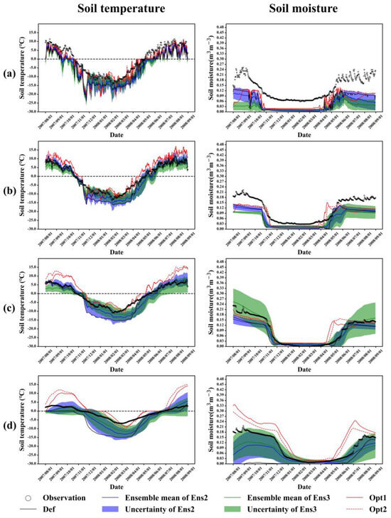
Figure 7.
Comparison of the observed and simulated soil temperature and moisture by Def, Ens2, Ens3, Opt1, and Opt2 for each soil layer from 1 August 2007 to 31 August 2008: topsoil (a), second layer (b), third layer (c), and bottom layer (d). Black hollow dot: observation, black curve: time series simulated by Def, blue curve: ensemble mean of Ens2, blue shading: uncertainty is one standard deviation of Ens2, green curve: ensemble mean of Ens3, green shading: uncertainty is one standard deviation of Ens3, red solid line: time series simulated by Opt1, red dashed line: time series simulated by Opt2.
Even if the parameterization schemes for the other 10 processes were configured identically, different parameterization schemes of INF would produce widely divergent simulation results in the soil moisture simulation during the thawed period, which was consistent with the findings of Hu [53]. This might reflect the response of soil moisture during the thawed period to the thawing process, because these two schemes had the same permeability at the soil layer without ice [53]. Compared with the ensemble means of Ens1, Ens2, and Ens3, Def matched better with the observation in the simulation of soil temperature and moisture during the thawed period, which indicated that Def had an advantage over a considerable number of scheme combinations in the hydrothermal simulation during the same period. However, compared with Def, Opt1 and Opt2 showed better model performance for soil moisture during the thawed period, and a comprehensive comparison of three statistical indicators (Table 4) indicated that Opt2 showed the best agreement with the observation. Moreover, Opt1 and Opt2 showed better model performance for RMSE and MBE in soil temperature at the top layer among all numerical experiments, and Opt2 was more superior. Although, compared with Def, neither Opt1 nor Opt2 could improve the soil temperature simulation for the deeper three layers during the thawed period and even led to a deterioration, Opt2 significantly improved the R (R increased from 0.50 to 0.71, Table 3) at the bottom layer during the same period.
For the hydrothermal simulation within the active layer, the improvement of Opt1 and Opt2 during the frozen period was more significant than that during the thawed period, and the improvement for soil moisture was more significant than that for soil temperature; in other words, any configuration for a combination of parameterization schemes had difficulty in simulating each variable well, and the optimal scheme combination might vary with time (between the thawed period and frozen period), and the accuracy of the soil moisture simulation could be improved using an optimal combination of parameterization schemes but at the expense of the simulation accuracy of soil temperature. To address this issue, further investigation was required to understand the characteristics of detailed parameters for the thermal dynamics within the active layer in this region, and adopting a more detailed parameterization of the thermal properties for enhancing the heat transfer would be one of the most promising approaches to enhancing the performance of Noah-MP in the soil temperature simulation.
5. Conclusions
Herein, based on the observation of hydrothermal regime within the active layer from 1 August 2007 to 31 August 2008 at TGL, the variations in soil temperature and moisture during a complete freeze–thaw cycle were simulated using Noah-MP to test the fitting of the scheme combinations with observation. By conducting an ensemble simulation with 23,040 scheme combinations for 11 physical processes, the feasibility of the model for hydrothermal simulation within the active layer was first determined. Then, the sensitivity of parameterization schemes for soil temperature and moisture were explored using Natural Selection and Tukey’s test. Finally, TOPSIS was used to identify the optimal combination of parameterization schemes that could overall improve the hydrothermal simulation within the active layer. The main findings of this study are as follows:
- Def could well reflect the seasonal pattern of hydrothermal dynamics within the active layer with a systematic underestimation. Compared with Def, Ens1 considerably improved the hydrothermal simulation during the frozen period, which was very limited or even negative for shallow soil during the thawed period. The large uncertainty of Ens1 in the soil temperature simulation during the frozen period and soil moisture simulation during the thawed period was mainly caused by their respective complex influencing factors.
- The results of Natural Selection revealed that for most soil layers, the selected frequency of parameterization schemes in SFC, ALB, TEMP, TBOT, and SRES was consistent in soil temperature simulation and that the selected frequency for FRZ, INF, and RUN was consistent for soil moisture. The results of Tukey’s test generally agreed with the results from Natural Selection, and Tukey’s test identified more parameterization schemes with similar model performance for both soil temperature and moisture. Moreover, the results of TOPSIS showed that the determination of the optimal scheme was consistent for the simulation of soil temperature and moisture in each physical process except for INF.
- Both parameterization schemes in INF considerably reduced the uncertainty in soil moisture simulation during the frozen period. The soil moisture simulated by Opt1 and Opt2 at shallow layers during the frozen period agreed better with the observations compared with that of Def, and Opt2 yielded better simulation results than Opt1. Influenced by the thawing process, Opt1 and Opt2 showed better performance than Def in the soil moisture simulation during the thawed period, and Opt2 showed the best performance.
- Controlled by the soil moisture simulation during the frozen period, the soil temperature simulated by Opt1 and Opt2 agreed better with observation than Def during the same period, and Opt2 yielded better simulation accuracy. Compared with Def, Opt1 and Opt2 showed better performance for RMSE and MBE at the top layer in the soil temperature simulation during the thawed period, and Opt2 showed an overwhelming better performance for R at four soil layers compared with Opt1. Neither Opt1 nor Opt2 could improve the soil temperature simulation for the deeper three layers during the thawed period and even led to a deterioration, which indicated that Def had an advantage in the soil temperature simulation during the thawed period.
Supplementary Materials
The following are available online at https://www.mdpi.com/article/10.3390/land14020247/s1, The supplementary file contains the ensemble simulation results of Ens1 from 1 August 2007 to 31 August 2008, and also includes a data description document.
Author Contributions
Conceptualization, Y.J., R.L., T.W., X.W., S.W., G.H., X.Z., Y.X. and E.D.; Methodology, Y.J., R.L., T.W., X.W., S.W., J.Y., G.H., X.Z., J.S., Y.X., E.D. and Y.Q.; Software, Y.J., S.W., J.S. and Y.X.; Validation, Y.J., R.L., T.W., X.W., S.W., J.Y., G.H., X.Z., J.S., Y.X. and E.D.; Formal analysis, Y.J., R.L., S.W., J.Y., G.H., X.Z., J.S., Y.X., E.D. and Y.Q.; Investigation, Y.J., R.L., T.W., X.W., S.W., J.Y., G.H., X.Z., J.S., Y.X., E.D. and Y.Q.; Resources, Y.J. and S.W.; Data curation, Y.J., S.W., X.Z., J.S., E.D. and Y.Q.; Writing—original draft, Y.J., X.W., S.W., J.S., Y.X. and E.D.; Writing—review & editing, Y.J., R.L., T.W., X.W., S.W., J.Y., G.H., X.Z., E.D. and Y.Q.; Visualization, Y.J., Shen-ning Wang, J.Y., J.S., Y.X., E.D. and Y.Q.; Supervision, R.L., T.W., X.W., J.Y., G.H. and X.Z.; Project administration, R.L., T.W., X.W. and G.H.; Funding acquisition, R.L., T.W. and X.W. All authors have read and agreed to the published version of the manuscript.
Funding
This research was funded by the National Natural Science Foundation of China (W2412013, 42471168), National Key Research and Development Program of China (2020YFA0608502, 2023YFC3206300), National Natural Science Foundation of China (U23A2062, 42071093), Gansu Provincial Science and Technology Program (22ZD6FA005), the State Key Laboratory of Cryospheric Science (SKLCS-ZZ-2023), and the Natural Science Foundation of Gansu Province (22JR5RA061, 22JR5RA054).
Data Availability Statement
Some or all of the data generated or analyzed in this study and the code supporting the findings during this study are available from the corresponding author upon reasonable request. The corresponding author can share data with other researchers who send their request to this email address: liren@lzb.ac.cn.
Conflicts of Interest
The authors declare that they have no known competing financial interests or personal relationships that could have appeared to influence the reported work.
References
- Qiu, J. China: The third pole. Nature 2008, 454, 393–396. [Google Scholar] [CrossRef]
- Yao, T.; Bolch, T.; Chen, D.; Gao, J.; Immerzeel, W.; Piao, S.; Su, F.; Thompson, L.; Wada, Y.; Wang, L.; et al. The imbalance of the Asian water tower. Nat. Rev. Earth Environ. 2022, 3, 618–632. [Google Scholar] [CrossRef]
- Lei, J.; Shi, Z.; Xie, X.; Sha, Y.; Li, X.; Liu, X.; An, Z. Seasonal Variation of the Westerly Jet over Asia in the Last Glacial Maximum: Role of the Tibetan Plateau Heating. J. Clim. 2021, 34, 2723–2740. [Google Scholar] [CrossRef]
- Huang, J.; Zhou, X.; Wu, G.; Xu, X.; Zhao, Q.; Liu, Y.; Duan, A.; Xie, Y.; Ma, Y.; Zhao, P.; et al. Global Climate Impacts of Land-Surface and Atmospheric Processes Over the Tibetan Plateau. Rev. Geophys. 2023, 61, e2022RG000771. [Google Scholar] [CrossRef]
- Yang, K.; Wu, H.; Qin, J.; Lin, C.; Tang, W.; Chen, Y. Recent climate changes over the Tibetan Plateau and their impacts on energy and water cycle: A review. Glob. Planet. Change 2014, 112, 79–91. [Google Scholar] [CrossRef]
- Zou, D.; Zhao, L.; Sheng, Y.; Chen, J.; Hu, G.; Wu, T.; Wu, J.; Xie, C.; Wu, X.; Pang, Q.; et al. A new map of permafrost distribution on the Tibetan Plateau. Cryosphere 2017, 11, 2527–2542. [Google Scholar] [CrossRef]
- Cheng, G.; Wu, T. Responses of permafrost to climate change and their environmental significance, Qinghai-Tibet Plateau. J. Geophys. Res. Earth Surf. 2007, 112, 14450823. [Google Scholar] [CrossRef]
- Wu, Q.; Zhang, T.; Liu, Y. Permafrost temperatures and thickness on the Qinghai-Tibet Plateau. Glob. Planet. Change 2010, 72, 32–38. [Google Scholar] [CrossRef]
- Lu, Q.; Zhao, D.; Wu, S. Simulated responses of permafrost distribution to climate change on the Qinghai-Tibet Plateau. Sci. Rep. 2017, 7, 3845. [Google Scholar] [CrossRef]
- Zhu, X.; Wu, T.; Ni, J.; Wu, X.; Hu, G.; Wang, S.; Li, X.; Wen, A.; Li, R.; Shang, C.; et al. Increased extreme warming events and the differences in the observed hydrothermal responses of the active layer to these events in China’s permafrost regions. Clim. Dyn. 2022, 59, 785–804. [Google Scholar] [CrossRef]
- Duan, J.; Li, L.; Fang, Y. Seasonal spatial heterogeneity of warming rates on the Tibetan Plateau over the past 30 years. Sci. Rep. 2014, 5, 11725. [Google Scholar] [CrossRef] [PubMed]
- Liu, X.; Chen, B. Climatic warming in the Tibetan plateau during recent decades. Int. J. Climatol. 2000, 20, 1729–2742. [Google Scholar] [CrossRef]
- Wang, B.; Bao, Q.; Hoskins, B.; Wu, G.; Liu, Y. Tibetan Plateau warming and precipitation changes in East Asia. Geophys. Res. Lett. 2008, 35, L14702. [Google Scholar] [CrossRef]
- Wang, X.; Yang, M.; Liang, X.; Pang, G.; Wan, G.; Chen, X.; Luo, X. The dramatic climate warming in the Qaidam Basin, northeastern Tibetan Plateau, during 1961–2010. Int. J. Climatol. 2014, 34, 1524–1537. [Google Scholar] [CrossRef]
- Guo, D.; Wang, H. The significant climate warming in the northern Tibetan Plateau and its possible causes. Int. J. Climatol. 2012, 32, 1775–1781. [Google Scholar] [CrossRef]
- Wang, X.; Pang, G.; Yang, M. Precipitation over the Tibetan Plateau during recent decades: A review based on observations and simulations. Int. J. Climatol. 2018, 38, 1116–1131. [Google Scholar] [CrossRef]
- You, Q.; Cai, Z.; Pepin, N.; Chen, D.; Ahrens, B.; Jiang, Z.; Wu, F.; Kang, S.; Zhang, R.; Wu, T.; et al. Warming amplification over the Arctic Pole and Third Pole: Trends, mechanisms and consequences. Earth-Sci. Rev. 2021, 217, 103625. [Google Scholar] [CrossRef]
- Duan, A.; Xiao, Z. Does the climate warming hiatus exist over the Tibetan Plateau? Sci. Rep. 2015, 5, 13711. [Google Scholar] [CrossRef]
- Li, R.; Zhao, L.; Ding, Y.; Wu, T.; Xiao, Y.; Du, E.; Liu, G.; Qiao, Y. Temporal and spatial variations of the active layer along the Qinghai-Tibet Highway in a permafrost region. Chin. Sci. Bull. 2012, 57, 4609–4616. [Google Scholar] [CrossRef]
- Cheng, G.; Zhao, L.; Li, R.; Wu, X.; Sheng, Y.; Hu, G.; Zou, D.; Jin, H.; Li, X.; Wu, Q. Characteristic, changes and impacts of permafrost on Qinghai-Tibet Plateau. Chin. Sci. Bull. 2019, 64, 2783–2795. [Google Scholar] [CrossRef]
- Muller, S.W.; Geological, S. Permafrost, Or Permanently Frozen Ground: And Related Engineering Problems; Army map service, U.S. Army: Washington, DC, USA, 1945. [Google Scholar]
- Hinkel, K.M.; Paetzold, F.; Nelson, F.E.; Bockheim, J.G. Patterns of soil temperature and moisture in the active layer and upper permafrost at Barrow, Alaska: 1993–1999. Glob. Planet. Change 2001, 29, 293–309. [Google Scholar] [CrossRef]
- Brown, J.; Hinkel, K.M.; Nelson, F.E. The circumpolar active layer monitoring (calm) program: Research designs and initial results. Polar Geogr. 2000, 24, 166–258. [Google Scholar] [CrossRef]
- Wu, Q.; Zhang, T. Changes in active layer thickness over the Qinghai-Tibetan Plateau from 1995 to 2007. J. Geophys. Res. Atmos. 2010, 115, D09107. [Google Scholar] [CrossRef]
- Li, C.; Wei, Y.; Liu, Y.; Li, L.; Peng, L.; Chen, J.; Liu, L.; Dou, T.; Wu, X. Active Layer Thickness in the Northern Hemisphere: Changes From 2000 to 2018 and Future Simulations. J. Geophys. Res. Atmos. 2022, 127, e2022JD036785. [Google Scholar] [CrossRef]
- Smith, M. Potential responses of permafrost to climatic change. J. Cold Reg. Eng. 1990, 4, 29–37. [Google Scholar] [CrossRef]
- Lachenbruch, A.H. Permafrost, the Active Layer, and Changing Climate; US Geological Survey Reston: Reston, VA, USA, 1994. [Google Scholar]
- Frauenfeld, O.W.; Zhang, T.; Barry, R.G.; Gilichinsky, D. Interdecadal changes in seasonal freeze and thaw depths in Russia. J. Geophys. Res. Atmos. 2004, 109, D05101. [Google Scholar] [CrossRef]
- Ma, W.; Mu, Y.; Wu, Q.; Sun, Z.; Liu, Y. Characteristics and mechanisms of embankment deformation along the Qinghai-Tibet Railway in permafrost regions. Cold Reg. Sci. Technol. 2011, 67, 178–186. [Google Scholar] [CrossRef]
- Wang, G.; Li, Y.; Wu, Q.; Wang, Y. Impacts of permafrost changes on alpine ecosystem in Qinghai-Tibet Plateau. Sci. China Ser. D Earth Sci. 2006, 49, 1156–1169. [Google Scholar] [CrossRef]
- Zhao, L.; Wu, Q.; Marchenko, S.S.; Sharkhuu, N. Thermal state of permafrost and active layer in Central Asia during the international polar year. Permafr. Periglac. Process. 2010, 21, 198–207. [Google Scholar] [CrossRef]
- Luo, D.; Jin, H.; Lin, L.; He, R.; Yang, S.; Chang, X. New Progress on Permafrost Temperature and Thickness in the Source Area of the Huanghe River. Sci. Geogr. Sin. 2012, 32, 898–904. [Google Scholar] [CrossRef]
- Luo, D.; Jin, H.; Bense, V.F. Ground surface temperature and the detection of permafrost in the rugged topography on NE Qinghai-Tibet Plateau. Geoderma 2019, 333, 57–68. [Google Scholar] [CrossRef]
- Cao, B.; Zhang, T.; Wu, Q.; Sheng, Y.; Zhao, L.; Zou, D. Brief communication: Evaluation and inter-comparisons of Qinghai-Tibet Plateau permafrost maps based on a new inventory of field evidence. Cryosphere 2019, 13, 511–519. [Google Scholar] [CrossRef]
- Deng, M.; Meng, X.; Lyv, Y.; Zhao, L.; Li, Z.; Hu, Z.; Jing, H. Comparison of Soil Water and Heat Transfer Modeling over the Tibetan Plateau Using Two Community Land Surface Model (CLM) Versions. J. Adv. Model. Earth Syst. 2020, 12, e2020MS002189. [Google Scholar] [CrossRef]
- Zhao, L.; Zou, D.; Hu, G.; Wu, T.; Du, E.; Liu, G.; Xiao, Y.; Li, R.; Pang, Q.; Qiao, Y.; et al. A synthesis dataset of permafrost thermal state for the Qinghai-Tibet (Xizang) Plateau, China. Geosci. Model Dev. 2021, 13, 4207–4218. [Google Scholar] [CrossRef]
- Lawrence, D.M.; Slater, A.G.; Romanovsky, V.E.; Nicolsky, D.J. Sensitivity of a model projection of near-surface permafrost degradation to soil column depth and representation of soil organic matter. J. Geophys. Res. Earth Surf. 2008, 113, F02011. [Google Scholar] [CrossRef]
- Lawrence, D.M.; Slater, A.G.; Swenson, S.C. Simulation of Present-Day and Future Permafrost and Seasonally Frozen Ground Conditions in CCSM4. J. Clim. 2012, 25, 2207–2225. [Google Scholar] [CrossRef]
- Li, R.; Xie, J.; Xie, Z.; Gao, J.; Jia, B.; Qin, P.; Wang, L.; Wang, Y.; Liu, B.; Chen, S. Simulated response of the active layer thickness of permafrost to climate change. Atmos. Ocean. Sci. Lett. 2021, 14, 100007. [Google Scholar] [CrossRef]
- Dirmeyer, P.A.; Koster, R.D.; Guo, Z. Do Global Models Properly Represent the Feedback between Land and Atmosphere? J. Hydrometeorol. 2006, 7, 1177–1198. [Google Scholar] [CrossRef]
- Parrish, M.A.; Moradkhani, H.; DeChant, C.M. Toward reduction of model uncertainty: Integration of Bayesian model averaging and data assimilation. Water Resour. Res. 2012, 48, W03519. [Google Scholar] [CrossRef]
- Zhang, G.; Chen, F.; Gan, Y. Assessing uncertainties in the Noah-MP ensemble simulations of a cropland site during the Tibet Joint International Cooperation program field campaign. J. Geophys. Res. Atmos. 2016, 121, 9576–9596. [Google Scholar] [CrossRef]
- Deng, M.; Meng, X.; Lu, Y.; Li, Z.; Zhao, L.; Hu, Z.; Chen, H.; Shang, L.; Wang, S.; Li, Q. Impact and Sensitivity Analysis of Soil Water and Heat Transfer Parameterizations in Community Land Surface Model on the Tibetan Plateau. J. Adv. Model. Earth Syst. 2021, 13, e2021MS002670. [Google Scholar] [CrossRef]
- Swenson, S.C.; Lawrence, D.M.; Lee, H. Improved simulation of the terrestrial hydrological cycle in permafrost regions by the Community Land Model. J. Adv. Model. Earth Syst. 2012, 4, M08002. [Google Scholar] [CrossRef]
- Cuntz, M.; Haverd, V. Physically Accurate Soil Freeze-Thaw Processes in a Global Land Surface Scheme. J. Adv. Model. Earth Syst. 2018, 10, 54–77. [Google Scholar] [CrossRef]
- Li, D.; Overeem, I.; Kettner, A.; Zhou, Y.; Lu, X.X. Air Temperature Regulates Erodible Landscape, Water, and Sediment Fluxes in the Permafrost-Dominated Catchment on the Tibetan Plateau. Water Resour. Res. 2021, 57, e2020WR028193. [Google Scholar] [CrossRef]
- Yang, K.; Wang, C.; Li, S. Improved Simulation of Frozen-Thawing Process in Land Surface Model (CLM4.5). J. Geophys. Res. Atmos. 2018, 123, 13238–13258. [Google Scholar] [CrossRef]
- Xie, Z.; Liu, S.; Zeng, Y.; Gao, J.; Qin, P.; Jia, B.; Xie, J.; Liu, B.; Li, R.; Wang, Y.; et al. A High-Resolution Land Model With Groundwater Lateral Flow, Water Use, and Soil Freeze-Thaw Front Dynamics and its Applications in an Endorheic Basin. J. Geophys. Res. Atmos. 2018, 123, 7204–7222. [Google Scholar] [CrossRef]
- Vogel, T.; Dohnal, M.; Votrubova, J.; Dusek, J. Soil water freezing model with non-iterative energy balance accounting. J. Hydrol. 2019, 578, 124071. [Google Scholar] [CrossRef]
- Wang, Z.; Fu, Q.; Jiang, Q.; Li, T. Numerical simulation of water–heat coupled movements in seasonal frozen soil. Math. Comput. Model. 2011, 54, 970–975. [Google Scholar] [CrossRef]
- Niu, G.; Yang, Z.; Mitchell, K.E.; Chen, F.; Ek, M.B.; Barlage, M.; Kumar, A.; Manning, K.; Niyogi, D.; Rosero, E.; et al. The community Noah land surface model with multiparameterization options (Noah-MP): 1. Model description and evaluation with local-scale measurements. J. Geophys. Res. Atmos. 2011, 116, D12109. [Google Scholar] [CrossRef]
- Yang, Z.; Niu, G.; Mitchell, K.E.; Chen, F.; Ek, M.B.; Barlage, M.; Longuevergne, L.; Manning, K.; Niyogi, D.; Tewari, M.; et al. The community Noah land surface model with multiparameterization options (Noah-MP): 2. Evaluation over global river basins. J. Geophys. Res. Atmos. 2011, 116, D12110. [Google Scholar] [CrossRef]
- Hu, W.; Ma, W.; Yang, Z.; Ma, Y.; Xie, Z. Sensitivity Analysis of the Noah-MP Land Surface Model for Soil Hydrothermal Simulations Over the Tibetan Plateau. J. Adv. Model. Earth Syst. 2023, 15, e2022MS003136. [Google Scholar] [CrossRef]
- You, Y.; Huang, C.; Yang, Z.; Zhang, Y.; Bai, Y.; Gu, J. Assessing Noah-MP Parameterization Sensitivity and Uncertainty Interval Across Snow Climates. J. Geophys. Res. Atmos. 2020, 125, e2019JD030417. [Google Scholar] [CrossRef]
- Ma, J.; Li, R.; Liu, H.; Huang, Z.; Wu, T.; Wu, X.; Zhao, L.; Hu, G.; Xiao, Y.; Jiao, Y.; et al. Evaluation of CLM5.0 for simulating surface energy budget and soil hydrothermal regime in permafrost regions of the Qinghai-Tibet Plateau. Agric. For. Meteorol. 2023, 332, 109380. [Google Scholar] [CrossRef]
- Zhao, L.; Hu, G.; Wu, X.; Wu, T.; Li, R.; Pang, Q.; Zou, D.; Du, E.; Zhu, X. Dynamics and characteristics of soil temperature and moisture of active layer in the central Tibetan Plateau. Geoderma 2021, 400, 115083. [Google Scholar] [CrossRef]
- Li, X.; Wu, T.; Wu, X.; Chen, J.; Zhu, X.; Hu, G.; Li, R.; Qiao, Y.; Yang, C.; Hao, J.; et al. Assessing the simulated soil hydrothermal regime of the active layer from the Noah-MP land surface model (v1.1) in the permafrost regions of the Qinghai-Tibet Plateau. Geosci. Model Dev. 2021, 14, 1753–1771. [Google Scholar] [CrossRef]
- Chen, F.; Manning, K.W.; LeMone, M.A.; Trier, S.B.; Alfieri, J.G.; Roberts, R.; Tewari, M.; Niyogi, D.; Horst, T.W.; Oncley, S.P.; et al. Description and Evaluation of the Characteristics of the NCAR High-Resolution Land Data Assimilation System. J. Appl. Meteorol. Climatol. 2007, 46, 694–713. [Google Scholar] [CrossRef]
- Nayak, H.P.; Sinha, P.; Satyanarayana, A.N.V.; Bhattacharya, A.; Mohanty, U.C. Performance Evaluation of High-Resolution Land Data Assimilation System (HRLDAS) Over Indian Region. Pure Appl. Geophys. 2019, 176, 389–407. [Google Scholar] [CrossRef]
- Xia, Y.; Sheffield, J.; Ek, M.B.; Dong, J.; Chaney, N.; Wei, H.; Meng, J.; Wood, E.F. Evaluation of multi-model simulated soil moisture in NLDAS-2. J. Hydrol. 2014, 512, 107–125. [Google Scholar] [CrossRef]
- Zhang, G.; Luo, W.; Chen, W.; Zheng, G. A robust but variable lake expansion on the Tibetan Plateau. Sci. Bull. 2019, 64, 1306–1309. [Google Scholar] [CrossRef]
- Rgi, C.; Nosenko, G. Randolph Glacier Inventory(RGI): A Dataset of Global Glacier Outlines: Version 6.0. Technical Report. In Global Land Ice Measurements from Space; National Snow and Ice Data Center: Boulder, CO, USA, 2017. [Google Scholar]
- Chen, F.; Mitchell, K.; Schaake, J.; Xue, Y.; Pan, H.; Koren, V.; Duan, Q.; Ek, M.; Betts, A. Modeling of land surface evaporation by four schemes and comparison with FIFE observations. J. Geophys. Res. Atmos. 1996, 101, 7251–7268. [Google Scholar] [CrossRef]
- Chen, F.; Janjić, Z.; Mitchell, K. Impact of Atmospheric Surface-layer Parameterizations in the new Land-surface Scheme of the NCEP Mesoscale Eta Model. Bound.-Layer Meteorol. 1997, 85, 391–421. [Google Scholar] [CrossRef]
- Chen, F.; Dudhia, J. Coupling an Advanced Land Surface-Hydrology Model with the Penn State-NCAR MM5 Modeling System. Part I: Model Implementation and Sensitivity. Mon. Weather Rev. 2001, 129, 569–585. [Google Scholar] [CrossRef]
- Ek, M.B.; Mitchell, K.E.; Lin, Y.; Rogers, E.; Grunmann, P.; Koren, V.; Gayno, G.; Tarpley, J.D. Implementation of Noah land surface model advances in the National Centers for Environmental Prediction operational mesoscale Eta model. J. Geophys. Res. Atmos. 2003, 108, 8851. [Google Scholar] [CrossRef]
- Li, J.; Zhang, G.; Chen, F.; Peng, X.; Gan, Y. Evaluation of Land Surface Subprocesses and Their Impacts on Model Performance With Global Flux Data. J. Adv. Model. Earth Syst. 2019, 11, 1329–1348. [Google Scholar] [CrossRef]
- Arsenault, K.R.; Nearing, G.S.; Wang, S.; Yatheendradas, S.; Peters-Lidard, C.D. Parameter Sensitivity of the Noah-MP Land Surface Model with Dynamic Vegetation. J. Hydrometeorol. 2018, 19, 815–830. [Google Scholar] [CrossRef]
- Gan, Y.; Liang, X.; Duan, Q.; Chen, F.; Li, J.; Zhang, Y. Assessment and Reduction of the Physical Parameterization Uncertainty for Noah-MP Land Surface Model. Water Resour. Res. 2019, 55, 5518–5538. [Google Scholar] [CrossRef]
- Li, J.; Chen, F.; Lu, X.; Gong, W.; Zhang, G.; Gan, Y. Quantifying Contributions of Uncertainties in Physical Parameterization Schemes and Model Parameters to Overall Errors in Noah-MP Dynamic Vegetation Modeling. J. Adv. Model. Earth Syst. 2020, 12, e2019MS001914. [Google Scholar] [CrossRef]
- Li, Q.; Yang, T.; Li, L. Quantitative assessment of the parameterization sensitivity of the WRF/Noah-MP model of snow dynamics in the Tianshan Mountains, Central Asia. Atmos. Res. 2022, 277, 106310. [Google Scholar] [CrossRef]
- Wu, W.; Yang, Z.; Barlage, M. The Impact of Noah-MP Physical Parameterizations on Modeling Water Availability during Droughts in the Texas-Gulf Region. J. Hydrometeorol. 2021, 22, 1221–1233. [Google Scholar] [CrossRef]
- Yang, Q.; Dan, L.; Lv, M.; Wu, J.; Li, W.; Dong, W. Quantitative assessment of the parameterization sensitivity of the Noah-MP land surface model with dynamic vegetation using ChinaFLUX data. Agric. For. Meteorol. 2021, 307, 108542. [Google Scholar] [CrossRef]
- Zhang, G.; Chen, F.; Chen, Y.; Li, J.; Peng, X. Evaluation of Noah-MP Land-Model Uncertainties over Sparsely Vegetated Sites on the Tibet Plateau. Atmosphere 2020, 11, 458. [Google Scholar] [CrossRef]
- Zheng, D.; Van Der Velde, R.; Su, Z.; Wen, J.; Wang, X. Assessment of Noah land surface model with various runoff parameterizations over a Tibetan river. J. Geophys. Res. Atmos. 2017, 122, 1488–1504. [Google Scholar] [CrossRef]
- Zheng, D.; van der Velde, R.; Su, Z.; Wen, J.; Wang, X.; Yang, K. Evaluation of Noah Frozen Soil Parameterization for Application to a Tibetan Meadow Ecosystem. J. Hydrometeorol. 2017, 18, 1749–1763. [Google Scholar] [CrossRef]
- Seck, A.; Welty, C.; Maxwell, R.M. Spin-up behavior and effects of initial conditions for an integrated hydrologic model. Water Resour. Res. 2015, 51, 2188–2210. [Google Scholar] [CrossRef]
- Cosgrove, B.A.; Lohmann, D.; Mitchell, K.E.; Houser, P.R.; Wood, E.F.; Schaake, J.C.; Robock, A.; Sheffield, J.; Duan, Q.; Luo, L.; et al. Land surface model spin-up behavior in the North American Land Data Assimilation System (NLDAS). J. Geophys. Res. Atmos. 2003, 108, 8845. [Google Scholar] [CrossRef]
- Lavin-Gullon, A.; Milovac, J.; García-Díez, M.; Fernández, J. Spin-up time and internal variability analysis for overlapping time slices in a regional climate model. Clim. Dyn. 2023, 61, 47–64. [Google Scholar] [CrossRef]
- Cai, X.; Yang, Z.; David, C.H.; Niu, G.; Rodell, M. Hydrological evaluation of the Noah-MP land surface model for the Mississippi River Basin. J. Geophys. Res. Atmos. 2014, 119, 23–38. [Google Scholar] [CrossRef]
- Gao, Y.; Li, K.; Chen, F.; Jiang, Y.; Lu, C. Assessing and improving Noah-MP land model simulations for the central Tibetan Plateau. J. Geophys. Res. Atmos. 2015, 120, 9258–9278. [Google Scholar] [CrossRef]
- Oleson, K.W.; Dai, Y.; Bosilovich, M.; Dickinson, R.; Dirmeyer, P. Technical Description of the Community Land Model (CLM); University Corporation for Atmospheric Research: Boulder, CO, USA, 2004. [Google Scholar]
- Xue, Y.; Sellers, P.J.; Kinter, J.L.; Shukla, J. A Simplified Biosphere Model for Global Climate Studies. J. Clim. 1991, 4, 345–364. [Google Scholar] [CrossRef]
- Brutsaert, W. Evaporation into the Atmosphere: Theory, History and Applications; Springer Science & Business Media: Berlin/Heidelberg, Germany, 1982; Volume 1. [Google Scholar]
- Niu, G.; Yang, Z. Effects of Frozen Soil on Snowmelt Runoff and Soil Water Storage at a Continental Scale. J. Hydrometeorol. 2006, 7, 937–952. [Google Scholar] [CrossRef]
- Koren, V.; Schaake, J.; Mitchell, K.; Duan, Q.Y.; Chen, F.; Baker, J.M. A parameterization of snowpack and frozen ground intended for NCEP weather and climate models. J. Geophys. Res. Atmos. 1999, 104, 19569–19585. [Google Scholar] [CrossRef]
- Niu, G.; Yang, Z. Effects of vegetation canopy processes on snow surface energy and mass balances. J. Geophys. Res. Atmos. 2004, 109, D23111. [Google Scholar] [CrossRef]
- Yang, Z.; Dickinson, R.E.; Robock, A.; Vinnikov, K.Y. Validation of the Snow Submodel of the Biosphere-Atmosphere Transfer Scheme with Russian Snow Cover and Meteorological Observational Data. J. Clim. 1997, 10, 353–373. [Google Scholar] [CrossRef]
- Verseghy, D.L. Class-A Canadian land surface scheme for GCMS. I. Soil model. Int. J. Climatol. 1991, 11, 111–133. [Google Scholar] [CrossRef]
- Jordan, R. A One-Dimensional Temperature Model for a Snow Cover: Technical Documentation for SNTHERM.89; Cold Regions Research and Engineering Laboratory, U.S. Army Corps of Engineers: Hanover, NH, USA, 1991. [Google Scholar]
- Wang, Y.; Broxton, P.; Fang, Y.; Behrangi, A.; Barlage, M.; Zeng, X.; Niu, G. A Wet-Bulb Temperature-Based Rain-Snow Partitioning Scheme Improves Snowpack Prediction Over the Drier Western United States. Geophys. Res. Lett. 2019, 46, 13825–13835. [Google Scholar] [CrossRef]
- Sakaguchi, K.; Zeng, X. Effects of soil wetness, plant litter, and under-canopy atmospheric stability on ground evaporation in the Community Land Model (CLM3.5). J. Geophys. Res. Atmos. 2009, 114, D1. [Google Scholar] [CrossRef]
- Sellers, P.J.; Heiser, M.D.; Hall, F.G. Relations between surface conductance and spectral vegetation indices at intermediate (100 m2 to 15 km2) length scales. J. Geophys. Res. Atmos. 1992, 97, 19033–19059. [Google Scholar] [CrossRef]
- Niu, G.; Yang, Z.; Dickinson, R.E.; Gulden, L.E. A simple TOPMODEL-based runoff parameterization (SIMTOP) for use in global climate models. J. Geophys. Res. Atmos. 2005, 110, D21106. [Google Scholar] [CrossRef]
- Schaake, J.C.; Koren, V.I.; Duan, Q.; Mitchell, K.; Chen, F. Simple water balance model for estimating runoff at different spatial and temporal scales. J. Geophys. Res. Atmos. 1996, 101, 7461–7475. [Google Scholar] [CrossRef]
- Yang, Z.; Dickinson, R.E. Description of the Biosphere-Atmosphere Transfer Scheme (BATS) for the Soil Moisture Workshop and evaluation of its performance. Glob. Planet. Change 1996, 13, 117–134. [Google Scholar] [CrossRef]
- Dickinson, R.E.; Henderson-Sellers, A.; Kennedy, P.J. Biosphere-Atmosphere Transfer Scheme (BATS) Version le as Coupled to the NCAR Community Climate Model; Technical Note; National Center for Atmospheric Research, Climate and Global Dynamics Division: Boulder, CO, USA, 1993. [Google Scholar]
- Wood, E.F.; Lettenmaier, D.P.; Zartarian, V.G. A land-surface hydrology parameterization with subgrid variability for general circulation models. J. Geophys. Res. Atmos. 1992, 97, 2717–2728. [Google Scholar] [CrossRef]
- Liang, X.; Xie, Z. A new surface runoff parameterization with subgrid-scale soil heterogeneity for land surface models. Adv. Water Resour. 2001, 24, 1173–1193. [Google Scholar] [CrossRef]
- Tukey, J.W. Comparing individual means in the analysis of variance. Biometrics 1949, 5, 99–114. [Google Scholar] [CrossRef]
- Bretz, F.; Hothorn, T.; Westfall, P. Multiple Comparisons Using R; Chapman and Hall/CRC: London, UK, 2010. [Google Scholar]
- Chen, S.; Hwang, C.L.; Beckmann, M.J.; Krelle, W. Fuzzy Multiple Attribute Decision Making: Methods and Applications; Springer: Berlin/Heidelberg, Germany, 1992. [Google Scholar]
- Opricovic, S.; Tzeng, G.-H. Compromise solution by MCDM methods: A comparative analysis of VIKOR and TOPSIS. Eur. J. Oper. Res. 2004, 156, 445–455. [Google Scholar] [CrossRef]
- Jena, P.; Azad, S.; Rajeevan, M.N. Statistical Selection of the Optimum Models in the CMIP5 Dataset for Climate Change Projections of Indian Monsoon Rainfall. Climate 2015, 3, 858–875. [Google Scholar] [CrossRef]
- Komaragiri, S.R.; Kumar, D.N. Ranking general circulation models for India using TOPSIS. J. Water Clim. Change 2014, 6, 288–299. [Google Scholar] [CrossRef]
- Li, J.; Liu, Z.; Yao, Z.; Wang, R. Comprehensive assessment of Coupled Model Intercomparison Project Phase 5 global climate models using observed temperature and precipitation over mainland Southeast Asia. Int. J. Climatol. 2019, 39, 4139–4153. [Google Scholar] [CrossRef]
- Sikder, S.; Hossain, F. Assessment of the weather research and forecasting model generalized parameterization schemes for advancement of precipitation forecasting in monsoon-driven river basins. J. Adv. Model. Earth Syst. 2016, 8, 1210–1228. [Google Scholar] [CrossRef]
- Stergiou, I.; Tagaris, E.; Sotiropoulou, R.-E.P. Sensitivity Assessment of WRF Parameterizations over Europe. Proceedings 2017, 1, 119. [Google Scholar] [CrossRef]
- Wang, X.; Tolksdorf, V.; Otto, M.; Scherer, D. WRF-based dynamical downscaling of ERA5 reanalysis data for High Mountain Asia: Towards a new version of the High Asia Refined analysis. Int. J. Climatol. 2021, 41, 743–762. [Google Scholar] [CrossRef]
- Dirmeyer, P.A.; Gao, X.; Zhao, M.; Guo, Z.; Oki, T.; Hanasaki, N. GSWP-2: Multimodel Analysis and Implications for Our Perception of the Land Surface. Bull. Am. Meteorol. Soc. 2006, 87, 1381–1398. [Google Scholar] [CrossRef]
- Hinkel, K.M.; Outcalt, S.I.; Nelson, F.E. Temperature variation and apparent thermal diffusivity in the refreezing active layer, Toolik Lake, Alaska. Permafr. Periglac. Process. 1990, 1, 265–274. [Google Scholar] [CrossRef]
- Gayler, S.; Wöhling, T.; Grzeschik, M.; Ingwersen, J.; Wizemann, H.-D.; Warrach-Sagi, K.; Högy, P.; Attinger, S.; Streck, T.; Wulfmeyer, V. Incorporating dynamic root growth enhances the performance of Noah-MP at two contrasting winter wheat field sites. Water Resour. Res. 2014, 50, 1337–1356. [Google Scholar] [CrossRef]
- Galik, A.; Bąk, M.; Bałandynowicz-Panfil, K.; Cirella, G.T. Evaluating Labour Market Flexibility Using the TOPSIS Method: Sustainable Industrial Relations. Sustainability 2022, 14, 526. [Google Scholar] [CrossRef]
- Chang, M.; Liao, W.; Wang, X.; Zhang, Q.; Chen, W.; Wu, Z.; Hu, Z. An optimal ensemble of the Noah-MP land surface model for simulating surface heat fluxes over a typical subtropical forest in South China. Agric. For. Meteorol. 2020, 281, 107815. [Google Scholar] [CrossRef]
- Wang, Y.; Liu, X.; Lv, M.; Zhang, Z. Mechanisms and influencing factors of hydrothermal processes in active layer soils on the Qinghai-Tibet Plateau under freeze-thaw action. CATENA 2023, 220, 106694. [Google Scholar] [CrossRef]


Disclaimer/Publisher’s Note: The statements, opinions and data contained in all publications are solely those of the individual author(s) and contributor(s) and not of MDPI and/or the editor(s). MDPI and/or the editor(s) disclaim responsibility for any injury to people or property resulting from any ideas, methods, instructions or products referred to in the content. |
© 2025 by the authors. Licensee MDPI, Basel, Switzerland. This article is an open access article distributed under the terms and conditions of the Creative Commons Attribution (CC BY) license (https://creativecommons.org/licenses/by/4.0/).