Abstract
Plant colonization patterns on deglaciated terrain give insight into the factors influencing alpine ecosystem development. Our objectives were to use a chronosequence, extending from the Little Ice Age (~1850) terminal moraine to the present glacier terminus, and biophysical predictors to characterize vegetation across Sperry Glacier’s foreland—a mid-latitude cirque glacier in Glacier National Park, Montana, USA. We measured diversity metrics (i.e., richness, evenness, and Shannon’s diversity index), percent cover, and community composition in 61 plots. Field observations characterized drainage, concavity, landform features, rock fragments, and geomorphic process domains in each plot. GIS-derived variables contextualized the plots’ aspect, terrain roughness, topographic position, solar radiation, and curvature. Overall, vegetation cover and species richness increased with terrain age, but with colonization gaps compared to other forelands, likely due to extensive bedrock and slow soil development, potentially putting this community at risk of being outpaced by climate change. Generalized linear models revealed the importance of local site factors (e.g., drainage, concavity, and process domain) in explaining species richness and Shannon’s diversity patterns. The relevance of field-measured variables over GIS-derived variables demonstrated the importance of fieldwork in understanding alpine successional patterns and the need for higher-resolution remote sensing analyses to expand these landscape-scale studies.
1. Introduction
Glacier forelands, which are areas of land exposed as glaciers retreat, have long served as natural laboratories for direct observation of vegetation succession and community development [1,2]. In recent decades, interest in plant colonization at glacier forelands has resurged, driven by global deglaciation and the accelerated retreat of glaciers worldwide, which expose vast expanses of terrain to soil formation and ecological succession [3]. Current research in this field has emphasized several key themes, including methodological advancements [4,5,6]; ecophysiological mechanisms of successional patterns, including biotic interactions [7,8,9,10]; geomorphic processes along with other abiotic factors [11,12,13]; and human and ecological implications of successional processes on deglaciated terrain [14,15]. Whereas these studies have enabled a more expansive understanding of these dynamic environments, they also reveal that vegetation succession follows diverging trajectories that vary across location.
Studies of vegetation succession at glacial forelands have traditionally adopted a chronosequence methodological approach that assumes allogenic development of ecosystems [16]. This method uses a terrain age gradient across the foreland as a ‘space for time’ substitution, facilitating the observation of shifts in species composition and vegetation structure across different times since deglaciation [2,17,18,19,20]. An important limitation of this approach is that when used alone, it fails to consider fine-scale variations in site history and environmental heterogeneity that underlie key processes in vegetation development [18,21]. Moreover, chronosequences discount the impact of disturbance that would create a patchwork of plant communities at different stages of development across plots with similar terrain age [2]. However, a geoecological perspective, including both biological and geological factors, accounts for how underlying geological structures (lithologic control), terrain, and disturbance regimes influence vegetation patterns and ecosystem dynamics. Consequently, complementing the chronosequence approach with a geoecological approach to consider both time since deglaciation and the effects of heterogeneity in the landscape offers a more comprehensive understanding of ecological succession and its trajectory [1]. In addition to better understanding successional trajectories, this combined approach reveals how plant dynamics are intimately connected with the broader ecological processes of the landscape, which, in turn, are shaped by the changing climate. This integration underscores the evolving nature of glacier forelands as prime environments for examining how ecosystem development responds to and interacts with shifting climatic conditions.
Glacier forelands exhibit distinctive depositional and erosional topographic features, including exposed bedrock, moraines, ground till, and glacial outwash resulting from glacial activity. These topographic features vary in scale from very fine (e.g., <1 m2) to spanning several hundred meters and generate environmental heterogeneity, including a mosaic of microsite conditions that influence soil capture and development, water retention, and exposure to solar radiation. In turn, environmental heterogeneity interplays with biological processes that impact the potential for vegetation development, such as dispersal, seed germination, and seedling survival [22]. Fine-scale topography, such as a concavity, substrate roughness, slope angle, and surface irregularities, along with boulders and existing high-elevation plant communities, create ‘safe sites,’ providing shelter, stability, and sediment accumulation, thereby promoting plant establishment and survival [6,7,12,23,24,25,26], especially in small-scale successional patterns [16] and earlier successional stages [13,21]. These safe sites additionally interact with seed-anchoring mechanisms, such as hairs, teeth, and spines, to create friction that prevents seed movement, capturing the seeds [27,28].
Since glacier foreland landscapes differ considerably in terms of environmental and topographic settings, a geographic context is important for understanding how patterns of vegetative development vary spatially [13,29,30,31]. Although the ecological and biological mechanisms that impact plant composition, patterning, and distribution may be similar on a global level, the relative importance of these processes in alpine environments varies because the environmental contexts are different [22]. For example, at Midre Lovénbreen Glacier in Svalbard, Moreau et al. (2005) [32] found that runoff from rain and meltwater and time since deglaciation were influential to species occurrence and community development. However, at the Nigardsbreen Glacier in western Norway, soil moisture and nutrients most influenced species composition across the foreland [33]. Soil development related to terrain age was found to influence vegetative communities more than microtopography in the European Alps [12,19], whereas microsites had the greatest influence on alpine plant distribution in Washington, USA, due to their impact on seed trapping and plant establishment [25]. Andreis et al. (2001) [19] found terrain stability to be another important factor in the Italian Alps, whereas Schumann et al. (2016) [12] identified elevation and grazing as critical variables for the plant community structure and patterns in the Austrian and Swiss Alps. These examples showcase variability in influential factors across different glacier forelands and communities and highlight the need to investigate a wide range of factors potentially impacting these communities across several geographic locations. Since the impacts of glacier retreat will affect species unevenly [10], additional studies from varied geographic locations will inform a framework for understanding nuances of plant community development as glaciers retreat, including predicting biodiversity responses and rates [7,15,34].
In this study, we investigate patterns of plant colonization and community characteristics at Sperry Glacier’s foreland, a mid-latitude cirque glacier located in Glacier National Park (GNP), Montana, USA, informed by both a chronosequence and a geoecological approach. Specifically, we aim to achieve two main objectives. The first objective is to characterize the vegetation communities across the glacier foreland with respect to species diversity metrics (species richness, species evenness, and Shannon’s diversity), cover, and floristics using a chronosequence extending from the Little Ice Age (LIA) (~1850) terminal moraine to the present glacier terminus. The second objective is to uncover fine-scale biophysical site factors (e.g., concavity, drainage, rock fragments, slope, aspect, terrain roughness) that are predictors of the plant diversity metrics and cover.
Glacier retreat within Glacier National Park has interested land managers and researchers for decades because the process of deglaciation significantly influences ecosystem development. However, the bulk of this interest has primarily centered on the extent of ice loss [35,36,37,38] with considerably less attention given to ecosystem recovery and plant community patterns, especially within the confines of Glacier National Park, though some coarse-scale vegetation dynamics have been observed [6,23]. Our study represents the first detailed investigation of plant colonization patterns at Sperry Glacier, made possible by the publication of a comprehensive glacier margin outlined by the United States Geological Survey (USGS) [39] and Key et al. (2002) [38]. Our findings contribute to predicting vegetation recovery, assessing species vulnerability to environmental changes, and informing conservation efforts for alpine ecosystems in the face of rapid climate shifts [10,40].
2. Materials and Methods
2.1. Study Area
Glacier National Park (GNP) is situated in northwestern Montana. Along with Waterton Lakes National Park of Alberta, Canada (which lies adjacent to the north), GNP comprises the world’s first International Peace Park and UNESCO Biosphere Preserve. In 1995 the two parks were officially established as Waterton-Glacier International Peace Park and World Heritage Site (NPS).
Retreat of LIA glaciers (c. 1550–1850 in North America) [41,42] in the region began around 1850 [36,38]. Over 80% of the original 150 documented glaciers in the park since establishment have melted [39]. The rate of loss in the last century has coincided with a global temperature increase of 0.45 °C since the late 19th century [42] and a mean annual temperature increase of 1.33 °C in GNP [39]. These temperature increases, coupled with a decrease in snowfall [43], have contributed to ice loss.
The study area is the foreland of Sperry Glacier (48°37′18″ N, 113°45′24″ W, ~2200 to 2500 m), a small cirque glacier situated just west of the Continental Divide, confined to the base of the northwest slope of Gunsight Mountain. The study area is the formerly glaciated terrestrial foreland, extending from the 1850 LIA terminal moraine to the edge of the glacier. Carrara (1989) [44] notes the presence of older Holocene (pre-LIA) moraines at Sperry Glacier’s foreland, suggesting that Sperry Glacier was among the few glaciers in the park that survived the Middle Holocene warm period. Once one of the largest glaciers in GNP with an area of 3.76 km2 in 1850 [38], Sperry Glacier is now the 8th largest with an area of approximately 0.80 km2—less than a quarter of its previous area [36,39].
The retreat of Sperry Glacier has been documented through aerial and ground photography (see Johnson, 1980 for an excellent discussion [37]). James L. Dyson, former Ranger of GNP, mapped Sperry Glacier in 1938 and remapped part of the glacier in 1946 [45]. An aerial photograph survey of most glaciers in the park was conducted in 1950 and 1952 in part through the efforts of the National Park Service [37]. From these photos and subsequent aerial and ground surveys, a glacier margin time series that included Sperry Glacier’s recession was created by the USGS [37,39].
Data from ClimateNA [46] indicate that the study area receives a mean annual precipitation of approximately 210 cm. On average, the coldest month is December, with a mean temperature of −8 °C, and the warmest month is July, with a mean temperature of 12 °C [46]. The relatively flat slope of the foreland results in sunlight exposure throughout the day, though northwest-facing slopes receive less sunlight than south-facing slopes. Overall, the mean annual solar radiation of Sperry is around 16 MJ m−2 d−1 [46]. Westerly winds are prevailing for this region but topography channeled winds also influence wind dynamics across the foreland.
The study area includes expanses of exposed bedrock that are non-vegetated to sparsely vegetated with little to no soil development (Figure 1). This bedrock is composed of Middle-Proterozoic argillites from the belt subgroup (Grinnell and Empire Formations) [47] and commonly contains striations and scour marks on its surface, indicative of glacial erosional processes. Holocene glacial till deposited by glacier advances during the mid-19th century delineates the foreland margins [48]. As glaciers melt, glacial–fluvial streams erode and shape the landscape, carving pathways through the bedrock and contributing to the evolving geomorphology of topography. Variations found at the micro-terrain scale are developed through glacier advance and retreat and by ephemeral melt-water streams [29]. The landscape topography is highly variable, with numerous erosional (e.g., Rouche moutonnée, bedrock shelves, small surface concavities) and depositional (e.g., moraines and ground till) features that create topographic complexity and allow for sediment trapping and plant colonization.
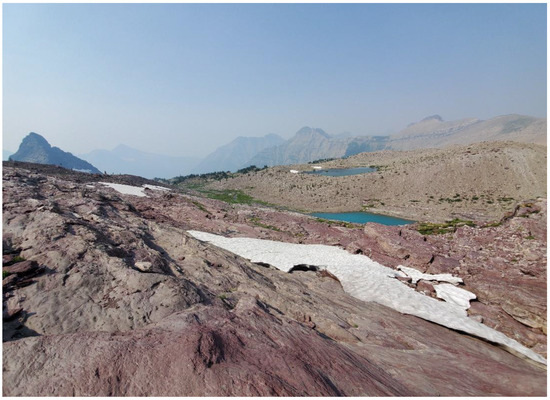
Figure 1.
Sperry Glacier’s foreland facing north toward the sparsely vegetated Little Ice Age terminal moraines.
The foreland environment supports patchy plant communities [49]. Approximately 1000 native plant species, including several rare, sensitive, and endemic species, are found in Glacier National Park across a diversity of ecological communities [49,50]. Of the 30 endemic species found in GNP, approximately half are found in alpine habitats [49]. The study area comprises plants characteristic of both subalpine and alpine plant communities and supports several endemic species, such as Penstemon ellipticus J.M. Coult. & Fisher and Hedysarum sulphurescens Rydb., which are commonly found in the subalpine meadows [49]. Additionally, wind-swept trees (e.g., Abies lasiocarpa (Hook.) Nutt.) and shrubs (e.g., Dryas spp.) characteristic of treeline and the wind-swept alpine zone are also found at Sperry Glacier’s foreland (personal observation and Carrara, 1989) [46]. Glaciers’ surface life is also an important component of glacial biodiversity and its response to glacier retreat [51,52]; however, these communities are not assessed here.
Wind is a primary dispersal mechanism of plants on glacier foreland [4,25]. Seeds can be trapped by surface roughness elements, including within concavities, rock fissures, and in the lee of boulders [24,53]. During our study, we observed plants growing in the shelter of these surface roughness elements (Figure 2). The moraines cap the furthest extent of the foreland and host a variety of tundra vegetation along with dwarf subalpine fir. The younger moraines, present at the edge of our study area, lack soil and host sparse pioneer species with an occasional subalpine fir, though vegetation is lacking compared to the older moraines [44]. The vegetation on this younger glacier foreland may be too sparse and heterogeneous to describe a clear vegetative community [49,54]. However, species such as P. ellipticus, Phacelia hastata Douglas ex Lehm., and Senecio fremontii Torr. & A. Gray are common across the talus-covered areas of the alpine zone [54]. Gentiana glauca Pall., a rare alpine perennial, grows near Sperry Glacier and is found nowhere else in GNP [49,50].
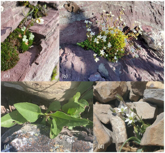
Figure 2.
Examples of vegetation establishment in a variety of microsites, including ledges (a), fissures (b), and rocks and boulders (c,d). Photos: A. Bryant 2022 and 2023.
2.2. Fieldwork Preparation and Methodology
Prior to conducting fieldwork, we used ArcGIS Pro (v. 2.8, ©ESRI, Redlands, CA, USA) to randomly generate sampling plot coordinates within the study area, ensuring a 50 m spacing between points. Due to accessibility and safety considerations, we confined our sampling to the southern portion of the glacier foreland (Figure 3). Glacier margin data were obtained from Fagre et al. (2017) [39] for 1966–2015 and Key et al. (2002) [38] for 1850–1966. The coordinates were uploaded to a Trimble Geo 7X GPS device with submeter accuracy for field navigation. In the field, we navigated to coordinates, ensuring representative sampling across five age range categories: 1850–1901, 1901–1927, 1927–1959, 1959–1993, and 1993–2023, with each category having similar temporal spans and plot numbers, though not identical due to margin dates not existing for every year (Figure 3). Four of the age ranges contain 25–35 years. No margin dates were available between 1850 and 1901, resulting in one group containing 51 years since it could not be further split.
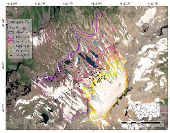
Figure 3.
Map of the study area, including Sperry Glacier and Sperry Glacier’s foreland with glacier margin dates and 61 sample plot locations spanning from the 1850 LIA moraine to the present glacier margin.
Field data collection occurred in July–August of 2021 and 2022 to coincide with minimal snow coverage (to allow the closest possible access to the glacier terminus) and the fruiting or flowering of many high-elevation plants in the region (to aid in species identification) [49]. GPS coordinates served as the centroids of 8 m2 sampling plots, which were used to delineate floristics and site data collection boundaries. In instances where coordinates were located within snowfields or unsafe and inaccessible areas, plots were repositioned by following a random compass heading for a random number of paces (between 1 and 25) and the blind toss of a surveyor stake. The coordinates and elevation of each new plot centroid were remeasured with the GPS.
Floristic data measured within each plot included species richness (number of different species per plot), percent vegetation and lichen cover, and community composition (Table 1). Percent cover was determined by estimating the proportion of the plot covered by the canopy, foliage, and bases of plants [55,56]. The proportion of area covered was based on the outermost outline of the vegetation from a vertical projection and considered overlap. To reduce subjectivity, the percent cover estimates were performed by two field team members simultaneously and averaged. All plant cover < 1% was categorized as 0.5%. To determine community composition, we identified plants to species level using Lesica (2002) [49] and Sullivan (2022) [57]. All species names were verified using the Integrated Taxonomic Information System (ITIS) to ensure the current taxonomic names were used. Since the identification of some taxa to species level requires magnification and no destructive sampling was permitted within the National Park boundaries, grasses, sedges, rushes, and mosses were identified to the family level. Lichens and all vegetation not identified down to species were grouped superficially into morphological kinds (i.e., grouped by physical appearance) to estimate species richness. Species richness in each plot was estimated by counting the number of species and the number of unique morphological kinds if not identified down to species.
Abiotic site variables measured at each plot allowed for characterization of fine-scale plant colonization sites. Percent surface rock fragment cover, which has relevance to plant survival, seed capture, and soil formation [25,26], was estimated in each plot for three clast size categories (fines–sands, gravel–cobble, and boulders) based on a modified Wentworth scale [58]. Observed concavity was a categorical variable that characterized each plot’s general topographic profile as straight, concave, convex, or undulating (Figure 4). Drainage classes for each plot were qualitatively estimated as poor, moderate, and well-drained. Depositional or erosional geomorphic process domains and landform types were additionally noted for each plot (Table 1).
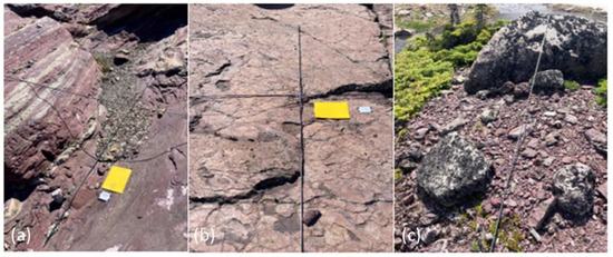
Figure 4.
A poorly drained, concave plot (a); poorly drained, straight plot (b); and moderately drained, convex plot (c). Photos: A. Bryant 2022.
2.3. Derived GIS Variables and Vegetation Indices
Abiotic conditions, such as slope, moisture, and solar radiation, can be inferred from topography using digital elevation models (DEMs). We thus derived a series of topographic variables to further characterize the landscape context that could influence vegetative growth and successional patterns [13,21,27,59,60,61]. These variables included Topographic Position Index (TPI), flow accumulation, profile and tangential curvature, solar radiation, slope angle, and aspect and were derived using ArcGIS Pro and open-source System for Automated Geoscientific Analyses (SAGA, Version 8.0) [62] from a USGS 1/3-arc sec National Elevation Dataset (NED) Digital Elevation Model (DEM) (~8.69 m × 8.69 m at the study area) obtained from USGS’s data download application available at https://apps.nationalmap.gov/downloader/ (accessed on 1 January 2024). Data for each variable were extracted by plot centroid using the projected coordinate system NAD_1983_UTM_Zone_12N.
Topographic position, measured by TPI, describes an area’s relative position within the surrounding landscape. TPI can influence erosion potential and soil development [63,64]. Sheltered locations are more likely to accumulate seeds and sediments, aiding vegetation establishment. Flow accumulation represents the accumulated weight of all cells from the DEM flowing into each downslope cell and is an indicator of water supply and erosion. Flow accumulation was calculated in ArcGIS using the deterministic infinity (D-infinity) method, which determines the flow direction at any angle toward the steepest slope. Surface curvature indicates the reflection (convex, positive curvature) or retention (concave, negative curvature) of water. We calculated two types of curvature: profile and tangential curvature. Profile curvature is the curvature parallel to the direction of the maximum slope, while tangential curvature is the curvature perpendicular to the direction of the maximum slope. Profile curvature influences how flow accelerates or decelerates down the slope [65], while tangential curvature influences how flow converges or diverges across an area [66]. Here, we consider both variables since they provide distinct information, although both variables are measures of how water and other resources move across the landscape. Area solar radiation (WH/m2) refers to annual insolation, or exposure to the sun’s radiation, across the landscape based on its topographic structure. Solar radiation, while essential for photosynthesis, can also cause desiccation, aided by the drying effects of wind, and variability in plant composition across alpine environments [13,67]. Slope, referring to slope steepness, impacts stability and disturbance events that can change plant succession dynamics [27]. Slope aspect influences the amount of solar radiation received at a site and affects vegetation cover and composition at glacier forelands [21]. The circular nature of the slope aspect (measured in degrees) necessitated a sine and cosine transformation to create measures of eastness and northness:
2.4. Vegetation Indices Calculation
We used field measurements of species richness and percent cover to calculate species evenness and the Shannon’s diversity index [68]. Species evenness is a measure of the relative abundance (or cover) of each species within a community. In this study, we used evenness to describe how evenly the percent cover estimates are distributed among each species [69]. Shannon’s diversity assesses the differences in biological variability over space or time, considering both species richness and evenness combined [70].

Table 1.
Independent variables used in this study with their collection method, units, and description/justification.
Table 1.
Independent variables used in this study with their collection method, units, and description/justification.
| Independent Variables | Source | Description/Justification |
|---|---|---|
| Terrain Age Ranges | Existing Geospatial Dataset | Dates of terrain exposure based on glacier margin date lines for analysis of vegetation over time [38,39]. |
| Drainage | Field | Drainage was categorized into poor and moderate drainage. Water availability is important for plant germination and survival [67]. |
| Observed Concavity | Field | Concavity was classified into concave, convex, straight, and undulating. Concavity can create safe sites [25]. |
| Landform feature | Field | Landform features were classified into moraines, Roche moutonnée, and others. These features may influence safe site availability. |
| % Fines–Sand | Field | The percent cover of surface fragments under 2 mm in size. These small surface fragments may contain nutrients and preserve moisture [26]. |
| % Gravel–Cobble | Field | The percent cover of surface fragments from 2 to 256 mm in size. Gravel and cobble provide safe sites [25,26]. |
| % Boulder | Field | The percent cover of surface fragments greater than 256 mm in size. Boulders provide shade and shelter from wind [26]. |
| Process Domain | Field | The main glacial process that shaped the landscape, classified as depositional or erosional [71]. |
| Northness | GIS-Derived | A cosine transformation of aspect, which may influence vegetation cover and composition [20]. |
| Eastness | GIS-Derived | A sine transformation of aspect, which may influence vegetation cover and composition [20]. |
| Slope (°) | GIS-Derived | A measure of the steepness of the surface. Steep slopes cause instability and may hinder vegetation development [6,26]. |
| Topographic Position Index | GIS-Derived | The relative position/elevation of a location. This position influences erosion and soil development [63,64]. |
| Flow Accumulation | GIS-Derived | The accumulated weight of water flow into each raster cell of a landscape. Flow accumulation influences the water supply in each plot. |
| Area Solar Radiation (WH/m2) | GIS-Derived | A measure of insolation, or solar exposure. Solar radiation may increase dehiscence or change plant composition [12,67]. |
| Profile Curvature (1/100 m) | GIS-Derived | The curvature parallel to the direction of the maximum slope. Profile curvature influences the acceleration and deceleration of flow [65]. |
| Tangential Curvature (1/100 m) | GIS-Derived | The curvature perpendicular to the direction of the maximum slope. Tangential curvature influences the convergence and divergence of flow [66]. |
2.5. Statistical Analyses
We used non-parametric Kruskal–Wallis tests with Dunn’s post hoc comparisons to assess differences in vegetation patterns (species richness, vegetation cover, Shannon’s diversity, and species evenness) across terrain age groups. Dunn’s test p-values were adjusted using the Holm method. General linear models (GLMs) were developed using backward stepwise selection in R Studio (v. 4.2.1) to identify the best explanatory variables for each response variable. Of the 16 initial explanatory variables (Table 1), slope steepness and northness were excluded due to collinearity with solar irradiance. Separate models were created for species richness, vegetation cover, Shannon’s diversity, and species evenness. The GLM family was chosen based on the response variable: Poisson for counts (species richness), binomial for proportions (vegetation cover, species evenness), and Gaussian for normally distributed data (Shannon’s diversity) (Tables S1 and S2. Models were selected based on the Akaike Information Criterion (AIC), Bayesian Information Criterion (BIC), and residual deviance, with the most parsimonious model chosen when values were similar. If no significant model emerged, the response variable was considered unexplained by the explanatory variables used in this study. The non-parametric Kruskal–Wallis multiple comparison test, followed by Dunn’s or Mann–Whitney U test as appropriate, was applied to assess relationships between explanatory and response variables, which were visualized with boxplots.
3. Results
3.1. Floristics and Chronosequence Patterns
Within the 61 plots, we found at least 93 morphologically distinct species, containing at least 46 distinct genera and 25 families in total. Among these, we identified 62 to the species level, including 41 identified genera and 23 identified families (Table 2 and Table S3).
Table 2.
Floristic synopsis of the families, genera, and species found in this study, including the number of plots and average vegetation cover (VC) found for the most prevalent species. The VC is averaged over all the plots in the study area and includes the standard deviation. This measurement of VC shows the likely cover of the vegetation across the entire foreland.
The dominant plant families, based on presence in plots, include Poaceae, Asteraceae, Polygonaceae, Cyperaceae, Plantaginaceae, and Saxifragaceae. Poaceae is the most prevalent family, appearing in 39 plots with an average VC of 2.19% ± 4.76%, followed by Asteraceae and Polygonaceae. Among the most prevalent species, Oxyria digyna (L.) Hill and S. fremontii are noteworthy, appearing in 21 and 18 plots, respectively, though their average coverage remains relatively low. Additionally, the presence of mosses and lichens is substantial. In particular, mosses are found in 34 plots with an average VC of 0.87% ± 1.79%, while lichens show a higher variability in coverage with an average VC of 1.30% ± 5.03%.
Each of these prevalent families and species, except for Plantaginaceae, P. ellipticus, and Arnica latifolia, occurred across the entire terrain age range. Moss was also prevalent across the entire terrain age range. Both P. ellipticus and A. latifolia were most commonly found in terrain exposed between 1850 and 1927, though they occasionally occurred on younger terrain (Table S3). Lichens were also absent from the most recently exposed terrain, only appearing on terrain exposed before 1993. The percent cover of lichen increased with terrain age, increasing from 0.07% in the 1927–1993 terrain age range to 1.17% in 1901–1927 and 5.23% in 1850–1901 (Table S3). Tree species, A. lasiocarpa and Picea engelmannii Parry ex Engelm., occurred in four plots, all located on older terrain and growing on moraines. The majority of species observed grew sparsely across the foreland. Thirty-five plant species occurred in a single plot, nine occurred in two plots, and ten occurred in three plots (Table S3).
Species richness and vegetation cover varied across the foreland (Table 3, Figure 5). We found species richness to be greater on older terrain (Figure 5) and to differ significantly among the terrain age categorical ranges (H(4) = 22.19, p < 0.001). A post hoc analysis of species richness using Dunn’s multiple comparison test and box plots revealed that species richness is significantly lower in the two most recent date ranges (1959–1993 and 1993–2022) than in the 1850–1901 (p = 0.005 and 0.003, respectively) and 1927–1959 date ranges (p = 0.030 and 0.026, respectively), with the mean richness increasing nearly 8-fold from the youngest to the oldest terrain age ranges (Table 3, Figure 5).
Table 3.
Number of plots in each age range; overall statistics for species richness (SR), Shannon’s diversity (SD), and species evenness (SE); averaged statistics per plot for SR, SD, SE, and vegetation cover (VC) (%) with standard deviations; and both species and absolute turnover represented by each range.
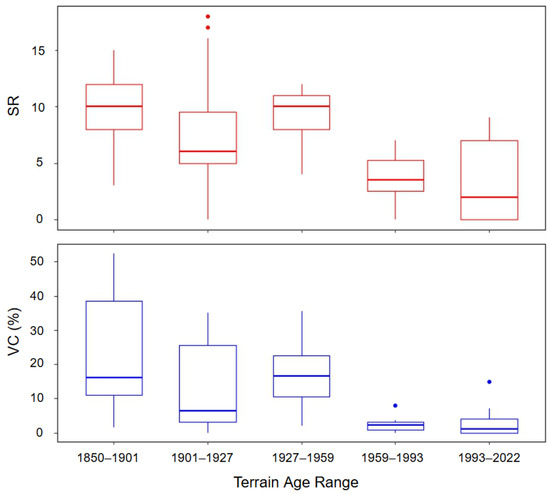
Figure 5.
Box plots depicting the distribution of vegetation cover (VC) (%) and species richness (SR) within terrain age ranges.
A total of 48 species were observed in the 1850–1901 terrain age range, 59 in 1901–1927, 36 in 1927–1959, 18 in 1959–1993, and 19 in 1993–2022 (Table 3). The mean percent vegetation per plot was 10.9%. The Kruskal–Wallis test revealed that vegetation cover differed significantly across the terrain age ranges (H(4) = 24.78, p < 0.0001). Post hoc comparisons indicated that vegetation cover in the two most recent age categories (1959–1993 and 1993–2022) was significantly lower compared to earlier periods. Specifically, vegetation cover in these recent categories was lower than in 1850–1901 (p = 0.003 and 0.001, respectively), 1901–1927 (p = 0.054 and 0.027), and 1927–1959 (p = 0.030 and 0.017), with the mean vegetation cover doubling from the youngest to oldest terrain age ranges (Table 3, Figure 5). A Kruskal–Wallis test revealed significant differences in both Shannon’s diversity (H(4) = 11.18, p = 0.025) and species evenness (H(4) = 20.15, p < 0.001) across terrain ages, though pairwise comparisons did not show significant differences between specific age groups. There may be a weak overall increase in Shannon’s diversity and decrease in species evenness across terrain age; however, this pattern is too weak to be verified with Dunn’s test. The average Shannon’s diversity per plot was 1.36 ± 0.72 SD, while the species evenness averaged 0.86 ± 0.14 SD (Table 3).
3.2. Generalized Linear Models
GLMs were informative for species richness and Shannon’s diversity, showing that these vegetative patterns can be partially explained by site variables collected in this study. Null models were best for explaining vegetation cover and species evenness, meaning none of the site characteristics improved the GLM’s ability to explain the variation in these indices, leaving the most parsimonious model to only include randomness as an explanation.
Species richness was best explained by drainage, terrain age, concavity, and the process domain. The model including these variables provides a much better fit to the data as evidenced by significantly lower AIC (316.49) and BIC (338) values compared to the null model’s AIC (429.86) and BIC (432) (Table 4 and Table S2). AIC and BIC are measures of model performance, where lower values indicate a better fit. Additionally, the residual deviance for the selected model is much lower (100.95) compared to the null model (232.32) (Table 4), suggesting that the chosen variables explain a large portion of the variation in species richness. The Kruskal–Wallis test further confirmed that species richness varied across drainage (H(1) = 22.38, p < 0.00001), terrain age (H(4) = 22.19, p < 0.001), concavity (H(3) = 8.12, p = 0.044), and the process domain (H(1) = 16.82, p < 0.001). Dunn’s test revealed higher species richness in concave plots compared to convex ones (p = 0.026), with the mean species richness in the concave plots (avg. 8.5 plants per plot) over double that in the convex plots (avg. 4 plants per plot) (Figure 6). Mann–Whitney U tests indicated that species richness was over twice as high in moderately drained plots (avg. 9.5 plants per plot) compared to poorly drained plots (avg. 4.1 plants per plot) (p < 0.001). Depositional landforms (avg. 9.8 plants per plot) also contained over double the species richness than that found in erosional landforms (avg. 4.6 plants per plot) (p < 0.001) (Figure 6).
Table 4.
The GLM null model and best model for species richness including values used to compare the models (i.e., AIC, BIC, degrees of freedom (D.F.), and residual deviance (Res. Dev.)). The estimate, standard error, and significance value of each variable were included for the best model.
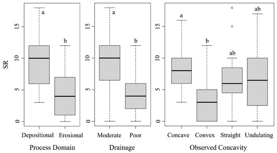
Figure 6.
Box plots showing the differences in species richness (SR) for each variable included in the best GLM model (for terrain age, see Figure 5). The letters depict post hoc test groups. Shared letters indicate ranges that are not significantly different, while different letters indicate a significant difference (p < 0.05).
Shannon’s diversity was best explained by drainage and concavity. The best GLM had lower AIC (41.103), BIC (52.7), and residual deviance (5.28) values compared to the null model’s AIC (58.055), BIC (61.9), and residual deviance (8.62) (Table 4 and Table S2). The Kruskal–Wallis test confirmed significant differences in Shannon’s diversity across drainage (H(1) = 12.03, p < 0.001) and concavity categories (H(3) = 14.70, p = 0.002). Dunn’s test showed greater diversity in concave than in convex plots (p < 0.001), with Shannon’s diversity in concave plots (avg. 1.8) double that of convex plots (0.9), and mild evidence that straight plots (avg. 1.4) have higher diversity than convex plots (p = 0.053), similar to the relationships seen between this variable and species richness in Figure 6. Mann–Whitney U tests indicated higher diversity in moderately drained plots (avg. 1.7) compared to poorly drained plots (avg. 1.1) (p < 0.001) (Figure 7).
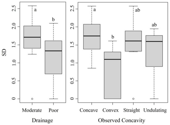
Figure 7.
Box plots showing the differences in Shannon’s diversity (SD) for each variable included in the best GLM model. The letters depict post hoc test groups. Shared letters indicate ranges that are not significantly different, while different letters indicate a significant difference (p < 0.05).
4. Discussion
4.1. Community Composition
We identified at least 93 morphologically distinct species, with 62 classified to the species level, representing 41 classified genera and 23 classified families (Table 2 and Table S3). These species were found across 61 sampling plots in Sperry Glacier’s foreland, with species per plot ranging from 0 to 18. Since grasses, rushes, sedges, and mosses were not identified to species level, this species count is likely conservative. All species recorded are native to Glacier National Park including three that are endemic to the Northern Rocky Mountains (Suksdorfia violacea A. Gray, Phacelia lyallii (A. Gray) Rydb., and P. ellipticus). Silene uralensis (Rupr.) Bocquet, Saxifraga rivularis L., and Woodsia oregana D.C. Eaton, also found in this study, have their status under review by the Montana Natural Heritage Program, meaning more data are required to make an accurate assessment of their risk level in Montana. Although Sperry Glacier is relatively remote, it is notable that no invasive, non-native plants were found in this study, especially considering the heavy visitation to other alpine areas in Glacier National Park, such as Grinnell Glacier.
Plants primarily with alpine distributions and those with a wide altitudinal distribution were found at Sperry Glacier, consistent with findings for the Grinnell Glacier foreland by Johnson (1980) [37]. Several of the most frequently encountered species, such as O. digyna, S. fremontii, and Epilobium anagallidifolium Lam., are distributed across subalpine to alpine environments, though several species are also found at lower montane elevations, such as P. ellipticus, Saxifraga bronchialis L. and Arnica latifolia Bong [49]. Oxyria digyna is found in mountain ranges around the world and is of ethnobotanical importance due to its pharmaceutical potential, nutritional value, and historical use [72]. Two nitrogen-fixing shrubs, Dryas drummondii Richardson ex Hook. and Dryas octopetala L. [73], grew on the moraines. Dryas octopetala, more commonly found at higher elevation than D. drummondii [49], was more prevalent at Sperry than D. drummondii.
The plant community across the foreland is spatially diverse, with many species only occurring in a few study plots. The diversity and infrequent occurrence of these species prevents the identification of a specific community composition of each terrain age range. However, some species, such as P. ellipticus, A. latifolia, and A. lasiocarpa, appear to favor older terrain. Lichen also appears to prefer older terrain. Lichen may be absent from younger terrain due to its proximity to nitrogen-rich meltwater [74,75], which limits lichen growth [76].
4.2. Diversity and Cover Change Across the Chronosequence
A major objective of this study was to characterize change in diversity metrics and cover across a chronosequence extending from the Little Ice Age (~1850) terminal moraine to the present glacier terminus. We found that terrain age impacted the vegetative metrics differently. Results of the Kruskal–Wallis and post hoc comparison tests revealed significant differences in both vegetation cover and species richness between the two most recent age categories and earlier time periods. Although the overall models were significant, post hoc pairwise comparisons did not reveal any significant differences in Shannon’s diversity or species evenness across the terrain age categories. These findings could suggest that while diversity and evenness vary across the entire terrain age spectrum, the differences across terrain age categories are not pronounced. The evenness values (Table 3) indicate a relatively balanced distribution of species among the sampling plots. averaging a species evenness of 0.86, which is comparable to that reported by Raffl et al. (2006) [31] for Rotmoosferner Glacier and Andreis et al. (2001) [19] for the Italian Alps.
Vegetation cover increased from 0% within 8 years of deglaciation to an average of 22.6% between 120 and 170 years (Table 3)—comparatively lower than cover observed at other glacier forelands [4,19,20,31]. For example, vegetation cover at Skaftafellsjökull in Southern Iceland reached 100% cover within 54 years [20], and Jamtalferner reached 80% cover after about 100 years [4]. The low vegetation cover is indicative of an isolated spatial pattern that may lead to more apomictic reproduction strategies that tend to lower genetic diversity [77] and lead to higher specialization of plants to certain conditions. A low genetic diversity may make adapting to new conditions more difficult and reduce some species’ ability to adjust to a changing climate [77]. Some species may be more strongly affected as the glacier melts and conditions change than others, depending on continued gene flow from incoming seeds or cross-pollination. Further investigation into the alpine population genetics and pollination mechanisms can help clarify which species are most at risk.
The average species richness (SR) within each terrain age ranges at its highest from 3.31 ± 0.28 species per plot (18 total species) within the 1993–2022 time period to 9.91 ± 0.32 species per plot (49 total species) within the 1850 to 1901 time period (Table 3). These results suggest that older terrains, which have likely undergone longer periods of ecological succession and stabilization, support higher biodiversity. This pattern is comparable to results reported for the Jamtalferner Glacier in the Austrian Alps, where species richness grew from 13 to 40–50 species over 100 years [4]. However, unlike Jamtalferner, where 13 species were observed within 2 years of deglaciation and doubled by year seven, Sperry foreland remained barren at these early stages. This comparatively delayed colonization rate has important implications regarding the ability of species to keep up with the rates of climate change [78]. Furthermore, the data from Sperry Glacier do not reflect a steady increase in plant species richness with increased terrain age; the highest total number of species (59 species) was recorded in plots deglaciated between 1901 and 1927, rather than in the oldest age range. Therefore, time since deglaciation is important, but it is not the only factor contributing to the observed vegetative patterns.
Vegetation cover and species richness patterns are interrelated along a successional gradient, shaped by changes in plant interactions over time. As vegetation cover increases, competition for space and resources intensifies, often leading to a decline in species richness as dominant species outcompete others [20,79]. This shift marks the transition from allogenic factors, such as environmental conditions, to autogenic factors, where species interactions primarily drive succession, as noted by Matthews (1992) [1].
Thus, delayed plant establishment, such as that seen on Sperry, can impact overall ecosystem development. At Sperry Glacier, species richness increased in light of consistently low vegetation cover (and presumably low interspecies competition) across the foreland, which peaked at 22.59% ± 1.57% cover after 170 years (Table 3). Other glacier forelands with higher vegetation cover often experience a peak and subsequent decline in species richness. Skaftafellsjökull Glacier in Southern Iceland, for example, reached 100% cover within 54 years, followed by a decline and plateau in species richness (presumably due to intensified competition) [20]. However, tropical glaciers like Humboldt in Venezuela exhibit much faster rates of colonization and support significantly higher vegetation cover and species richness [80]. This rapid ecosystem development and high vegetative measures are driven by a combination of warmer temperatures, higher productivity, and favorable niche dynamics [80,81]. Sperry’s slower increase in cover likely reduces competition pressures, allowing species richness to continue increasing over time (Figure 8). A reduced competition additionally suggests that Sperry remains in the allogenic phase of succession longer, where external factors (as opposed to species interactions) control plant establishment—a trend common in severe abiotic environments [1].
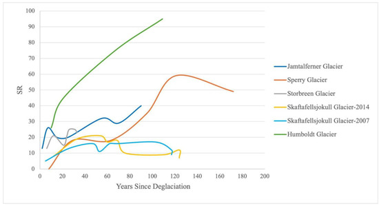
Figure 8.
A simplified interpretation of species richness (SR) trends over years since deglaciation from reported data in published glacial studies, including Sperry Glacier (this study), Jamtalferer Glacier in the Australian Eastern Alps [4], Skaftafellsjӧkull Glacier in Southern Iceland sampled in 2007 and 2014 [20], and Humboldt Glacier in Venezuela [80].
4.3. Biophysical Site Factors
We additionally assessed biophysical site factors (e.g., concavity, drainage, rock fragments, slope, aspect, terrain roughness) as possible contributors to plant diversity (Shannon’s diversity, species richness, and species evenness) and vegetation cover using GLMs. Terrain age has some influence on some of the biophysical site factors of the foreland. Moraines only occurred on older terrain, exposed between 1850 and 1959. The oldest terrain consisted mainly of depositional plots with moderate drainage while the younger terrain had mainly erosional plots with poor drainage. Each terrain age range, however, contained both depositional and erosional plots as well as poorly and moderately draining plots. Younger terrain also had slightly less solar irradiance and greater flow accumulation than the older terrain ranges. These biophysical site factors, though influenced by terrain age, vary across the foreland within each terrain age, making them important variables to study apart from terrain age.
Only models predicting variation in species richness and Shannon’s diversity were meaningful. In addition to terrain age, the GLMs revealed that some field-derived variables—process domain, drainage, and observed concavity—explained variation in species richness and Shannon diversity, whereas GIS-derived terrain surface measures, including TPI and the two measures of curvature, did not. However, the effects between the two diversity measures differ in magnitude and significance. For both SR and SD, poor drainage and convex terrain have a statistically significant negative effect on the number of species and Shannon’s diversity. These effects are more pronounced for SR, which has additional significant negative effects from straight (flat) and undulating terrain categories (Table 4; Figure 6). Additionally, terrain age is an important predictor for SR but is not for SD, indicating that species richness, but not Shannon Diversity (which considers number of species, species’ percent cover, and species evenness), varies considerably across terrain age, supporting the idea that terrain age is not the main factor affecting diversity or evenness (Table 2). Overall, the models suggest that both richness and diversity, as measured by Shannon diversity, are shaped by the process domain, drainage, and concavity, but species richness is more sensitive to a broader range of predictors. The main factors revealed by the models to explain species richness and Shannon’s diversity variation were all field-derived while none of the GIS-derived variables were significant in the models. Not only do field-derived variables have a greater resolution, but they also more precisely reflect aspects of the plot’s microtopography, demonstrating the continued importance of field data collection and verification along with the need for higher-resolution DEMs at glacial studies for modeling fine-scale vegetation processes.
Study plots were dominated by erosional and depositional geomorphic domains (Figure 1), meaning that most plots were characterized by landforms created by glacial erosional processes that resulted from landscape scouring and resultant features, or depositional processes that resulted from the deposition of ground till or moraines. No active periglacial processes were observed, which contrasts with Eichel et al. (2013) [82] for the Turtmann Glacier forefield in Switzerland. Landforms created by these two process domains can substantially impact the microsites available for plant colonization. Erosional plots tend to have fewer sheltering features (e.g., surface till), though the topography still varies (e.g., concavity). Depositional plots have substantial surface till due to glaciers depositing these fragments at the ends or sides of the glacier’s extent as it melts, forming terminal and lateral moraines. These depositional process domains are positively associated with higher species richness (Table 4; Figure 6). The overall shelter of these depositional plots may allow more species to establish due to an increased sheltering capacity and accumulate resources [25], increasing the species richness relative to erosional plots.
Drainage categorization gives insight into how water interacts with the microtopography. Our plots contained poor and moderately draining plots. Due to the lack of soil horizon, there were no well-draining plots in the foreland. Water either pooled in or ran directly off of poorly draining plots, while moderately draining plots slowed down and retained some water without causing severe pooling (Figure 4). At Sperry Glacier’s foreland, poor drainage was negatively associated with both species richness (Table 4; Figure 6) and Shannon’s diversity (Table 5; Figure 7). Pooling may drown established vegetation, and fast runoff may wash seeds away before they can establish. This would limit the number and diversity of plants that can grow in poorly draining plots, resulting in greater species richness and Shannon’s diversity in the moderately draining plots. This finding aligns with Matthews and Vater (2015) [9], who found that water initially dominated the allogenic phase in succession and with the idea that erosional areas, where soil and nutrients are regularly displaced, provide more unstable environments, limiting the establishment and persistence of species.
Table 5.
GLM null model and best model for Shannon’s diversity (SD), including values used to compare the models (i.e., AIC, BIC, degrees of freedom (D.F.), and residual deviance (Res. Dev.)). The estimate, standard error, and significance value of each variable were included for the best model.
The observed concavity classified the nature of the immediate surface topography within the plot. Concave plots were positively associated, while convex plots were negatively associated with both species richness (Table 4; Figure 6) and Shannon’s diversity (Table 5; Figure 7), suggesting that concave landforms promote species richness and diversity, possibly due to water and sediment catching potential and slight sheltering. Convex terrain characteristics could create harsher or less stable microclimates, reducing their capacity to support a wide variety of species. Using these models, plots with depositional characteristics, moderate drainage, and an overall concave shape appear to foster a greater species richness (Table 4; Figure 6) and Shannon’s diversity (Table 5; Figure 7).
Plant colonization patterns and vegetation community development at Sperry Glacier do not strictly follow patterns that may be expected solely on terrain age. Factors such as microtopography (through the provision of safe sites and concave sites where substrate and moisture can accumulate) appear influential in driving the measured vegetation patterns. Atmospheric changes associated with climate drivers influence carbon (CO2), nitrogen, and sulfur (SO2) cycles at these sites via fine particle pollution carried by wind and deposited into these environments [83], likely accumulated by these safe sites. Additional sources of nutrients likely originate from bedrock erosion [84] and meltwater. Meltwater carries nitrogen and phosphorus from glaciers and snowfields, which accumulate these resources from the surrounding rock, rain, and windblown particles [74,75,84,85]. Access to these resources may rely on proximity to the glacier and snowfields [75] as well as the microtopography’s ability to capture the meltwater. The weathering of the bedrock may be especially important for the availability of phosphorus [84]. Plant growth response to these scarce resources on the landscape may influence growth as these nutrient limitations are reduced [83,86,87].
Furthermore, the geomorphic context of Sperry Glacier, dominated by large areas of exposed, consolidated bedrock with minimal soil formation, contributes significantly to the lag in community development, as compared to results reported in other studies (Figure 8). Most of the limited soil is confined to cracks or around established roots, restricting the potential for new plants to take hold. The lack of a well-developed soil horizon in these forelands—unlike the conditions described in other studies from mid-latitudes [16,67]—hinders successional processes and limits plant cover [19,78]. Colonizing plants affect the landscape by capturing sediment [88], changing the soil nutrients [89], and facilitating other plants [7], and thus the investigation of a threshold effect to vegetation colonization under different geographic contexts could be insightful, especially in light of climate change responses. The unique geographic context of Sperry Glacier may prevent timely adaptive response to rapidly changing environmental and climate conditions, potentially leading to the extinction of some species, changing the community, reducing ecosystem services [78], and creating novel ecosystems in the wake of glacier retreat [90], an outcome to which topographic contexts at glacier forefronts may contribute.
5. Conclusions
Overall, we found both terrain age and biophysical site factors are important for understanding vegetative patterns across Sperry Glacier’s foreland; however, different vegetative indices are influenced differently. Accessing these patterns across the terrain age ranges shows the importance terrain age plays on species richness and vegetation cover while the GLMs underscore the importance of environmental factors in explaining species richness and Shannon’s diversity trends. Meanwhile, none of the variables investigated in this study significantly explained species evenness. Among the significant variables, older terrains, better drainage, and less exposed terrain features (i.e., concave plots and depositional plots) are associated with higher diversity measures (i.e., species richness, Shannon’s diversity, or both), reflecting the influence of both long-term ecological development and stable environmental conditions on biodiversity. The negative impacts of poor drainage and erosional processes further highlight the role of landscape stability in supporting biodiversity. These findings offer valuable insights into the ecological dynamics of terrain age and physical geography, with implications for conservation strategies in rapidly changing environments.
Supplementary Materials
The following supporting information can be downloaded at: https://www.mdpi.com/article/10.3390/land14020306/s1. Table S1: Comparison of species richness (SR) models evaluated in the backward stepwise selection process, starting with a model containing all the variables and ending with the null model. The second column shows what variables were removed or added from the model in the previous row to create the current model. Each model was compared based on the Akaike Information Criterion (AIC), Bayesian Information Criterion (BIC), degrees of freedom (D.F.) and residual deviance (Res. Dev). Table S2: Comparison of Shannon’s Diversity (SD) models evaluated in the backward stepwise selection process, starting with a model containing all the variables and ending with the null model. The second column shows what variables were removed or added from the model in the previous row. Each model was compared based on the Akaike Information Criterion (AIC), Bayesian Information Criterion (BIC), degrees of freedom (D.F.) and residual deviance (Res. Dev). Table S3: List of all species observed, number of associated plots, and average % cover, by species, within each terrain age range.
Author Contributions
Conceptualization, L.M.R. and A.B.; methodology, A.B., L.M.R., D.G., and T.P.; formal analysis, A.B., L.M.R., and T.P.; writing—original draft preparation, A.B. and L.M.R.; writing—review and editing, A.B., L.M.R., D.G., and T.P.; visualization, A.B. and T.P.; supervision, L.M.R., D.G., and T.P. All authors have read and agreed to the published version of the manuscript.
Funding
This research received no external funding.
Data Availability Statement
The raw field data supporting the conclusions of this article may be made available by the authors upon reasonable request.
Acknowledgments
The Department of Geography at Virginia Tech provided internal financial support for the fieldwork through the Sidman P. Poole Endowment. We thank the National Park Service for their permitting and logistical support.
Conflicts of Interest
The authors declare no conflicts of interest. The funders had no role in the design of this study, in the collection, analysis, or interpretation of data, in the writing of the manuscript, or in the decision to publish the results.
References
- Matthews, J.A. The Ecology of Recently-Deglaciated Terrain: A Geoecological Approach to Glacier Forelands; Cambridge University Press: Cambridge, UK, 1992. [Google Scholar]
- Fickert, T. Glacier Forelands-Unique Field Laboratories for the Study of Primary Succession of Plants. In Glacier Evolution in a Changing World; Godone, D., Ed.; InTech: Rijeka, Croatia, 2017; pp. 125–146. [Google Scholar]
- Bosson, J.-B.; Huss, M.; Cauvy-Fraunié, S.; Clément, J.-C.; Costes, G.; Fischer, M.; Poulenard, J.; Arthaud, F. Future Emergence of New Ecosystems Caused by Glacial Retreat. Nature 2023, 620, 562–569. [Google Scholar] [CrossRef] [PubMed]
- Fischer, A.; Fickert, T.; Schwaizer, G.; Patzelt, G.; Groß, G. Vegetation Dynamics in Alpine Glacier Forelands Tackled from Space. Sci. Rep. 2019, 9, 13918. [Google Scholar] [CrossRef] [PubMed]
- Ficetola, G.F.; Marta, S.; Guerrieri, A.; Gobbi, M.; Ambrosini, R.; Fontaneto, D.; Zerboni, A.; Poulenard, J.; Caccianiga, M.; Thuiller, W. Dynamics of Ecological Communities Following Current Retreat of Glaciers. Annu. Rev. Ecol. Evol. Syst. 2021, 52, 405–426. [Google Scholar] [CrossRef]
- Lambert, C.B.; Resler, L.M.; Shao, Y.; Butler, D.R. Vegetation Change as Related to Terrain Factors at Two Glacier Forefronts, Glacier National Park, Montana, USA. J. Mt. Sci. 2020, 17, 1–15. [Google Scholar] [CrossRef]
- Erschbamer, B.; Schlag, R.N.; Winkler, E. Colonization Processes on a Central Alpine Glacier Foreland. J. Veg. Sci. 2008, 19, 855–862. [Google Scholar] [CrossRef]
- Cazzolla Gatti, R.; Dudko, A.; Lim, A.; Velichevskaya, A.I.; Lushchaeva, I.V.; Pivovarova, A.V.; Ventura, S.; Lumini, E.; Berruti, A.; Volkov, I.V. The Last 50 Years of Climate-induced Melting of the Maliy Aktru Glacier (Altai Mountains, Russia) Revealed in a Primary Ecological Succession. Ecol. Evol. 2018, 8, 7401–7420. [Google Scholar] [CrossRef]
- Matthews, J.A.; Vater, A.E. Pioneer Zone Geo-Ecological Change: Observations from a Chronosequence on the Storbreen Glacier Foreland, Jotunheimen, Southern Norway. CATENA 2015, 135, 219–230. [Google Scholar] [CrossRef]
- Losapio, G.; Cerabolini, B.E.L.; Maffioletti, C.; Tampucci, D.; Gobbi, M.; Caccianiga, M. The Consequences of Glacier Retreat Are Uneven Between Plant Species. Front. Ecol. Evol. 2021, 8, 616562. [Google Scholar] [CrossRef]
- Mori, A.S.; Osono, T.; Uchida, M.; Kanda, H. Changes in the Structure and Heterogeneity of Vegetation and Microsite Environments with the Chronosequence of Primary Succession on a Glacier Foreland in Ellesmere Island, High Arctic Canada. Ecol. Res. 2008, 23, 363–370. [Google Scholar] [CrossRef]
- Schumann, K.; Gewolf, S.; Tackenberg, O. Factors Affecting Primary Succession of Glacier Foreland Vegetation in the European Alps. Alp. Bot. 2016, 126, 105–117. [Google Scholar] [CrossRef]
- Eichel, J.; Draebing, D.; Winkler, S.; Meyer, N. Similar Vegetation-geomorphic Disturbance Feedbacks Shape Unstable Glacier Forelands across Mountain Regions. Ecosphere 2023, 14, e4404. [Google Scholar] [CrossRef]
- Young, K. Ecology of Land Cover Change in Glaciated Tropical Mountains. Rev. Peru. Biol. 2014, 21, 259–270. [Google Scholar] [CrossRef][Green Version]
- Cauvy-Fraunié, S.; Dangles, O. A Global Synthesis of Biodiversity Responses to Glacier Retreat. Nat. Ecol. Evol. 2019, 3, 1675–1685. [Google Scholar] [CrossRef] [PubMed]
- Wojcik, R.; Eichel, J.; Bradley, J.A.; Benning, L.G. How Allogenic Factors Affect Succession in Glacier Forefields. Earth-Sci. Rev. 2021, 218, 103642. [Google Scholar] [CrossRef]
- Chapin, F.S.; Walker, L.R.; Fastie, C.L.; Sharman, L.C. Mechanisms of Primary Succession Following Deglaciation at Glacier Bay, Alaska. Ecol. Monogr. 1994, 64, 149–175. [Google Scholar] [CrossRef]
- Walker, L.R.; Wardle, D.A.; Bardgett, R.D.; Clarkson, B.D. The Use of Chronosequences in Studies of Ecological Succession and Soil Development. J. Ecol. 2010, 98, 725–736. [Google Scholar] [CrossRef]
- Andreis, C.; Caccianiga, M.; Cerabolini, B. Vegetation and Environmental Factors during Primary Succession on Glacier Forelands: Some Outlines from the Italian Alps. Plant Biosyst. 2001, 135, 295–310. [Google Scholar] [CrossRef]
- Glausen, T.G.; Tanner, L.H. Successional Trends and Processes on a Glacial Foreland in Southern Iceland Studied by Repeated Species Counts. Ecol. Process. 2019, 8, 11. [Google Scholar] [CrossRef]
- Pickett, S.T.A. Space-for-Time Substitution as an Alternative to Long-Term Studies. In Long-Term Studies in Ecology: Approaches and Alternatives; Likens, G.E., Ed.; Springer: New York, NY, USA, 1989; pp. 110–135. [Google Scholar]
- Malanson, G.P.; Butler, D.R.; Fagre, D.B.; Walsh, S.J.; Tomback, D.F.; Daniels, L.D.; Resler, L.M.; Smith, W.K.; Weiss, D.J.; Peterson, D.L. Alpine Treeline of Western North America: Linking Organism-to-Landscape Dynamics. Phys. Geogr. 2007, 28, 378–396. [Google Scholar] [CrossRef]
- Carrara, P.E.; McGimsey, R.G. The Late-Neoglacial Histories of the Agassiz and Jackson Glaciers, Glacier National Park, Montana. Arct. Alp. Res. 1981, 13, 183–196. [Google Scholar] [CrossRef]
- Resler, L.M. Geomorphic Controls of Spatial Pattern and Process at Alpine Treeline. Prof. Geogr. 2006, 58, 124–138. [Google Scholar] [CrossRef]
- Jumpponen, A.; Väre, H.; Mattson, K.G.; Ohtonen, R.; Trappe, J.M. Characterization of ‘Safe Sites’ for Pioneers in Primary Succession on Recently Deglaciated Terrain. J. Ecol. 1999, 87, 98–105. [Google Scholar] [CrossRef]
- Perez, F. Phytogeomorphic Influence of Stone Covers and Boulders on Plant Distribution and Slope Processes in High-Mountain Areas. Geogr. Compass 2009, 3, 1774–1803. [Google Scholar] [CrossRef]
- Raven, P.; Evert, R.; Eichhorn, S. Biology of Plants, 7th ed.; WH Freedman and Company Worth Publishers: New York, NY, USA, 1999. [Google Scholar]
- Grohmann, C.; Hartmann, J.N.; Kovalev, A.; Gorb, S.N. Dandelion Diaspore Dispersal: Frictional Anisotropy of Cypselae of Taraxacum officinale Enhances Their Interlocking with the Soil. Plant Soil 2019, 440, 399–408. [Google Scholar] [CrossRef]
- Bayle, A. A Recent History of Deglaciation and Vegetation Establishment in a Contrasted Geomorphological Context, Glacier Blanc, French Alps. J. Maps 2020, 16, 766–775. [Google Scholar] [CrossRef]
- Fickert, T. Common Patterns and Diverging Trajectories in Primary Succession of Plants in Eastern Alpine Glacier Forelands. Diversity 2020, 12, 191. [Google Scholar] [CrossRef]
- Raffl, C.; Mallaun, M.; Mayer, R.; Erschbamer, B. Vegetation Succession Pattern and Diversity Changes in a Glacier Valley, Central Alps, Austria. Arct. Antarct. Alp. Res. 2006, 38, 421–428. [Google Scholar] [CrossRef]
- Moreau, M.; Laffly, D.; Joly, D.; Brossard, T. Analysis of Plant Colonization on an Arctic Moraine since the End of the Little Ice Age Using Remotely Sensed Data and a Bayesian Approach. Remote Sens. Environ. 2005, 99, 244–253. [Google Scholar] [CrossRef]
- Rydgren, K.; Halvorsen, R.; Töpper, J.P.; Njøs, J.M. Glacier Foreland Succession and the Fading Effect of Terrain Age. J. Veg. Sci. 2014, 25, 1367–1380. [Google Scholar] [CrossRef]
- Pauli, H.; Gottfried, M.; Reiter, K.; Klettner, C.; Grabherr, G. Signals of Range Expansions and Contractions of Vascular Plants in the High Alps: Observations (1994–2004) at the GLORIA* Master Site Schrankogel, Tyrol, Austria. Glob. Change Biol. 2007, 13, 147–156. [Google Scholar] [CrossRef]
- Brown, J.; Harper, J.; Humphrey, N. Cirque Glacier Sensitivity to 21st Century Warming: Sperry Glacier, Rocky Mountains, USA. Glob. Planet. Change 2010, 74, 91–98. [Google Scholar] [CrossRef]
- Goff, P.; Butler, D.R. James Dyson (1948) Shrinkage of Sperry and Grinnell Glaciers, Glacier National Park, Montana. Geographical Review 38(1): 95–103. Prog. Phys. Geogr. 2016, 40, 616–621. [Google Scholar] [CrossRef]
- Johnson, A. Grinnell and Sperry Glaciers, Glacier National Park, Montana: A Record of Vanishing Ice, Professional Paper, Report 1180; U.S. Geological Survey: Reston, VA, USA, 1980. [Google Scholar]
- Key, C.H.; Fagre, D.B.; Menicke, R.K. Glacier Retreat in Glacier National Park, Montana. US Geol. Surv. Prof. Pap. 2002, 1386, 365. [Google Scholar]
- Fagre, D.; McKeon, L.; Dick, L.; Fountain, A. Glacier Margin Time Series (1966, 1998, 2005, 2015) of the Named Glaciers of Glacier National Park, MT, USA; US Geological Survey Data Release: Reston, VA, USA, 2017. [Google Scholar]
- Walker, L.; Del Moral, R. Primary Succession and Ecosystem Rehabilitation; Cambridge University Press: Cambridge, UK, 2003. [Google Scholar]
- Matthes, F.E. Committee on Glaciers, 1939–40. Eos Trans. Am. Geophys. Union 1940, 21, 396–406. [Google Scholar]
- Hall, M.H.; Fagre, D.B. Modeled Climate-Induced Glacier Change in Glacier National Park, 1850–2100. BioScience 2003, 53, 131–140. [Google Scholar] [CrossRef]
- Selkowitz, D.J.; Fagre, D.B.; Reardon, B.A. Interannual Variations in Snowpack in the Crown of the Continent Ecosystem. Hydrol. Process. 2002, 16, 3651–3665. [Google Scholar] [CrossRef]
- Carrara, P.E. Late Quaternary Glacial and Vegetative History of the Glacier National Park Region, Montana; USGPO: Pueblo, CO, USA, 1989. [Google Scholar]
- Dyson, J.L. Shrinkage of Sperry and Grinnell Glaciers, Glacier National Park, Montana. Geogr. Rev. 1948, 38, 95–103. [Google Scholar] [CrossRef]
- Wang, T.; Hamann, A.; Spittlehouse, D.; Carroll, C. Locally Downscaled and Spatially Customizable Climate Data for Historical and Future Periods for North America. PloS ONE 2016, 11, e0156720. [Google Scholar] [CrossRef] [PubMed]
- Whipple, J.W. Geologic Map of Glacier National Park, Montana; U.S. Geological Survey: Reston, VA, USA, 1992.
- Carrara, P.E.; McGimsey, R.G. Map Showing Distribution of Moraines and Extent of Glaciers from the Mid-19th Century to 1979 in the Mount Jackson Area, Glacier National Park, Montana; U.S. Geological Survey: Reston, VA, USA, 1988.
- Lesica, P. Flora of Glacier National Park, Montana; Oregon State University Press: Corvallis, OR, USA, 2002. [Google Scholar]
- Mauer, B.; Williams, T. An Analysis of Potential Sensitive Plant Species for Long-Term Monitoring in Glacier National Park. UW-Natl. Park Serv. Res. Stn. Annu. Rep. 1991, 15, 105–114. [Google Scholar] [CrossRef]
- Stibal, M.; Bradley, J.A.; Edwards, A.; Hotaling, S.; Zawierucha, K.; Rosvold, J.; Lutz, S.; Cameron, K.A.; Mikucki, J.A.; Kohler, T.J. Glacial Ecosystems Are Essential to Understanding Biodiversity Responses to Glacier Retreat. Nat. Ecol. Evol. 2020, 4, 686–687. [Google Scholar] [CrossRef]
- Fickert, T.; Friend, D.; Molnia, B.; Grüninger, F.; Richter, M. Vegetation Ecology of Debris-Covered Glaciers (DCGs)—Site Conditions, Vegetation Patterns and Implications for DCGs Serving as Quaternary Cold-and Warm-Stage Plant Refugia. Diversity 2022, 14, 114. [Google Scholar] [CrossRef]
- Kondo, K.; Tsuchiya, M.; Sanada, S. Evaluation of Effect of Micro-Topography on Design Wind Velocity. J. Wind Eng. Ind. Aerodyn. 2002, 90, 1707–1718. [Google Scholar] [CrossRef]
- Damm, C. A Phytosociological Study of Glacier National Park, Montana, USA, with Notes on the Syntaxonomy of Alpine Vegetation in Western North America. Ph.D. Thesis, Georg-August Universitaet, Goettingen, Germany, 2001. [Google Scholar]
- Schulz, B. Sampling and Estimation Procedures for the Vegetation Diversity and Structure Indicator; US Department of Agriculture, Forest Service, Pacific Northwest Research Station, Portland, OR, USA, 2009.
- Godínez-Alvarez, H.; Herrick, J.E.; Mattocks, M.; Toledo, D.; Van Zee, J. Comparison of Three Vegetation Monitoring Methods: Their Relative Utility for Ecological Assessment and Monitoring. Ecol. Indic. 2009, 9, 1001–1008. [Google Scholar] [CrossRef]
- Sullivan, S.K. Glacier NP Wildflowers. 2022. Available online: https://play.google.com/store/apps/details?id=com.wildflowersearch.glwildflowers&hl=en_US&gl=US (accessed on 1 July 2022).
- Wentworth, C.K. A Scale of Grade and Class Terms for Clastic Sediments. J. Geol. 1922, 30, 377–392. [Google Scholar] [CrossRef]
- Brown, D.G. Comparison of Vegetation-Topography Relationships at the Alpine Treeline Ecotone. Phys. Geogr. 1994, 15, 125–145. [Google Scholar] [CrossRef]
- Guisan, A.; Theurillat, J.; Kienast, F. Predicting the Potential Distribution of Plant Species in an Alpine Environment. J. Veg. Sci. 1998, 9, 65–74. [Google Scholar] [CrossRef]
- Smith-Mckenna, E.K.; Resler, L.M.; Tomback, D.F.; Zhang, H.; Malanson, G.P. Topographic Influences on the Distribution of White Pine Blister Rust in Pinus albicaulis Treeline Communities. Écoscience 2013, 20, 215–229. [Google Scholar] [CrossRef]
- Conrad, O.; Bechtel, B.; Bock, M.; Dietrich, H.; Fischer, E.; Gerlitz, L.; Wehberg, J.; Wichmann, V.; Böhner, J. System for Automated Geoscientific Analyses (SAGA) v. 8.0. Geosci. Model Dev. 2015, 8, 1991–2007. [Google Scholar] [CrossRef]
- Román-Sánchez, A.; Vanwalleghem, T.; Peña, A.; Laguna, A.; Giráldez, J.V. Controls on Soil Carbon Storage from Topography and Vegetation in a Rocky, Semi-Arid Landscapes. Geoderma 2018, 311, 159–166. [Google Scholar] [CrossRef]
- Temme AJ, A.M.; Heckmann, T.; Harlaar, P. Silent Play in a Loud Theatre—Dominantly Time-Dependent Soil Development in the Geomorphically Active Proglacial Area of the Gepatsch Glacier, Austria. CATENA 2016, 147, 40–50. [Google Scholar] [CrossRef]
- Buckley, A. Understanding Curvature Raster. ArcGIS Blog. Available online: https://www.esri.com/arcgis-blog/products/product/imagery/understanding-curvature-rasters/ (accessed on 1 July 2022).
- Kopp, S.; New Surface Analysis Capabilities in ArcGIS Pro 2.7. ArcGIS Blog. Available online: https://www.esri.com/arcgis-blog/products/arcgis-pro/analytics/new-slope-aspect-curvature/ (accessed on 1 July 2022).
- Erschbamer, B.; Caccianiga, M.S. Glacier Forelands: Lessons of Plant Population and Community Development. Prog. Bot. 2017, 78, 259–284. [Google Scholar]
- Shannon, C.E. A Mathematical Theory of Communication. Bell Syst. Tech. J. 1948, 27, 379–423. [Google Scholar] [CrossRef]
- Moore, J.C. Diversity, Taxonomic versus Functional. In Encyclopedia of Biodiversity, 2nd ed.; Levin, S.A., Ed.; Academic Press: Waltham, MA, USA, 2013; pp. 648–656. [Google Scholar]
- Ortiz-Burgos, S. Shannon-Weaver Diversity Index. In Encyclopedia of Estuaries; Kennish, M.J., Ed.; Springer: Dordrecht, The Netherlands, 2016; pp. 572–573. [Google Scholar]
- Eichel, J. Vegetation Succession and Biogeomorphic Interactions in Glacier Forelands. In Geomorphology of Proglacial Systems: Landform and Sediment Dynamics in Recently Deglaciated Alpine Landscapes; Heckmann, T., Morche, D., Eds.; Springer International Publishing: Cham, Switzerland, 2019; pp. 327–349. [Google Scholar]
- Ahmad, I.; Milella, L.; Alotaibi, G. Oxyria digyna: A Review on the Nutritional Value, Phytochemistry and Ethnopharmacology. PHYTONutrients 2022, 1, 2–16. [Google Scholar] [CrossRef]
- Billault-Penneteau, B.; Sandré, A.; Folgmann, J.; Parniske, M.; Pawlowski, K. Dryas as a Model for Studying the Root Symbioses of the Rosaceae. Front. Plant Sci. 2019, 10, 661. [Google Scholar] [CrossRef] [PubMed]
- Bowman, W.D. Inputs and Storage of Nitrogen in Winter Snowpack in an Alpine Ecosystem. Arct. Alp. Res. 1992, 24, 211–215. [Google Scholar] [CrossRef]
- Björk, R.G.; Molau, U. Ecology of Alpine Snowbeds and the Impact of Global Change. Arct. Antarct. Alp. Res. 2007, 39, 34–43. [Google Scholar] [CrossRef]
- Soudzilovskaia, N.; Onipchenko, V.; Cornelissen, J.; Aerts, R. Biomass Production, N:P Ratio and Nutrient Limitation in a Caucasian Alpine Tundra Plant Community. J. Veg. Sci. 2005, 16, 399–406. [Google Scholar] [CrossRef]
- Jump, A.S.; Peñuelas, J. Running to Stand Still: Adaptation and the Response of Plants to Rapid Climate Change. Ecol. Lett. 2005, 8, 1010–1020. [Google Scholar] [CrossRef] [PubMed]
- Zimmer, A.; Meneses, R.I.; Rabatel, A.; Soruco, A.; Dangles, O.; Anthelme, F. Time Lag between Glacial Retreat and Upward Migration Alters Tropical Alpine Communities. Perspect. Plant Ecol. Evol. Syst. 2018, 30, 89–102. [Google Scholar] [CrossRef]
- Jones, G.A.; Henry, G.H.R. Primary Plant Succession on Recently Deglaciated Terrain in the Canadian High Arctic. J. Biogeogr. 2003, 30, 277–296. [Google Scholar] [CrossRef]
- Llambí, L.D.; Melfo, A.; Gámez, L.E.; Pelayo, R.C.; Cárdenas, M.; Rojas, C.; Torres, J.E.; Ramírez, N.; Huber, B.; Hernández, J. Vegetation Assembly, Adaptive Strategies and Positive Interactions During Primary Succession in the Forefield of the Last Venezuelan Glacier. Front. Ecol. Evol. 2021, 9, 657755. [Google Scholar] [CrossRef]
- Brown, J.H. Why Are There so Many Species in the Tropics? J. Biogeogr. 2014, 41, 8–22. [Google Scholar] [CrossRef] [PubMed]
- Eichel, J.; Krautblatter, M.; Schmidtlein, S.; Dikau, R. Biogeomorphic Interactions in the Turtmann Glacier Forefield, Switzerland. Geomorphology 2013, 201, 98–110. [Google Scholar] [CrossRef]
- Dawes, M.A.; Hagedorn, F.; Handa, I.T.; Streit, K.; Ekblad, A.; Rixen, C.; Körner, C.; Hättenschwiler, S. An Alpine Treeline in a Carbon Dioxide-Rich World: Synthesis of a Nine-Year Free-Air Carbon Dioxide Enrichment Study. Oecologia 2013, 171, 623–637. [Google Scholar] [CrossRef] [PubMed]
- Föllmi, K.B.; Hosein, R.; Arn, K.; Steinmann, P. Weathering and the Mobility of Phosphorus in the Catchments and Forefields of the Rhône and Oberaar Glaciers, Central Switzerland: Implications for the Global Phosphorus Cycle on Glacial–Interglacial Timescales. Geochim. Cosmochim. Acta 2009, 73, 2252–2282. [Google Scholar] [CrossRef]
- Agustina, R.; Nicolás, M.R.; Luis, E.B.; Guido, B.; Eleonora, C. Rock Glacier and Solifluction Lobes Groundwater as Nutrient Sources and Refugia for Unique Macroinvertebrate Assemblages in a Mountain Ecosystem of the North Patagonian Andes. Aquat. Sci. 2024, 86, 11. [Google Scholar] [CrossRef]
- Körner, C. The Nutritional Status of Plants from High Altitudes: A Worldwide Comparison. Oecologia 1989, 81, 379–391. [Google Scholar] [CrossRef]
- Körner, C. Carbon Limitation in Trees. J. Ecol. 2003, 91, 4–17. [Google Scholar] [CrossRef]
- Cutler, N. Long-Term Primary Succession: A Comparison of Non-Spatial and Spatially Explicit Inferential Techniques. Plant Ecol. 2010, 208, 123–136. [Google Scholar] [CrossRef]
- Apple, M.; Ricketts, M.; Martin, A.; Moritz, D. Distance from Retreating Snowfields Influences Alpine Plant Functional Traits at Glacier National Park, Montana. In Mountain Landscapes in Transition; Springer: Cham, Switzerland, 2022; pp. 331–348. [Google Scholar]
- Anthelme, F.; Carrasquer, I.; Ceballos, J.L.; Peyre, G. Novel Plant Communities after Glacial Retreat in Colombia:(Many) Losses and (Few) Gains. Alp. Bot. 2022, 132, 211–222. [Google Scholar] [CrossRef]


Disclaimer/Publisher’s Note: The statements, opinions and data contained in all publications are solely those of the individual author(s) and contributor(s) and not of MDPI and/or the editor(s). MDPI and/or the editor(s) disclaim responsibility for any injury to people or property resulting from any ideas, methods, instructions or products referred to in the content. |
© 2025 by the authors. Licensee MDPI, Basel, Switzerland. This article is an open access article distributed under the terms and conditions of the Creative Commons Attribution (CC BY) license (https://creativecommons.org/licenses/by/4.0/).