Article

A Village-Scale Study Regarding Landscape Evolution and Ecological Effects in a Coastal Inner Harbor

by
Qinqin Pan
1,
Saiqiang Li
1,
Jialin Li
1,2,
Mingshan Xu
1,2 and
Xiaodong Yang
1,2,*
1
Department of Geography and Spatial Information Techniques, Ningbo University, Ningbo 315211, China
2
Ningbo University Donghai Academy, Zhejiang Ocean Development Think Tank Alliance, Ningbo 315211, China
*
Author to whom correspondence should be addressed.
Land 2025, 14(2), 319; https://doi.org/10.3390/land14020319
Submission received: 8 January 2025 / Revised: 30 January 2025 / Accepted: 3 February 2025 / Published: 5 February 2025

Abstract

:
The development of inner harbors has been accompanied by the destruction of natural landscapes, which in turn has led to numerous ecological problems. However, the temporal and spatial relationships between changes in the inner harbor landscape and ecological effects are not yet clear, and there are relatively few studies at smaller scales such as villages. In this study, we investigated Xieqian Harbor in Xiangshan County, along the eastern coast of China, and then analyzed the landscape change and evolutionary characteristics of the effects of carbon storage, soil conservation, and water yield at the village scale for the years 2000, 2010, and 2020. We then used the geographically and temporally weighted regression (GTWR) model to explore the spatiotemporal relationships between landscape variables and ecological effects. The results showed that the fragmentation and diversity of landscape patches increased from 2000 to 2020 due to reclamation and aquaculture, tourism development, and harbor construction, as reflected by the edge density (ED) and the Shannon diversity index (SHDI), which increased by 11.31% and 2.82%, respectively. This change resulted in a notable reduction of 572.6 thousand tons in carbon sequestration, 853 million tons in soil conservation, and 19 million cubic meters in water yield over the past 20 years. When temporal non-stationarity and spatial heterogeneity were combined, the relationship between landscape change and ecological effects became highly intricate, with varying responses across different time periods and locations. The area-weighted mean patch shape index (AWMSI) was a key factor affecting the three ecological effects. Our research confirmed that there was significant spatiotemporal heterogeneity in the effects of different landscape variables on ecological effects in inner harbors at the village scale. Compared with larger-scale studies, the results of village-scale studies revealed more precisely the impacts of localized landscape changes on ecological effects, providing support for the sustainable management of inner harbors and providing a new approach to integrating GTWR into landscape ecological time–space analysis research.

1. Introduction

Inner harbors, located within cities or islands, are key areas of ports in rivers, lakes, or coastal regions. As one of the main types of waterfront areas, inner harbors are rich in natural resources and play a significant role in regulating climate, sequestering carbon, reducing soil erosion, and maintaining biodiversity [1,2]. With the rapid development of urbanization and industrialization, inner harbors face significant ecological challenges, primarily due to anthropogenic interference and invasive alien species [3,4]. High-intensity human activities in inner harbors and land use changes in inner harbors have greatly altered the natural landscape pattern, resulting in many negative effects, such as habitat destruction, soil erosion, and water pollution [5,6,7]. The issue of ecological function degradation in the inner harbor area has now garnered significant attention from managers and widespread concern from society.
In line with the increasing global awareness of ecological protection and the implementation of ecological strategies in various countries, extensive exploratory studies have been conducted [8,9,10]. Changes in landscape patterns caused by urban expansion have been recognized as a major driver of ecological function degradation [11,12,13]. This is mainly manifested in two aspects: changes in landscape composition lead to increased competition among environmental elements, such as the reduction in natural habitats, which intensifies competition for available resources among organisms, leading to a decline in biodiversity, and even pushing some species towards extinction [14,15]; and the high fragmentation and low connectivity of landscape configurations destroy the integrity of ecosystems, making them more vulnerable [16]. Conversely, proper landscape management helps maintain ecosystem services. For example, Smith et al. [17] found that sustainable landscape management increases carbon storage and improves water purification; Marini et al. [18] confirmed that landscape management plays an important role in increasing forest heterogeneity and improving resilience. Therefore, investigating how landscape structure drives ecological functions is seen as an important prerequisite for improving landscape management to achieve ecological sustainability. Many current studies use regression modeling or spatial analysis to explore the relationship between landscape and ecological functions [19,20,21]. However, traditional research often assumes that this relationship is spatiotemporally static, ignoring spatiotemporal heterogeneity and failing to accurately reflect changes in landscape structure and ecological function over time and space [22,23]. Huang et al. [24] proposed a GTWR model, which has been proven to be an effective tool for exploring spatiotemporal data with spatial and temporal heterogeneity [25]. On the one hand, the model constructs a weight matrix based on spatiotemporal distance, which simultaneously handles spatial and temporal non-stationarity, thereby providing a better way to capture changes and associations between data [26,27]. On the other hand, the results of the GTWR model are generally more interpretable, providing regression coefficients at each time and location [28,29].
Research in landscape ecology mostly focuses on larger spatial scales such as global, national, and metropolitan areas, municipal regions, or watersheds, with relatively few studies on smaller scales such as county, township, and village levels [30,31]. Research on a larger scale will be affected by the main ecosystem elements in the region, ignoring the differences between different ecological subsystems [32,33]. On a smaller scale, it can capture subtle changes in ecological processes and the impact of local human activities on the ecosystem, which helps to better understand the impact of the landscape on ecological effects [34]. As advocated by Tjallingii [35], villages are the smallest administrative units for landscape transformation and environmental protection. Promoting ecological agriculture, urban–rural water projects, and protecting wetlands at the village scale can achieve a win–win outcome for ecological conservation and economic development more effectively than at larger scales [36,37]. Therefore, research at the village scale can provide precise landscape management strategies for local governments and communities to promote regional ecological improvement and sustainable development. At the same time, this type of research also provides important basic data and theoretical support for landscape ecology research at larger scales, and promotes the application and development of landscape ecology in multi-scale research [38]. However, studies at the village scale are constrained by data collection and policy orientation, and the paradigm and methodology of the current studies are relatively insufficient, resulting in an unclear understanding of whether changes in the ecological landscape at this scale have an impact on ecological effects.
Xieqian Harbor, the subject of this paper, has natural landforms such as shallow wetlands and bedrock coasts as well as rich plant and animal resources. Historically, local residents have made a living from fisheries, making it one of the earliest areas in eastern Zhejiang to engage in artificial aquaculture. In the long-term fishery development, the local people respect nature, serving as a model of harmony between humans and nature in the coastal area of eastern Zhejiang. However, due to high-intensity anthropogenic development and utilization, such as swidden farming, land reclamation, and land use changes in the past 20 years, the hydrological connectivity of the shallow wetlands around the harbor has deteriorated, and agricultural surface pollution persists, seriously affecting the health and sustainable development of the typical ecosystem of the inner harbor. To investigate the relationship between landscape changes and ecological effects at a small scale, and to provide theoretical guidance for local sustainable development, this study first explored the evolution characteristics of the landscape pattern and three typical ecological effects (carbon storage, soil conservation, and water yield) of Xieqian Harbor from 2000 to 2020. By applying the GTWR model, we aimed to uncover the spatial and temporal relationships between changes in landscape patterns and ecological effects across 72 administrative villages during the same period. Specifically, we hoped to identify key landscape metrics that influence ecological effects and to quantify how these relationships vary spatially and temporally. The findings of this study are expected to provide valuable theoretical references for local managers in developing strategies for comprehensive environmental remediation, ecological management, and conservation.

2. Materials and Methods
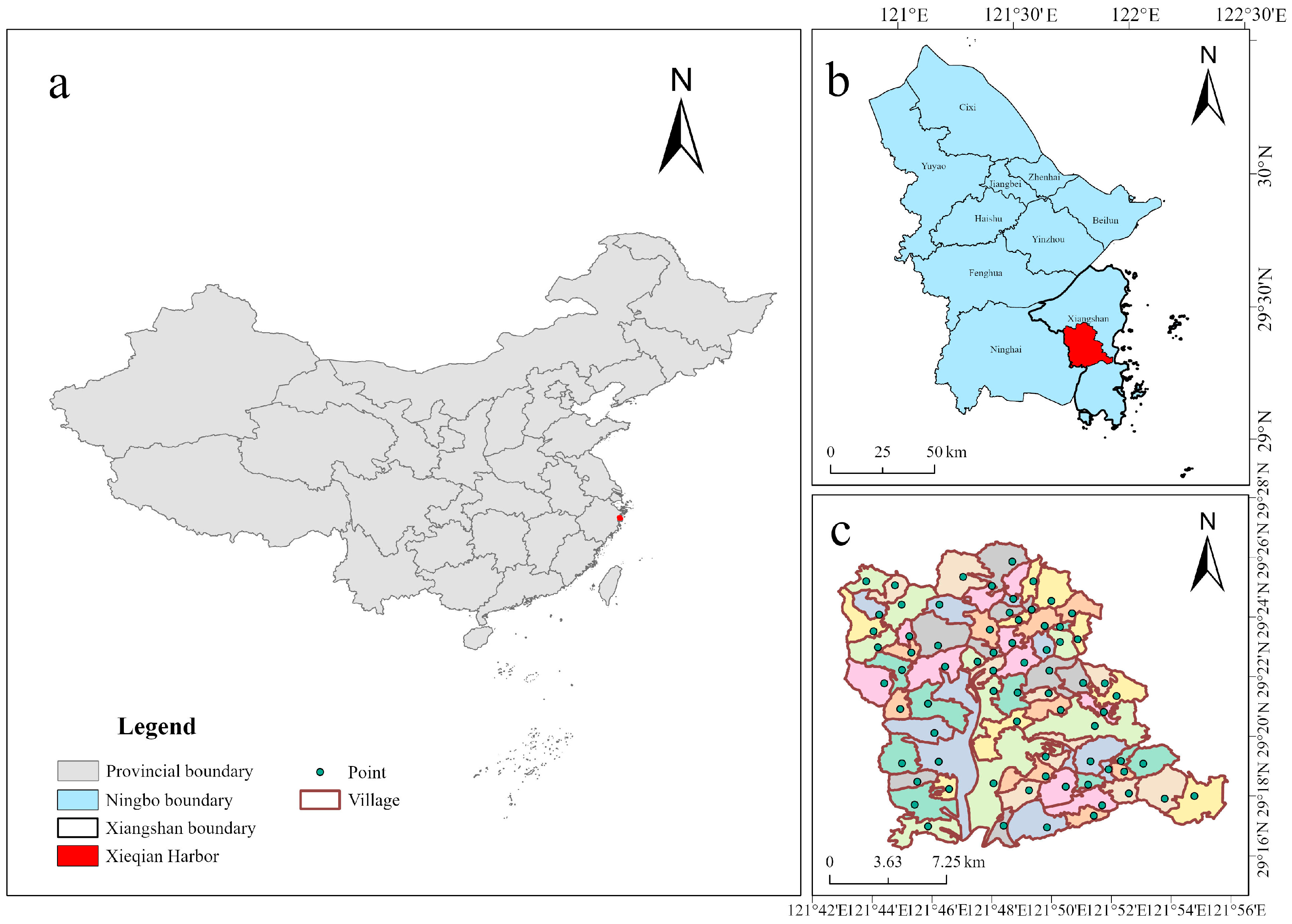
2.1. Study Area

Xieqian Harbor is located in the middle and western part of Xiangshan County, Ningbo City, Zhejiang Province (Figure 1), containing three townships: Sizhoutou Township, Xinqiao Township, and Maoyang Township. It covers a sea area of about 10 km2 and has a total coastline length of 5 km. The area is named because of its resemblance to a crab’s pincer. Surrounded by mountains on three sides and the sea on one side, it has a beautiful ecological environment and distinct coastal features, making it a prime area along Xiangshan’s most scenic coastline. The forest coverage rate of Xieqian Harbor is about 65%, and the air quality excellence rate remains above 90% all year round, making it a natural ecological oxygen bar. In addition, the agriculture, fishery, culture, and tourism industries in Xieqian Harbor are flourishing, and the integration of intangible cultural heritage with the natural landscape enhances the area’s charm and attractiveness. In 2021, the Xieqian Harbor area received 2.64 million tourists, generating a tourism revenue of USD 96 million, and creating over 5000 jobs in ten major categories for the surrounding villages and towns. Xieqian Harbor has outstanding ecological value and great development potential. Local governments in China attach great importance to the ecological protection and sustainable development and utilization of the Xieqian Harbor area and are striving to create a model county-style area.

2.2. Data Sources and Preprocessing

Our study included datasets of administrative boundaries, a digital elevation model (DEM), land use/land cover (LULC), meteorology, and soils (Table 1). The LULC data were sourced from the multi-temporal China National Land Use and Cover Change (CNLUCC) dataset provided by the Resource and Environment Science and Data Center (RESDC), with a spatial resolution of 30 m × 30 m. The dataset was primarily generated through a manual visual interpretation of Landsat TM/ETM satellite imagery. It includes six first-level land use types (cropland, forest land, grassland, water bodies, built-up areas, and unused land) and 25 s-level subcategories. The overall accuracy of the dataset exceeds 90% [39]. This study utilized data from three time points: 2000, 2010, and 2020. Administrative village boundaries were used as the basic unit of analysis and mapping (license number: Zhe Yong S (2020) No. 02); LULC data were used to calculate landscape pattern indices; and the remaining data were used to assess ecological effects. All spatial data were preprocessed using ArcGIS 10.4.1, transformed to the same coordinate system (WGS-84) and spatial resolution (30 m × 30 m).

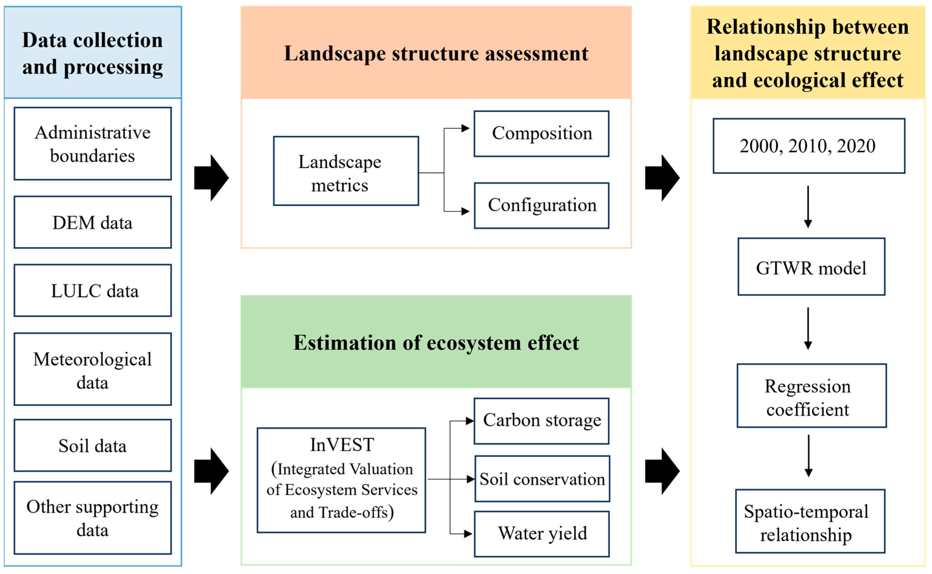
2.3. Research Frameworks

The research framework is shown in Figure 2. First, data were collected and processed to identify 72 administrative village units for mapping and analysis based on administrative village boundary data. An administrative village is an appropriate unit because it is directly associated with many ecological processes [40]. Land use data were then used to calculate landscape indices for Xieqian Harbor in 2000, 2010, and 2020, and ecological effects (carbon storage, soil conservation, and water yield) were assessed using the Integrated Valuation of Ecosystem Services and Trade-offs (InVESTs) model [41,42]. The years 2000, 2010, and 2020 were chosen because the interval of twenty years covers a long time span and facilitates the observation of long-term trends. Meanwhile, these years have complete data, which can reflect the impacts of different development stages and policy implementation on landscape patterns and ecological effects. Finally, spatiotemporal geographically weighted regression (GTWR) models were constructed with the landscape indices as the explanatory variable and ecological effects as dependent variables, respectively, to analyze the impact of changes in landscape patterns on the three typical ecological effects.

2.4. Research Methods

2.4.1. Quantification of Landscape Patterns

The landscape pattern index is an important tool for quantifying landscape composition and configuration. The requirements for selecting metrics are the following: (1) metrics should be closely aligned with the specific objectives of the study and be able to comprehensively characterize the spatial structure of the landscape [43,44]; (2) independent indicators should be selected to improve analytical efficiency and avoid redundancy [45,46,47]; and (3) landscape indices that are easy to interpret and apply should be prioritized to facilitate their application by managers in practical environments [48]. Following these criteria and referring to previous studies [46,49], this study uses a total of eight indices to analyze the landscape characteristics of Xieqian Harbor at the village scale, as follows: the largest patch index (LPI), percentage of landscape (PLAND), patch density (PD), Shannon’s diversity index (SHDI), edge density (ED), area-weighted mean patch shape index (AWMSI), interspersion and juxtaposition index (IJI), and aggregation index (AI). These indices were used to comprehensively describe the spatial structure of the landscape, capturing key aspects such as landscape diversity, spatial heterogeneity, and fragmentation. Notably, the PLAND metrics measure the proportion of a particular land use type within the overall landscape. In Xieqian Harbor, 65% of the land is forested, making it the largest land use type in the region. It occupies a major position in the landscape and has a significant impact on the ecological environment; therefore, we chose forested land as the main representative type, denoted by PLAND_wl. All landscape indices were calculated using Fragstats v4.2.

2.4.2. Estimation of Ecological Effects

According to previous studies [50,51,52], landscape pattern alteration can cause changes in biodiversity, habitat quality, carbon sequestration, water supply, and soil conservation. Meanwhile, previous studies have confirmed that the main ecological benefits of high-intensity land development in the eastern coastal area of Zhejiang that caused significant changes were soil conservation, carbon sequestration, and water production effects [53,54,55]. The potential reason may be that these effects are most susceptible to land use change and have an important role in regional ecosystem stability and regional sustainable development. Therefore, carbon storage, soil conservation, and water yield effects were selected for this study. The data used for each ecological effect estimation session are given in Appendix A. These ecological effects were quantified using Arc GIS spatial analysis tools and the Integrated Valuation of Ecosystem Services and Trade-offs (InVESTs) model.
① Carbon storage (CS)
The InVEST model simulates carbon sequestration by evaluating four carbon pools (aboveground carbon pool, belowground carbon pool, soil carbon pool, and dead organic carbon pool). Users provide spatial data on land use and carbon density tables to estimate carbon stocks [24], which are calculated using the following formula:
C t o t a l = C a b o v e + C b e l o w + C s o i l + C d e a d
where C t o t a l is the total carbon stock of the region; C a b o v e is the carbon density of the aboveground part; C b e l o w is the carbon density of the belowground part; C s o i l is the soil carbon density; and C d e a d is the dead carbon density. Based on this, the input data for the carbon storage module are mainly land use and biophysical table data.
② Soil Conservation (SC)
Soil conservation service, as an important ecosystem regulation, is essential to prevent regional land degradation and reduce flood risk. It refers to the ecosystem’s ability to prevent soil loss through erosion and to retain sediments. The InVEST model usually uses the Revised Universal Soil Loss Equation (RUSLE) to estimate the average annual soil loss due to erosion in different regions [56]. RUSLE takes into account factors such as rainfall erosivity, soil erodibility, and topographic slope. The calculation formula is as follows:
R U S L E x = R x × K x × L S x × C x × P x
where R U S L E x is the soil erosion of raster x; R x is the rainfall erosion factor; K x is the soil erodibility factor; L S x is the topographic factor (slope length and steepness); C x is the vegetation cover factor; and P x is the empirical factor. Based on this, this study requires the input of raster data for land use, DEM, the rainfall erosion factor, and the soil erodibility factor, as well as surface vector data and a biophysical table for the Xieqian Harbor watershed. Additionally, inputs include Kb, Maximum SDR Value, I C0, and the Maximum L Value, which are taken from the recommended values in the model’s instruction manual.
③ Water Yield (WY)
The annual water yield module in the InVEST model was used to calculate the water supply of the ecosystem. This module is based on the water cycle process, assuming that the water production of the raster cells is all pooled to the outlet of the watershed by means of surface runoff or subsurface runoff. The water production is approximated to be equal to the difference between precipitation and evapotranspiration from the surface and vegetation [57], which was calculated using the following formula:
Y x = 1 E a , x P x × P x
where Y x is the water production of raster x; E a , x is the average annual evapotranspiration; and P x is the average annual precipitation. Based on this, the operation of the water supply module requires the input of raster data on land use, precipitation, and evapotranspiration, as well as watershed surface vector data and biophysical tables. Finally, the model results are calibrated by adjusting the seasonal parameter, Z.

2.4.3. Geographically and Temporally Weighted Regression Model (GTWR)

The geographically and temporally weighted regression (GTWR) model is a spatial statistical model that extends the geographically weighted regression (GWR) by incorporating the temporal dimension. It fully reflects the temporal changes in variable data while revealing the heterogeneity of the variables in both time and space, thereby better explaining the spatiotemporal relationships between independent and dependent variables [24,58,59,60]. In this paper, the GTWR model is used to explore the spatiotemporal characteristics of landscape indices and ecological effects. The calculation formula is the following:
Y i = β 0 x i , y i , t i + k = 1 β k x i , y i , t i X i k + ε i
where Y i is the ecological effect value of the i-th administrative village; x i , y i , t i are the longitude, latitude, and time of the i-th administrative village, respectively; β 0 x i , y i , t i is the regression intercept of the i-th administrative village; β k x i , y i , t i is the regression coefficient of the k-th landscape variable in the i-th administrative village; X i k is the value of the k-th landscape index in the i-th administrative village; and ε i is the model residual. In this study, the correlation and multicollinearity between landscape variables and ecological effects were tested to ensure that all selected landscape variables (independent variables) were statistically significant in relation to ecological effects (dependent variables) and exhibited no multicollinearity. The GTWR model calculations were primarily conducted using ArcGIS 10.4.1 software with the GTWR plugin developed by Huang et al. [24].

3. Results

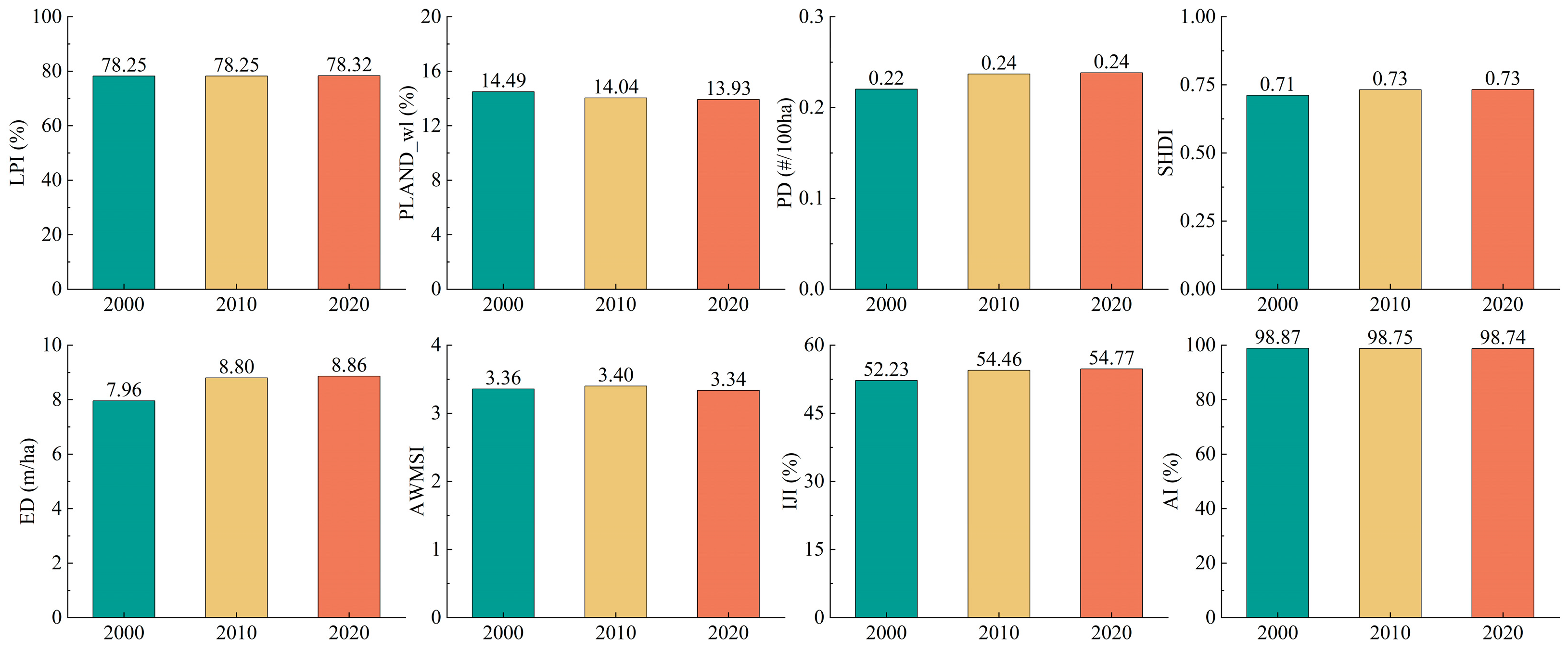
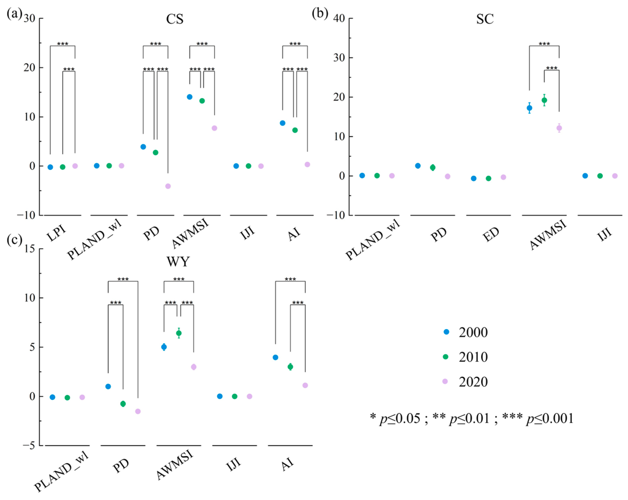
3.1. Changes in Landscape Patterns from 2000 to 2020

Eight landscape pattern indices were selected to explore the landscape pattern changes in Xieqian Harbor from 2000 to 2020. As can be seen in Figure 3, in terms of landscape area and number at the village scale, from 2000 to 2020, the patch density (PD) of Xieqian Harbor increased gradually, with a growth rate of 9.09%, indicating that the degree of fragmentation of landscape patches within the study area deepened, and the landscape heterogeneity was increasing. In terms of landscape shape, the edge density index (ED) continued to grow, increasing by 11.31% from 2000 to 2020, with an increasing degree of irregularity and overall boundary complexity at the landscape level. The area-weighted mean patch shape index (AWMSI) of Xieqian Harbor increased slightly from 2000 to 2010 and then decreased from 2010 to 2020. This indicated that the landscape became more irregular in shape during the first decade, suggesting increased fragmentation, but then transitioned to a more simplified structure in the following decade. In terms of landscape diversity, Shannon’s diversity index (SHDI) showed a growth rate of 2.82%, indicating that the landscape patches of Xieqian Harbor increased in amplitude and landscape types became more diverse. In terms of landscape aggregation, the interspersion and juxtaposition index (IJI) showed an overall increasing trend with a growth rate of 4.86%, reflecting that the ratio of neighboring patch types in the study area was increasing, and the tightness between the same patches was decreasing. The aggregation index (AI) continued to decrease, indicating that the regional landscape fragmentation was increasing, and the aggregation of landscape patches, as well as the controlling role of dominant landscape types, was decreasing.

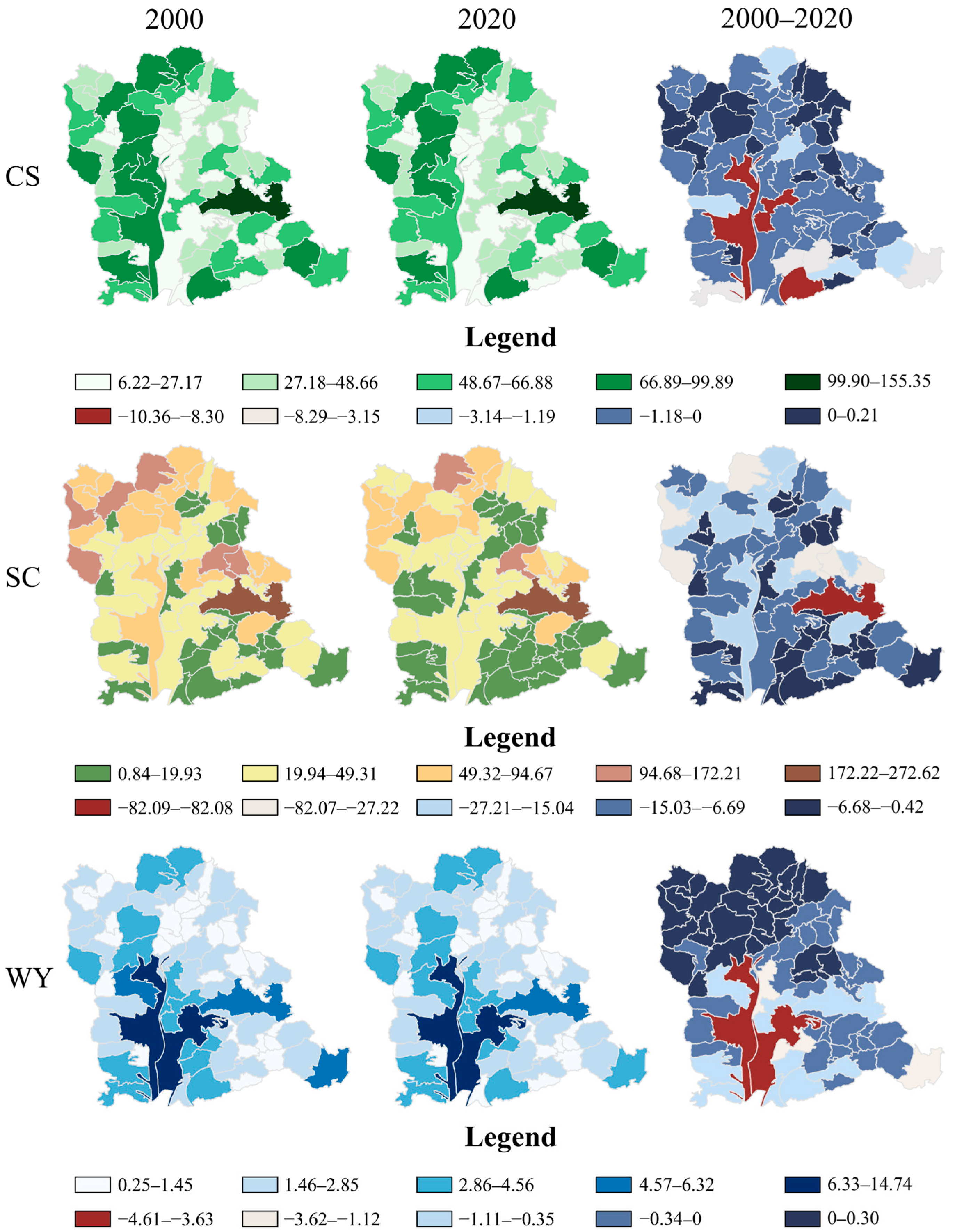
3.2. Changes in Ecological Effects from 2000 to 2020

Table 2 showed the carbon storage, soil conservation, and water yield in Xieqian Harbor from 2000 to 2020, along with their rates of change. The results indicated that by 2020, the carbon storage, soil conservation, and water yield of Xieqian Harbor were 31.47 million tons, 2.34 billion tons, and 153 million cubic meters, respectively. Over the past 20 years, there have been significant declines in these three ecological effects, with carbon storage decreasing by 572.6 thousand tons (−1.79%), soil conservation by 853 million tons (−26.75%), and water yield by 19 million cubic meters (−11.19%).
Figure 4 showed the distribution and changes in carbon storage, soil conservation, and water yield in each administrative village of Xieqian Harbor from 2000 to 2020. The results indicated significant spatial heterogeneity in these three ecological effects. The administrative village with the highest carbon stock and soil retention was Dongxi Village, with higher areas mainly distributed in woodlands with high forest cover. The administrative village with the highest water yield was Chongtu Village, with higher areas mainly concentrated in the southern estuary. From 2000 to 2020, there was a significant decrease in carbon storage in the southern townships of Xieqian Harbor; soil conservation showed significant spatial distribution changes, with Dongxi Village experiencing the largest decrease; and water yield significantly decreased in the southern townships, while the northwestern townships showed a significant increase.

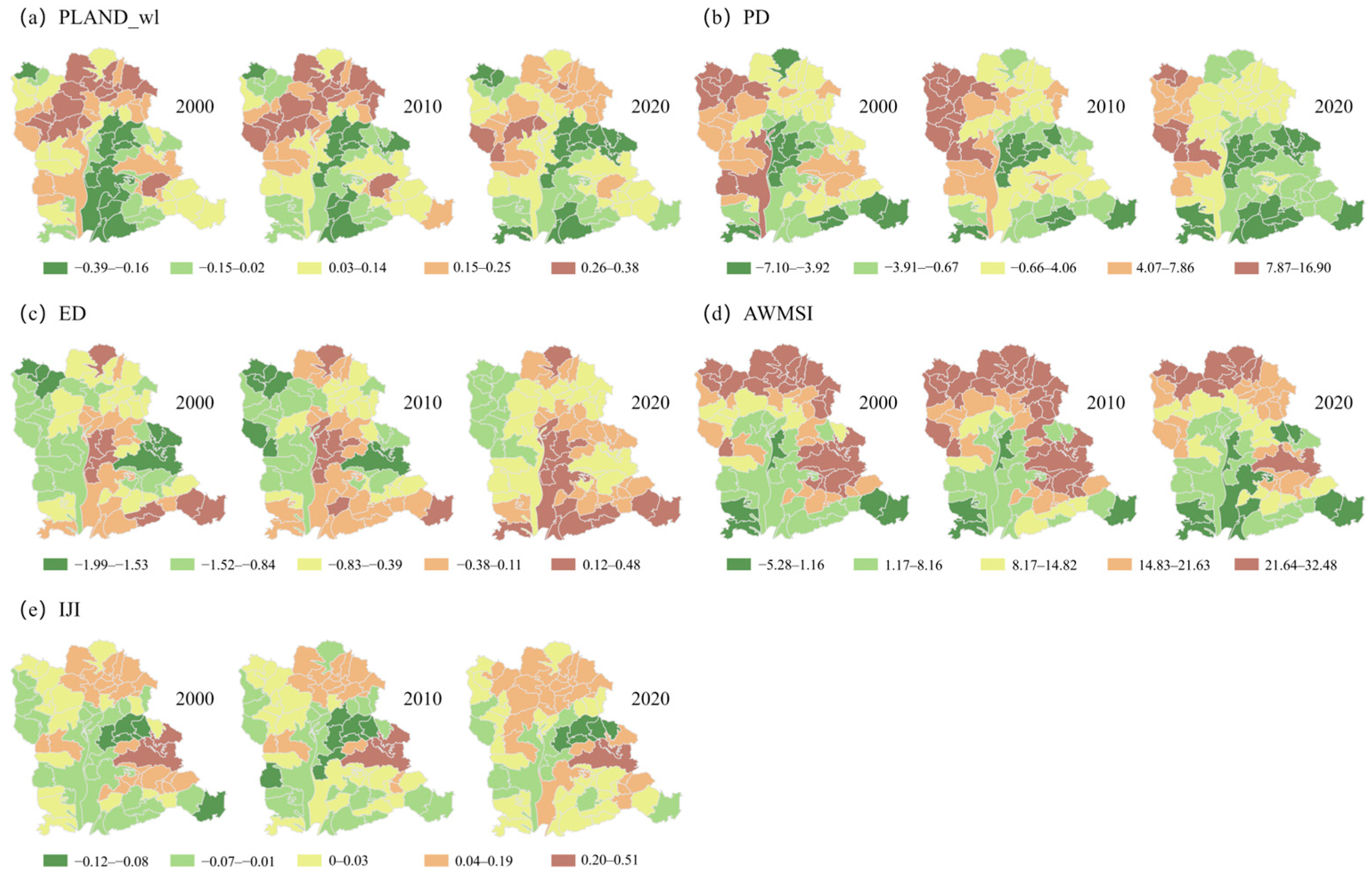
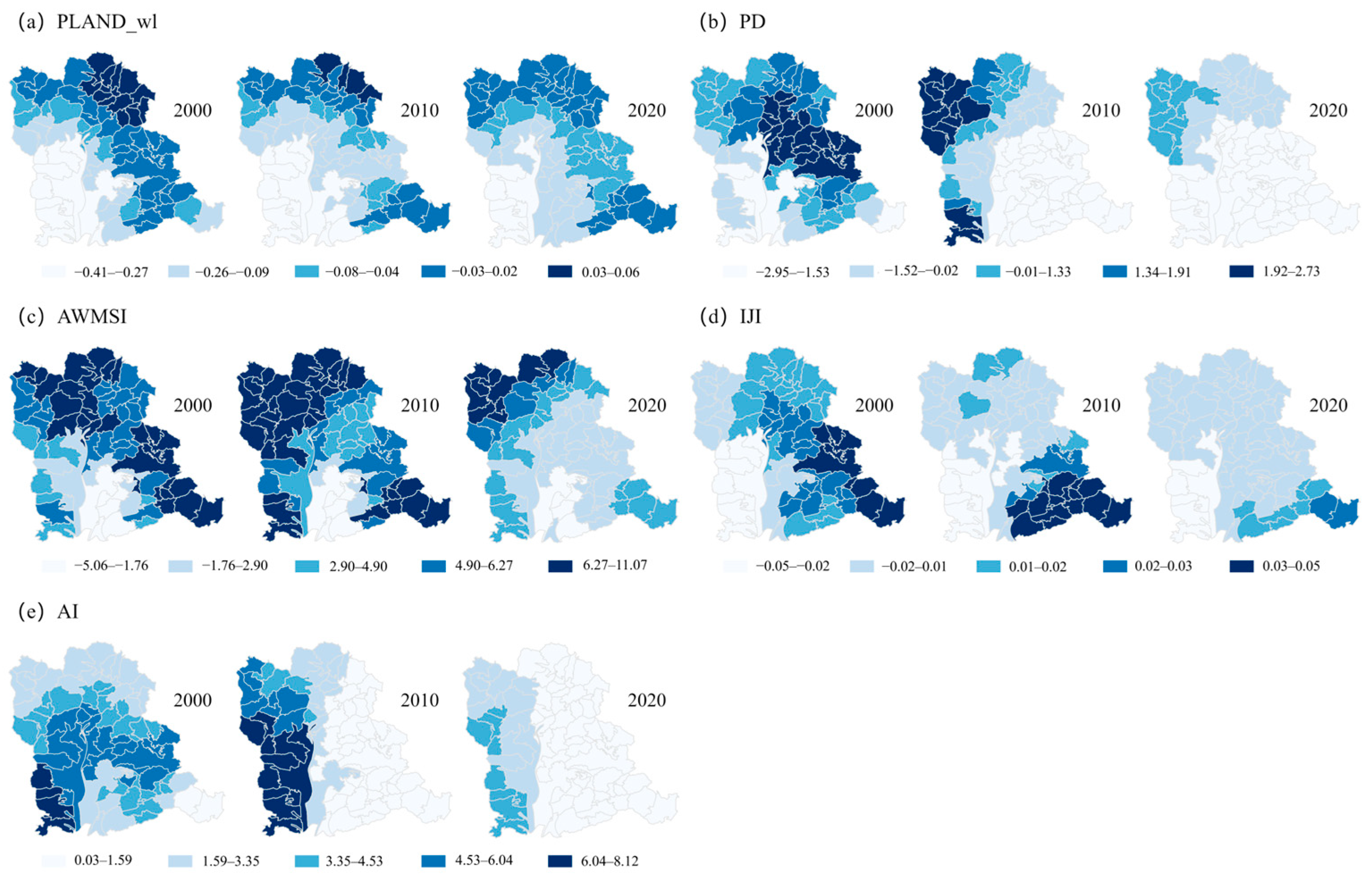
3.3. Spatiotemporal Relationships Between Landscape Structure and Ecological Effects

3.3.1. Variable Selection

The results showed that six landscape indices were used to predict CS, namely the largest patch index (LPI), percentage of landscape for forest land (PLAND_wl), patch density (PD), area-weighted mean patch shape index (AWMSI), interspersion and juxtaposition index (IJI), and aggregation index (AI); five were used to predict SC, namely the percentage of landscape for forest land (PLAND_wl), patch density (PD), edge density (ED), area-weighted mean patch shape index (AWMSI), and interspersion and juxtaposition index (IJI); and five were used to predict WY, namely the percentage of landscape for forest land (PLAND_wl), patch density (PD), area-weighted mean patch shape index (AWMSI), interspersion and juxtaposition index (IJI), and aggregation index (AI) (see Appendix A Figure A1 and Table A3 for details). These indices demonstrated strong explanatory power in the GTWR model, with R2 values of 0.72, 0.83, and 0.86 for CS, SC, and WY, respectively.

3.3.2. Spatiotemporal Change Analysis

The results of the GTWR regression coefficients based on landscape variables and ecological effects are shown in Figure 5. The signs of the regression coefficients indicated that landscape variables have both positive and negative effects on ecological effects. Additionally, the effects of the same landscape variables on different ecological effects were different. Specifically, the average coefficients of PD for the three ecological effects (CS, SC, and WY) were 0.87, 1.52, and −0.42, respectively; and the average coefficients of IJI for the ecological effects were 0.01, 0.07, and 0.01, respectively. It was particularly important to note that AWMSI contributed the most to the ecological effects because its regression coefficients had the largest absolute values overall. Furthermore, the impact of landscape variables on ecological effects varied over time. For example, the average regression coefficients of PD with CS in 2000, 2010, and 2020 were 3.92, 2.76, and −4.08, respectively, with significant differences between years. AWMSI with CS, AI with CS, and AWMSI with WY showed similar results.
By plotting the temporal and spatial distribution patterns of the relationships between landscape variables and CS, SC, and WY in 2000, 2010, and 2020, it was found that the effects of landscape variables on ecology were complex in both temporal and spatial dimensions. PLAND_wl, AWMSI, and AI mainly showed positive effects on carbon stocks, with their coefficient means being 0.07, 11.67, and 5.46, respectively. As the time advanced, the mean value of the regression coefficient of LPI gradually increased, while the mean value of the coefficients of PD, AWMSI, and AI gradually decreased, indicating that the negative effect of the largest patches was enhanced, and the positive effects of patch density, landscape shape, and aggregation were decreased. This suggested that a landscape pattern with reduced patch fragmentation and larger and more aggregated patches was beneficial for increasing carbon sequestration.
In terms of impact stability, PLAND_wl maintained a relatively stable impact from 2000 to 2020, with the coefficients showing a gradual decrease from northwest to southeast. Other landscape variables fluctuated considerably over time, with the trend in the first decade reversing in the second. For example, many dark green areas in PD in 2010 were replaced by light green and yellowish areas in 2020. Similar changes could be observed for IJI (Figure 6).
Spatially, the high mean values of the landscape variables, except for PD, were mainly distributed in the northern part of Xieqian Harbor, a mountainous area with a concentration of forested land. Additionally, the regression coefficients between landscape variables and SC fluctuated less over time compared to carbon sequestration (Figure 7). PLAND_wl and PD had predominantly negative effects on water production from 2000 to 2020, while AWMSI, IJI, and AI had broader positive effects (Figure 8). The heterogeneity in the distribution of regression coefficients increased over time, with the emergence of small, scattered, and independent clusters.

4. Discussion

Our study found that patch density (PD), Shannon’s diversity index (SHDI), edge density (ED), and the interspersion and juxtaposition index (IJI) increased while the aggregation index (AI) decreased in Xieqian Harbor from 2000 to 2020; and that carbon storage, soil conservation, and water yield decreased by 572.6 thousand tons, 853 million tons, and 19 million cubic meters, respectively. This revealed an increase in landscape fragmentation and a gradual deterioration of the ecosystem in Xieqian Harbor. This was consistent with the results of Li and Cui’s study [61,62], which found that the replacement of large tracts of cropland and forest land by construction land for urban development not only destroys the existing landscape structure but also greatly weakens the ecological effect, including a reduction in biodiversity, decreased carbon sequestration capacity, diminished soil retention, degradation of water quality, and reduced ecosystem stability. Meanwhile, our study also found that the high-value areas of CS, SC, and WY increments were mainly distributed in administrative villages with high vegetation cover, which further proved the great ecological value of forest resources.
Previous studies have mostly analyzed the relationship between landscape variables and ecological effects through statistical models such as Ordinary Least Squares (OLS) regression, Geographically Weighted Regression (GWR), and Moran’s I [63,64,65]. These models have provided valuable insights into spatial patterns, but they often assume static relationships and fail to capture spatiotemporal heterogeneity. In contrast, the geographically and temporally weighted regression (GTWR) model extends the analytical framework by incorporating both spatial and temporal variations, making it more suitable for dynamic landscape–ecological interactions [66]. First, the model can accurately calculate the regression coefficient of a landscape variable on a specific ecological effect at any time and spatial location. Second, it can further identify and determine the key landscape variables that affect ecological effects, providing an important basis for management and optimization. Finally, by analyzing the dynamic changes in impact over time, the GTWR model can assess the instability of this change, thereby measuring the reliability of the information obtained to support decision-making. These functions provide a scientific basis for improving current landscape management and help promote the positive development and sustainable use of ecosystem services.
This study uses the GTWR model to analyze the dynamic changes in regression coefficients and reveal the complex spatiotemporal interactions between landscape variables and ecological effects. It was found that the relationship becomes very complex when temporal non-stationarity and spatial heterogeneity are combined. First, a landscape variable was positively correlated with one ecological effect and negatively correlated with another ecological effect at the same moment. For example, PLAND_wl in Xieqian Harbor in 2000 was positively associated with CS and SC and negatively associated with WY; the same results were observed in 2010 and 2020. Xieqian Harbor was surrounded by mountains on three sides, and 65% of the land was forested, which effectively stored carbon through above- and below-ground biomass accumulation. The complex root system helped to maintain soil structure and stability, thus improving soil retention; however, dense forests, with strong evapotranspiration, draw a large amount of water from the soil, which reduces surface runoff [67,68] and lowers the amount of water production. Similar research has been verified in other regions. For example, Liu et al. found that landscape configuration in the Yellow River Basin has a positive effect on carbon sequestration and a negative effect on water production [69]. This finding had important implications for ecological management and decision-making in Xieqian Harbor. Managers had to comprehensively consider the interactions between different ecological effects, balance ecological functions, and mitigate potential drawbacks in order to achieve more sustainable ecosystem management.
We found that the area-weighted mean patch shape index (AWMSI) was the most critical factor affecting the ecological function of Xieqian Harbor. The AWMSI measured the degree of irregularity of patch shape in the landscape, with larger values indicating more irregular and complex patches. Complex patch shapes formed a variety of edges and many microhabitats, which enhanced the edge effect and promoted ecological interactions among species [70]. For example, Li et al.’s study on the middle and lower reaches of Yangtze River found that wetland patch shape complexity was significantly correlated with ecological value [71]; and Wang and Vallarino’s study on coastal areas found that landscape shape complexity promoted water retention capacity [72,73]. All these studies emphasized that in coastal areas, complex landscape shapes support ecological functioning. Xieqian Harbor was located in the eastern coast of Zhejiang, with a meandering coastline and complex landscapes of rivers, harbors, and shallow wetlands, which helped to form diverse microhabitats, improved carbon sequestration, and promoted soil retention and the stability of the ecosystem.
Our results revealed significant temporal instability in the response of most landscape pattern indices to changes in carbon stocks. This instability is attributed to the combined effects of the inherent processes of carbon storage formation (such as plant growth and soil carbon decomposition), natural disturbances (such as typhoons and fires), and human activities [74,75]. As a typical inner harbor area, the ecology of Xieqian Harbor was vulnerable to natural disasters such as typhoons and landslides. In addition, anthropogenic land use changes could also rapidly alter the current status of vegetation cover, directly leading to drastic changes in carbon stocks, thus reflecting the fluctuation of regression coefficients over time. In contrast, the more stable effects of landscape change on soil retention and water production may have been due to the fact that these services depend on more stable landscape characteristics such as physical attributes like soil type, soil texture, and geomorphology, which changed relatively slowly over time. This was also demonstrated in a similar study by Li et al. in Yan’an [76]. This demonstrates the need for adaptive management decisions that considered the temporal dynamics of landscape patterns and their impacts on ecological functioning, especially in terms of carbon sinks.
Over time, our study found an increase in the heterogeneity of the distribution of regression coefficients between some landscape variables and ecological effects, forming scattered, independent clusters, such as the aggregation index (AI) and carbon storage (CS), percentage of landscape for forest land (PLAND_wl) and soil conservation (SC), and interspersion and juxtaposition index (IJI) and water yield (WY) (Figure 6f, Figure 7a, and Figure 8d). This indicates that the impact of certain landscape variables on ecological effects has become more complex and diverse. The spatial heterogeneity observed in the regression coefficient distribution maps could be attributed to the uneven distribution of landscape and ecological functions. Similar patterns were found in the study by Ran et al., who noted that changes in land use result in significant regional and temporal variations in the impact of landscape on ecosystem services, such as water yield [77].
In the Xieqian Harbor area, our study utilized a finer administrative village-level scale to more comprehensively capture the local characteristics and relationships between landscape structure and ecological effects, incorporating the temporal dimension for multidimensional analysis and understanding. Firstly, village-level research enabled the examination of how specific landscape variables affected ecological effects within an individual administrative village, revealing subtle spatial heterogeneity and avoiding generalizations and errors that might occur at a macro scale [78,79]. Second, analyzing at the village scale helped identify key landscape variables affecting ecological effects in a given region and period for dynamic monitoring and assessment. Third, land use and management needs varied across administrative villages, and village-scale studies could provide more specific ecological management recommendations for local governments and communities. For example, Gao’s specific landscape restructuring for an administrative village in the Yangtze River Delta directly improved the ecological effects of the village. This kind of fine-tuned management helped improve resource utilization efficiency and enhance ecosystem stability and resilience [80]. Finally, by studying the relationship between landscape and ecological effects at the village scale, the impacts of future landscape changes on ecosystem services could be better understood and predicted. This was crucial for the development of long-term sustainable development policies and planning to ensure the positive continuation of ecological effects.

5. Conclusions

Human activities in inner harbor regions have driven landscape changes that directly lead to the degradation of key ecological functions. Our study, conducted at the village level, utilized the GTWR model along with eight landscape indices and three typical ecological effects to quantify the spatiotemporal variations in the relationship between landscape structure and ecological effects in Xieqian Harbor from 2000 to 2020. The results revealed that over the past 20 years, the complexity, heterogeneity, and diversity of landscape patches in Xieqian Harbor have increased, while carbon sequestration, soil retention, and water yield capacities have steadily declined. The interplay of temporal non-stationarity and spatial heterogeneity made the relationship between landscape patterns and ecological effects highly complex. On the one hand, a single landscape variable might enhance one ecological effect while diminishing another, necessitating a balanced approach in landscape management that carefully considers trade-offs among different ecological objectives. On the other hand, over the past two decades, all regression coefficients showed varying degrees of change, with numerous small, dispersed, and independent clusters emerging in the distribution maps. We also found that carbon sequestration exhibited higher temporal instability in response to landscape variables compared to the other two ecological effects, indicating a need for special attention. The area-weighted mean patch shape index (AWMSI) was identified as a key factor influencing the three ecological effects in Xieqian Harbor. The successful application of the GTWR model in this study underscores the potential of spatiotemporal methods in analyzing the relationship between landscape patterns and ecological effects. The results highlight the advantages of village-scale analysis in capturing the localized impacts of landscape changes on ecological effects, which may not be as evident in larger-scale studies. These findings provide critical insights for developing targeted ecological management strategies and sustainable development policies. Nevertheless, this study is constrained by the use of land-use data from discrete time points. Future research should integrate more continuous datasets to better capture temporal dynamics and expand the analysis to broader regions, thereby offering more comprehensive guidance for sustainable landscape management.

Author Contributions

Conceptualization, X.Y. and J.L.; methodology, Q.P., S.L., and M.X.; writing—original draft preparation, Q.P. and S.L.; writing—review and editing, X.Y., J.L., and M.X.; visualization, Q.P. and S.L.; supervision, X.Y. and M.X.; project administration, X.Y.; funding acquisition, X.Y. and J.L. All authors have read and agreed to the published version of the manuscript.

Funding

This work was supported by the National Natural Science Foundation of China (Grant No. 42371027), and the Key Technology Breakthrough Plan Project of Science and Innovation Yongjiang 2035 (Grant No. 2022Z181, 2023Z146, 2024Z249, 2024Z262).

Data Availability Statement

All data utilized in this study are derived from publicly available sources, including the Resource and Environment Science and Data Center, the Geospatial Data Cloud, and the Harmonized World Soil Database v1.2. These data can be found here: [http://www.resdc.cn; http://www.gscloud.cn; https://gaez.fao.org/pages/hwsd, (accessed on 27 January 2024)]. Additional experience-based values and methodological details are provided in Appendix A for further reference.

Conflicts of Interest

The authors declare no conflicts of interest.

Appendix A

Table A1. Landscape pattern indices.
MetricsAbbreviation (Scale)Annotation
(1) Area and Quantity
Largest Patch IndexLPI (Landscape and Class)This index expresses the proportion of the largest patch area in a specific landscape type to the total landscape area of the whole region (0 < LPI < 100); if the maximum patch area in a given landscape type gradually shrinks, the LPI tends to 0, whereas if it gradually expands and finally occupies the whole region, the LPI is close to 100 [81,82].
Percentage of LandscapePLAND (Class)This index is used to quantify the proportion of the abundance of a particular landscape patch category to that of the regional overall landscape (0 < PLAND < 100) [83].
Patch DensityPD (Class)This index is used to quantify the number of patches of a particular landscape patch category per unit area of the regional overall landscape (0 < PD < ∞). This index provides insight into the fragmentation and spatial distribution of landscape patches, with higher values indicating greater fragmentation and a more heterogeneous landscape structure [84,85].
(2) Shape and Edge
Edge DensityED (Landscape and Class)This index reflects the length of the edges per unit area [86].
Area-Weighted Mean Patch Shape IndexAWMSI (Class)This index is used to quantify the complexity of the shape of landscape patches, taking into account the size of each patch. This index provides insight into the geometric complexity and irregularity of patch shapes within a landscape, with higher values indicating more complex shapes [87].
(3) Landscape Diversity
Shannon’s Diversity IndexSHDI (Landscape)This index is based on the general knowledge that the degree of regional land exploitation is proportional to that of land diversification; the higher the index, the higher the degree of regional land exploitation and development [88,89,90].
(4) Spatial Distribution
Interspersion and Juxtaposition IndexIJI (Landscape and Class)This metric is applied to reflect the distribution of patch adjacency, isolating the interspersion or intermixing of landscape patches (0 < IJI < 100); IJI is close to 0 if the patch is adjacent to only one other patch, whereas it is close to 100 if the patch is equally adjacent to all other patches [43,91].
Aggregation IndexAI (Class)This index is performed from the adjacency matrix, reflecting the frequency of different landscape patch types occurring side-by-side in a regional landscape (including adjacencies for the same landscape type) (0 ≤ AI ≤ 100); it increases as the focal patch type is increasingly aggregated and tends to 100 when the patch type is maximally aggregated into a single and compact patch [92].
Table A2. Data types and sources for the three ecological effects.
Input DataData Source
Carbon storageLULCResource and Environment Science and Data Center (http://www.resdc.cn/)
Carbon poolsReference to the relevant literature [55]
Soil conservationDEMGeospatial data cloud (http://www.gscloud.cn/)
PrecipitationResource and Environment Science and Data Center (http://www.resdc.cn/)
Root depth, soil texture, and organic contentHarmonized World Soil Database v 1.2 (https://gaez.fao.org/pages/hwsd)
LULCResource and Environment Science and Data Center (http://www.resdc.cn/)
Biophysical tableReference to the relevant literature [93]
WatershedsResource and Environment Science and Data Center (http://www.resdc.cn/)
Water yieldPrecipitationResource and Environment Science and Data Center (http://www.resdc.cn/)
Potential evapotranspirationResource and Environment Science and Data Center (http://www.resdc.cn/)
Root-restricting layer depth(http://globalchange.bnu.edu.cn/research/cdtb.jsp, accessed on 7 January 2025)
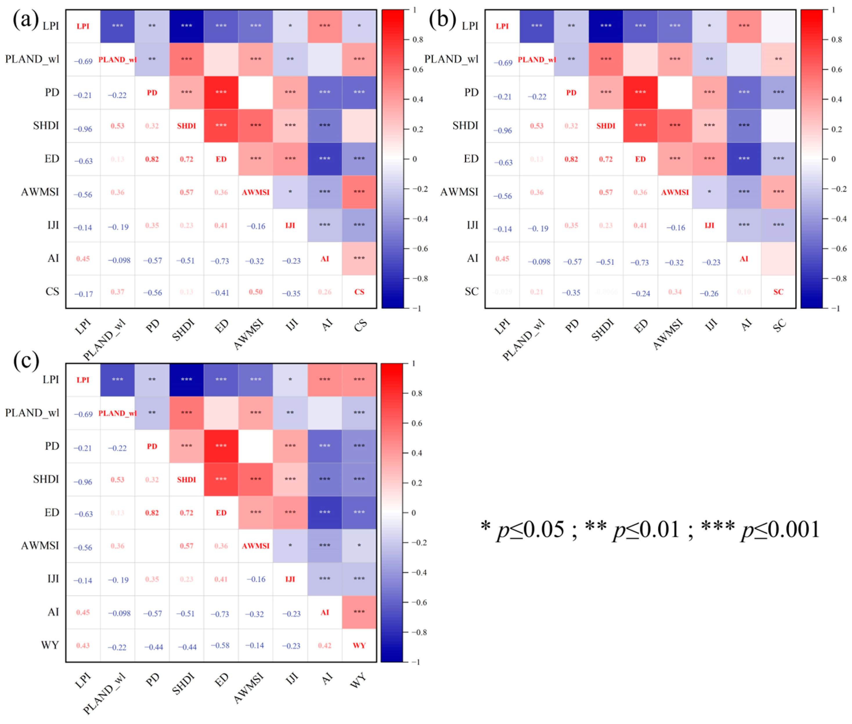
Figure A1. Pearson’s test for landscape variables and ecological effects. (a) CS, (b) SC, (c) WY.
Land 14 00319 g0a1
Table A3. Multicollinearity test of selected landscape variables and ecological effects.
LPIPLAND_wlPDSHDIEDAWMSIIJIAI
VIFVIFVIFVIFVIFVIFVIFVIF
CS6.2503.0347.263NA14.7241.9451.6132.189
SCNA1.6926.198NA8.0371.8841.592NA
WY34.2184.1327.28225.83414.7262.0651.6622.195
Notes: NA denotes that the metric is not used as an explanatory variable.

References

  1. Hein, C. Port Cities and Urban Waterfronts: How Localized Planning Ignores Water as a Connector. WIREs Water 2016, 3, 419–438. [Google Scholar] [CrossRef]
  2. Huang, B.; Ouyang, Z.; Zheng, H.; Zhang, H.; Wang, X. Construction of an Eco-Island: A Case Study of Chongming Island, China. Ocean Coast. Manag. 2008, 51, 575–588. [Google Scholar] [CrossRef]
  3. Sharma, D.; Rao, K.; Ramanathan, A.L. A Systematic Review on the Impact of Urbanization and Industrialization on Indian Coastal Mangrove Ecosystem. In Coastal Ecosystems; Madhav, S., Nazneen, S., Singh, P., Eds.; Coastal Research Library; Springer International Publishing: Cham, Switzerland, 2022; Volume 38, pp. 175–199. ISBN 978-3-030-84254-3. [Google Scholar]
  4. Sempere-Valverde, J.; Guerra-García, J.M.; García-Gómez, J.C.; Espinosa, F. Coastal Urbanization, an Issue for Marine Conservation. In Coastal Habitat Conservation; Elsevier: Amsterdam, The Netherlands, 2023; pp. 41–79. [Google Scholar]
  5. Bao, J.; Gao, S. Long-Term Reclamation of Tidal Flats of Chongming Island and Ecological Security of Yangtze Estuary, China. Reg. Environ. Change 2024, 24, 74. [Google Scholar] [CrossRef]
  6. Cao, W.; Li, R.; Chi, X.; Chen, N.; Chen, J.; Zhang, H.; Zhang, F. Island Urbanization and Its Ecological Consequences: A Case Study in the Zhoushan Island, East China. Ecol. Indic. 2017, 76, 1–14. [Google Scholar] [CrossRef]
  7. Latimer, J.S.; Boothman, W.S.; Pesch, C.E.; Chmura, G.L.; Pospelova, V.; Jayaraman, S. Environmental Stress and Recovery: The Geochemical Record of Human Disturbance in New Bedford Harbor and Apponagansett Bay, Massachusetts (USA). Sci. Total Environ. 2003, 313, 153–176. [Google Scholar] [CrossRef] [PubMed]
  8. Chapin, F.S.; Carpenter, S.R.; Kofinas, G.P.; Folke, C.; Abel, N.; Clark, W.C.; Olsson, P.; Smith, D.M.S.; Walker, B.; Young, O.R. Ecosystem Stewardship: Sustainability Strategies for a Rapidly Changing Planet. Trends Ecol. Evol. 2010, 25, 241–249. [Google Scholar] [CrossRef]
  9. Turner, W.R.; Brandon, K.; Brooks, T.M.; Costanza, R.; Da Fonseca, G.A.; Portela, R. Global Conservation of Biodiversity and Ecosystem Services. BioScience 2007, 57, 868–873. [Google Scholar] [CrossRef]
  10. Wu, M.; Liu, Y.; Xu, Z.; Yan, G.; Ma, M.; Zhou, S.; Qian, Y. Spatio-Temporal Dynamics of China’s Ecological Civilization Progress after Implementing National Conservation Strategy. J. Clean. Prod. 2021, 285, 124886. [Google Scholar] [CrossRef]
  11. Chi, Y.; Shi, H.; Zheng, W.; Wang, E. Archipelagic Landscape Patterns and Their Ecological Effects in Multiple Scales. Ocean Coast. Manag. 2018, 152, 120–134. [Google Scholar] [CrossRef]
  12. Zhao, X.; Huang, G. Urban Watershed Ecosystem Health Assessment and Ecological Management Zoning Based on Landscape Pattern and SWMM Simulation: A Case Study of Yangmei River Basin. Environ. Impact Assess. Rev. 2022, 95, 106794. [Google Scholar] [CrossRef]
  13. Song, S.; Yu, D.; Li, X. Impacts of Changes in Climate and Landscape Pattern on Soil Conservation Services in a Dryland Landscape. Catena 2023, 222, 106869. [Google Scholar] [CrossRef]
  14. Deng, G.; Jiang, H.; Zhu, S.; Wen, Y.; He, C.; Wang, X.; Sheng, L.; Guo, Y.; Cao, Y. Projecting the Response of Ecological Risk to Land Use/Land Cover Change in Ecologically Fragile Regions. Sci. Total Environ. 2024, 914, 169908. [Google Scholar] [CrossRef] [PubMed]
  15. Qiao, J.; Deng, L.; Liu, H.; Wang, Z. Spatiotemporal Heterogeneity in Ecosystem Service Trade-Offs and Their Drivers in the Huang-Huai-Hai Plain, China. Landsc. Ecol. 2024, 39, 42. [Google Scholar] [CrossRef]
  16. Hu, J.; Zhang, J.; Li, Y. Exploring the Spatial and Temporal Driving Mechanisms of Landscape Patterns on Habitat Quality in a City Undergoing Rapid Urbanization Based on GTWR and MGWR: The Case of Nanjing, China. Ecol. Indic. 2022, 143, 109333. [Google Scholar] [CrossRef]
  17. Smith, P.; Adams, J.; Beerling, D.J.; Beringer, T.; Calvin, K.V.; Fuss, S.; Griscom, B.; Hagemann, N.; Kammann, C.; Kraxner, F.; et al. Land-Management Options for Greenhouse Gas Removal and Their Impacts on Ecosystem Services and the Sustainable Development Goals. Annu. Rev. Environ. Resour. 2019, 44, 255–286. [Google Scholar] [CrossRef]
  18. Marini, L.; Ayres, M.P.; Jactel, H. Impact of Stand and Landscape Management on Forest Pest Damage. Annu. Rev. Entomol. 2022, 67, 181–199. [Google Scholar] [CrossRef] [PubMed]
  19. Ma, S.; Deng, G.; Wang, L.-J.; Hu, H.; Fang, X.; Jiang, J. Telecoupling between Urban Expansion and Forest Ecosystem Service Loss through Cultivated Land Displacement: A Case Study of Zhejiang Province, China. J. Environ. Manag. 2024, 357, 120695. [Google Scholar] [CrossRef]
  20. Tu, D.; Cai, Y.; Liu, M. Coupling Coordination Analysis and Spatiotemporal Heterogeneity between Ecosystem Services and New-Type Urbanization: A Case Study of the Yangtze River Economic Belt in China. Ecol. Indic. 2023, 154, 110535. [Google Scholar] [CrossRef]
  21. Zheng, L.; Wang, Y.; Li, J. Quantifying the Spatial Impact of Landscape Fragmentation on Habitat Quality: A Multi-Temporal Dimensional Comparison between the Yangtze River Economic Belt and Yellow River Basin of China. Land Use Policy 2023, 125, 106463. [Google Scholar] [CrossRef]
  22. Liu, S.; Wang, Z.; Wu, W.; Yu, L. Effects of Landscape Pattern Change on Ecosystem Services and Its Interactions in Karst Cities: A Case Study of Guiyang City in China. Ecol. Indic. 2022, 145, 109646. [Google Scholar] [CrossRef]
  23. Chi, Y.; Zhang, Z.; Gao, J.; Xie, Z.; Zhao, M.; Wang, E. Evaluating Landscape Ecological Sensitivity of an Estuarine Island Based on Landscape Pattern across Temporal and Spatial Scales. Ecol. Indic. 2019, 101, 221–237. [Google Scholar] [CrossRef]
  24. Huang, B.; Wu, B.; Barry, M. Geographically and Temporally Weighted Regression for Modeling Spatio-Temporal Variation in House Prices. Int. J. Geogr. Inf. Sci. 2010, 24, 383–401. [Google Scholar] [CrossRef]
  25. Zhang, Z.; Li, J.; Fung, T.; Yu, H.; Mei, C.; Leung, Y.; Zhou, Y. Multiscale Geographically and Temporally Weighted Regression with a Unilateral Temporal Weighting Scheme and Its Application in the Analysis of Spatiotemporal Characteristics of House Prices in Beijing. Int. J. Geogr. Inf. Sci. 2021, 35, 2262–2286. [Google Scholar] [CrossRef]
  26. Fotheringham, A.S.; Crespo, R.; Yao, J. Geographical and Temporal Weighted Regression (GTWR): Geographical and Temporal Weighted Regression. Geogr. Anal. 2015, 47, 431–452. [Google Scholar] [CrossRef]
  27. Wei, Q.; Zhang, L.; Duan, W.; Zhen, Z. Global and Geographically and Temporally Weighted Regression Models for Modeling PM2.5 in Heilongjiang, China from 2015 to 2018. Int. J. Environ. Res. Public Health 2019, 16, 5107. [Google Scholar] [CrossRef]
  28. Wang, H.; Zhang, B.; Liu, Y.; Liu, Y.; Xu, S.; Zhao, Y.; Chen, Y.; Hong, S. Urban Expansion Patterns and Their Driving Forces Based on the Center of Gravity-GTWR Model: A Case Study of the Beijing-Tianjin-Hebei Urban Agglomeration. J. Geogr. Sci. 2020, 30, 297–318. [Google Scholar] [CrossRef]
  29. Wang, H.; Zhao, M.; Huang, X.; Song, X.; Cai, B.; Tang, R.; Sun, J.; Han, Z.; Yang, J.; Liu, Y. Improving Prediction of Soil Heavy Metal (Loid) Concentration by Developing a Combined Co-Kriging and Geographically and Temporally Weighted Regression (GTWR) Model. J. Hazard. Mater. 2024, 468, 133745. [Google Scholar] [CrossRef]
  30. He, L.; Xie, Z.; Wu, H.; Liu, Z.; Zheng, B.; Wan, W. Exploring the Interrelations and Driving Factors among Typical Ecosystem Services in the Yangtze River Economic Belt, China. J. Environ. Manag. 2024, 351, 119794. [Google Scholar] [CrossRef] [PubMed]
  31. Wu, W.; Gao, Y.; Chen, C. CLSER: A New Indicator for the Social-Ecological Resilience of Coastal Systems and Sustainable Management. J. Clean. Prod. 2024, 435, 140564. [Google Scholar] [CrossRef]
  32. Fu, B.; Liang, D.; Lu, N. Landscape Ecology: Coupling of Pattern, Process, and Scale. Chin. Geogr. Sci. 2011, 21, 385–391. [Google Scholar] [CrossRef]
  33. Huang, M.; Yue, W.; Fang, B.; Feng, S. Spatiotemporal Response Characteristics and Geographic Detection Mechanisms of Ecosystem Service Values in the Dabie Mountains from 1970 to 2015. Acta Geogr. Sin. 2019, 74, 1904–1920. (In Chinese) [Google Scholar]
  34. Turner, M.G. Landscape Ecology In North America: Past, Present, And Future. Ecology 2005, 86, 1967–1974. [Google Scholar] [CrossRef]
  35. Tjallingii, S.P. Ecology on the Edge: Landscape and Ecology between Town and Country. Landsc. Urban Plan. 2000, 48, 103–119. [Google Scholar] [CrossRef]
  36. Ma, W.; Zhao, H.; Li, L.; Zhou, Y.; Pan, H.; Bao, C. Spatial Scale Effects of Environmental Impact Assessment in Regional Planning: Case Studies of Gaoqiao Town and Pudong New Area in Shanghai. Prog. Geogr. 2015, 34, 739–748. (In Chinese) [Google Scholar]
  37. Tao, Q.; Gao, G.; Xi, H.; Wang, F.; Cheng, X.; Ou, W.; Tao, Y. An Integrated Evaluation Framework for Multiscale Ecological Protection and Restoration Based on Multi-Scenario Trade-Offs of Ecosystem Services: Case Study of Nanjing City, China. Ecol. Indic. 2022, 140, 108962. [Google Scholar] [CrossRef]
  38. Holland, J.D.; Yang, S. Multi-Scale Studies and the Ecological Neighborhood. Curr. Landsc. Ecol. Rep. 2016, 1, 135–145. [Google Scholar] [CrossRef]
  39. Xu, X.; Liu, J.; Zhang, S. China Multi-Period Land Use Remote Sensing Monitoring Dataset (CNLUCC); Resource and Environment Science and Data Center: Beijing, China, 2018. [Google Scholar] [CrossRef]
  40. Duan, Y.; Wang, H.; Huang, A.; Xu, Y.; Lu, L.; Ji, Z. Identification and Spatial-Temporal Evolution of Rural “Production-Living-Ecological” Space from the Perspective of Villagers’ Behavior–A Case Study of Ertai Town, Zhangjiakou City. Land Use Policy 2021, 106, 105457. [Google Scholar] [CrossRef]
  41. Li, C.; Qiao, W.; Gao, B.; Chen, Y. Unveiling Spatial Heterogeneity of Ecosystem Services and Their Drivers in Varied Landform Types: Insights from the Sichuan-Yunnan Ecological Barrier Area. J. Clean. Prod. 2024, 442, 141158. [Google Scholar] [CrossRef]
  42. Qiu, H.; Zhang, J.; Han, H.; Cheng, X.; Kang, F. Study on the Impact of Vegetation Change on Ecosystem Services in the Loess Plateau, China. Ecol. Indic. 2023, 154, 110812. [Google Scholar] [CrossRef]
  43. Corry, R.C.; Nassauer, J.I. Limitations of Using Landscape Pattern Indices to Evaluate the Ecological Consequences of Alternative Plans and Designs. Landsc. Urban Plan. 2005, 72, 265–280. [Google Scholar] [CrossRef]
  44. Zhou, Z.X.; Li, J. The Correlation Analysis on the Landscape Pattern Index and Hydrological Processes in the Yanhe Watershed, China. J. Hydrol. 2015, 524, 417–426. [Google Scholar] [CrossRef]
  45. Zhang, Q.; Chen, C.; Wang, J.; Yang, D.; Zhang, Y.; Wang, Z.; Gao, M. The Spatial Granularity Effect, Changing Landscape Patterns, and Suitable Landscape Metrics in the Three Gorges Reservoir Area, 1995–2015. Ecol. Indic. 2020, 114, 106259. [Google Scholar] [CrossRef]
  46. Plexida, S.G.; Sfougaris, A.I.; Ispikoudis, I.P.; Papanastasis, V.P. Selecting Landscape Metrics as Indicators of Spatial Heterogeneity—A Comparison among Greek Landscapes. Int. J. Appl. Earth Obs. Geoinf. 2014, 26, 26–35. [Google Scholar] [CrossRef]
  47. Ma, L.; Bo, J.; Li, X.; Fang, F.; Cheng, W. Identifying Key Landscape Pattern Indices Influencing the Ecological Security of Inland River Basin: The Middle and Lower Reaches of Shule River Basin as an Example. Sci. Total Environ. 2019, 674, 424–438. [Google Scholar] [CrossRef]
  48. Zhao, F.; Li, H.; Li, C.; Cai, Y.; Wang, X.; Liu, Q. Analyzing the Influence of Landscape Pattern Change on Ecological Water Requirements in an Arid/Semiarid Region of China. J. Hydrol. 2019, 578, 124098. [Google Scholar] [CrossRef]
  49. Han, Y.; Chang, D.; Xiang, X.; Wang, J. Can Ecological Landscape Pattern Influence Dry-Wet Dynamics? A National Scale Assessment in China from 1980 to 2018. Sci. Total Environ. 2022, 823, 153587. [Google Scholar] [CrossRef]
  50. Liu, Y.; Jing, Y.; Han, S. Multi-Scenario Simulation of Land Use/Land Cover Change and Water Yield Evaluation Coupled with the GMOP-PLUS-InVEST Model: A Case Study of the Nansi Lake Basin in China. Ecol. Indic. 2023, 155, 110926. [Google Scholar] [CrossRef]
  51. Wu, C.-F.; Lin, Y.-P.; Chiang, L.-C.; Huang, T. Assessing Highway’s Impacts on Landscape Patterns and Ecosystem Services: A Case Study in Puli Township, Taiwan. Landsc. Urban Plan. 2014, 128, 60–71. [Google Scholar] [CrossRef]
  52. Zhang, J.; Qu, M.; Wang, C.; Zhao, J.; Cao, Y. Quantifying Landscape Pattern and Ecosystem Service Value Changes: A Case Study at the County Level in the Chinese Loess Plateau. Glob. Ecol. Conserv. 2020, 23, e01110. [Google Scholar] [CrossRef]
  53. Zhu, E.; Deng, J.; Zhou, M.; Gan, M.; Jiang, R.; Wang, K.; Shahtahmassebi, A. Carbon Emissions Induced by Land-Use and Land-Cover Change from 1970 to 2010 in Zhejiang, China. Sci. Total Environ. 2019, 646, 930–939. [Google Scholar] [CrossRef] [PubMed]
  54. Zhu, L.; Song, R.; Sun, S.; Li, Y.; Hu, K. Land Use/Land Cover Change and Its Impact on Ecosystem Carbon Storage in Coastal Areas of China from 1980 to 2050. Ecol. Indic. 2022, 142, 109178. [Google Scholar] [CrossRef]
  55. Ding, L.; Liao, Y.; Zhu, C.; Zheng, Q.; Wang, K. Multiscale Analysis of the Effects of Landscape Pattern on the Trade-Offs and Synergies of Ecosystem Services in Southern Zhejiang Province, China. Land 2023, 12, 949. [Google Scholar] [CrossRef]
  56. Evans, R.; Boardman, J. The New Assessment of Soil Loss by Water Erosion in Europe. Panagos P. et al., 2015 Environmental Science & Policy 54, 438–447—A Response. Environ. Sci. Policy 2016, 58, 11–15. [Google Scholar]
  57. Liu, Y.; Lü, Y.; Fu, B.; Zhang, X. Landscape Pattern and Ecosystem Services Are Critical for Protected Areas’ Contributions to Sustainable Development Goals at Regional Scale. Sci. Total Environ. 2023, 881, 163535. [Google Scholar] [CrossRef] [PubMed]
  58. Wu, C.; Ye, X.; Ren, F.; Du, Q. Check-in Behaviour and Spatio-Temporal Vibrancy: An Exploratory Analysis in Shenzhen, China. Cities 2018, 77, 104–116. [Google Scholar] [CrossRef]
  59. Liang, L.; Wang, Z.; Li, J. The Effect of Urbanization on Environmental Pollution in Rapidly Developing Urban Agglomerations. J. Clean. Prod. 2019, 237, 117649. [Google Scholar] [CrossRef]
  60. Zhang, W.; Wang, J.; Xu, Y.; Wang, C.; Streets, D.G. Analyzing the Spatio-Temporal Variation of the CO2 Emissions from District Heating Systems with “Coal-to-Gas” Transition: Evidence from GTWR Model and Satellite Data in China. Sci. Total Environ. 2022, 803, 150083. [Google Scholar] [CrossRef]
  61. Li, Y.; Sun, Y.; Li, J. Heterogeneous Effects of Climate Change and Human Activities on Annual Landscape Change in Coastal Cities of Mainland China. Ecol. Indic. 2021, 125, 107561. [Google Scholar] [CrossRef]
  62. Cui, B.; He, Q.; Gu, B.; Bai, J.; Liu, X. China’s Coastal Wetlands: Understanding Environmental Changes and Human Impacts for Management and Conservation. Wetlands 2016, 36, 1–9. [Google Scholar] [CrossRef]
  63. Wang, Q.; Ni, J.; Tenhunen, J. Application of a Geographically-weighted Regression Analysis to Estimate Net Primary Production of Chinese Forest Ecosystems. Glob. Ecol. Biogeogr. 2005, 14, 379–393. [Google Scholar] [CrossRef]
  64. Zhu, C.; Zhang, X.; Zhou, M.; He, S.; Gan, M.; Yang, L.; Wang, K. Impacts of Urbanization and Landscape Pattern on Habitat Quality Using OLS and GWR Models in Hangzhou, China. Ecol. Indic. 2020, 117, 106654. [Google Scholar] [CrossRef]
  65. Pasher, J.; Mitchell, S.W.; King, D.J.; Fahrig, L.; Smith, A.C.; Lindsay, K.E. Optimizing landscape selection for estimating relative effects of landscape variables on ecological responses. Landsc. Ecol. 2013, 28, 371–383. [Google Scholar] [CrossRef]
  66. Propastin, P. Modifying Geographically Weighted Regression for Estimating Aboveground Biomass in Tropical Rainforests by Multispectral Remote Sensing Data. Int. J. Appl. Earth Obs. Geoinf. 2012, 18, 82–90. [Google Scholar] [CrossRef]
  67. Ellison, D.; Futter, M.N.; Bishop, K. On the Forest Cover–Water Yield Debate: From Demand- to Supply-Side Thinking. Glob. Change Biol. 2012, 18, 806–820. [Google Scholar] [CrossRef]
  68. Yu, Z.; Liu, S.; Li, H.; Liang, J.; Liu, W.; Piao, S.; Tian, H.; Zhou, G.; Lu, C.; You, W.; et al. Maximizing Carbon Sequestration Potential in Chinese Forests through Optimal Management. Nat. Commun. 2024, 15, 3154. [Google Scholar] [CrossRef]
  69. Liu, Q.; Qiao, J.; Li, M.; Huang, M. Spatiotemporal heterogeneity of ecosystem service interactions and their drivers at different spatial scales in the Yellow River Basin. Sci. Total Environ. 2024, 908, 168486. [Google Scholar] [CrossRef] [PubMed]
  70. Estrada-Carmona, N.; Sánchez, A.C.; Remans, R.; Jones, S.K. Complex Agricultural Landscapes Host More Biodiversity than Simple Ones: A Global Meta-Analysis. Proc. Natl. Acad. Sci. USA 2022, 119, e2203385119. [Google Scholar] [CrossRef]
  71. Li, C.; Fang, S.; Geng, X.; Yuan, Y.; Zheng, X.; Zhang, D.; Li, R.; Sun, W.; Wang, X. Coastal Ecosystem Service in Response to Past and Future Land Use and Land Cover Change Dynamics in the Yangtze River Estuary. J. Clean. Prod. 2023, 385, 135601. [Google Scholar] [CrossRef]
  72. Vallarino Castillo, R.; Negro Valdecantos, V.; Del Campo, J.M. Understanding the Impact of Hydrodynamics on Coastal Erosion in Latin America: A Systematic Review. Front. Environ. Sci. 2023, 11, 1267402. [Google Scholar] [CrossRef]
  73. Wang, H.; Zhang, M.; Wang, C.; Wang, K.; Wang, C.; Li, Y.; Bai, X.; Zhou, Y. Spatial and Temporal Changes of Landscape Patterns and Their Effects on Ecosystem Services in the Huaihe River Basin, China. Land 2022, 11, 513. [Google Scholar] [CrossRef]
  74. Farrelly, D.J.; Everard, C.D.; Fagan, C.C.; McDonnell, K.P. Carbon Sequestration and the Role of Biological Carbon Mitigation: A Review. Renew. Sustain. Energy Rev. 2013, 21, 712–727. [Google Scholar] [CrossRef]
  75. Post, W.M.; Kwon, K.C. Soil Carbon Sequestration and Land-use Change: Processes and Potential. Glob. Change Biol. 2000, 6, 317–327. [Google Scholar] [CrossRef]
  76. Li, T.; Ren, Y.; Ai, Z.; Qiao, Z.; Ren, Y.; Ma, L.; Yang, Y. Revealing the Spatial Interactions and Driving Factors of Ecosystem Services: Enlightenments under Vegetation Restoration. Land 2024, 13, 511. [Google Scholar] [CrossRef]
  77. Ran, P.; Hu, S.; Frazier, A.E.; Yang, S.; Song, X.; Qu, S. The Dynamic Relationships between Landscape Structure and Ecosystem Services: An Empirical Analysis from the Wuhan Metropolitan Area, China. J. Environ. Manag. 2023, 325, 116575. [Google Scholar] [CrossRef] [PubMed]
  78. Wang, J.; Cao, Y.; Fang, X.; Li, G.; Cao, Y. Identification of the Trade-Offs/Synergies between Rural Landscape Services in a Spatially Explicit Way for Sustainable Rural Development. J. Environ. Manag. 2021, 300, 113706. [Google Scholar] [CrossRef] [PubMed]
  79. Cao, H.; Li, P.; Chen, J.; Chen, C.; Song, W. Spatiotemporal Evolution of the Rural-Urban Interface and Its Effects on Ecological Landscape Structure and Function: A Case Study of Nanjing, China. Ecol. Indic. 2024, 166, 112267. [Google Scholar] [CrossRef]
  80. Gao, Y.; Zhang, N.; Ma, Q.; Li, J. How Is Human Well-Being Related to Ecosystem Services at Town and Village Scales? A Case Study from the Yangtze River Delta, China. Landsc. Ecol. 2024, 39, 126. [Google Scholar] [CrossRef]
  81. Fan, Q.; Ding, S. Landscape Pattern Changes at a County Scale: A Case Study in Fengqiu, Henan Province, China from 1990 to 2013. Catena 2016, 137, 152–160. [Google Scholar] [CrossRef]
  82. Jia, Y.; Tang, L.; Xu, M.; Yang, X. Landscape Pattern Indices for Evaluating Urban Spatial Morphology—A Case Study of Chinese Cities. Ecol. Indic. 2019, 99, 27–37. [Google Scholar] [CrossRef]
  83. Weng, Y.-C. Spatiotemporal Changes of Landscape Pattern in Response to Urbanization. Landsc. Urban Plan. 2007, 81, 341–353. [Google Scholar] [CrossRef]
  84. Peng, J.; Wang, Y.; Zhang, Y.; Wu, J.; Li, W.; Li, Y. Evaluating the Effectiveness of Landscape Metrics in Quantifying Spatial Patterns. Ecol. Indic. 2010, 10, 217–223. [Google Scholar] [CrossRef]
  85. Šímová, P.; Gdulová, K. Landscape Indices Behavior: A Review of Scale Effects. Appl. Geogr. 2012, 34, 385–394. [Google Scholar] [CrossRef]
  86. Wang, X.; Blanchet, F.G.; Koper, N. Measuring Habitat Fragmentation: An Evaluation of Landscape Pattern Metrics. Methods Ecol. Evol. 2014, 5, 634–646. [Google Scholar] [CrossRef]
  87. Mas, J.-F.; Gao, Y.; Pacheco, J.A.N. Sensitivity of Landscape Pattern Metrics to Classification Approaches. For. Ecol. Manag. 2010, 259, 1215–1224. [Google Scholar] [CrossRef]
  88. Yeh, C.-T.; Huang, S.-L. Investigating Spatiotemporal Patterns of Landscape Diversity in Response to Urbanization. Landsc. Urban Plan. 2009, 93, 151–162. [Google Scholar] [CrossRef]
  89. Fan, M.; Wang, Q.; Mi, K.; Peng, Y. Scale-Dependent Effects of Landscape Pattern on Plant Diversity in Hunshandak Sandland. Biodivers. Conserv. 2017, 26, 2169–2185. [Google Scholar] [CrossRef]
  90. Weng, H.; Gao, Y.; Su, X.; Yang, X.; Cheng, F.; Ma, R.; Liu, Y.; Zhang, W.; Zheng, L. Spatial-temporal changes and driving force analysis of green space in coastal cities of Southeast China over the past 20 years. Land 2021, 10, 537. [Google Scholar] [CrossRef]
  91. Griffith, J.A.; Martinko, E.A.; Price, K.P. Landscape Structure Analysis of Kansas at Three Scales. Landsc. Urban Plan. 2000, 52, 45–61. [Google Scholar] [CrossRef]
  92. He, H.S.; DeZonia, B.E.; Mladenoff, D.J. An Aggregation Index (AI) to Quantify Spatial Patterns of Landscapes. Landsc. Ecol. 2000, 15, 591–601. [Google Scholar] [CrossRef]
  93. Ren, J.; Wang, Y.; Fu, B.; Xu, P. Soil Conservation Assessment in the Upper Yangtze River Basin Based on Invest Model. In Proceedings of the 2011 International Symposium on Water Resource and Environmental Protection, Xi’an, China, 20–22 May 2011; IEEE: New York, NY, USA, 2011; Volume 3, pp. 1833–1836. [Google Scholar]
Figure 1. The administrative districts of the study areas: (a) location of Xieqian Harbor in China, (b) Ningbo city, (c) Xieqian Harbor.
Land 14 00319 g001
Figure 2. Technology roadmap.
Land 14 00319 g002
Figure 3. Interannual trends of landscape indices in Xieqian Harbor from 2000 to 2020.
Land 14 00319 g003
Figure 4. Distribution and changes in carbon storage, soil conservation, and water yield in administrative villages of Xieqian Harbor, 2000–2020. The units for carbon sequestration (CS), soil conservation (SC), and water yield (WY) are in ten thousand t, million t, and million m3, respectively.
Land 14 00319 g004
Figure 5. Temporal variation of GTWR regression coefficients for landscape variables and ecological effects. (a) CS (b) SC (c) WY.
Land 14 00319 g005
Figure 6. Spatial and temporal patterns of regression coefficients of landscape variables and carbon storage.
Land 14 00319 g006
Figure 7. Spatial and temporal patterns of regression coefficients of landscape variables and soil conservation.
Land 14 00319 g007
Figure 8. Spatial and temporal patterns of regression coefficients of landscape variables and water yield.
Land 14 00319 g008
Table 1. Data types and sources.
DataDetailData Source
Administrative boundariesShapefile, plygonResource and Environment Science and Data Center (http://www.resdc.cn/)
DEMRater, 30 mGeospatial data cloud (http://www.gscloud.cn/)
LULC dataRater, 30 m, 2000, 2010, 2020Resource and Environment Science and Data Center (http://www.resdc.cn/)
Meteorological dataRater, 1 km, 2000, 2010, 2020Resource and Environment Science and Data Center (http://www.resdc.cn/)
Soil dataRater, 1 kmHarmonized World Soil Database v 1.2 (https://gaez.fao.org/pages/hwsd, accessed on 7 January 2025)
Table 2. Carbon storage, soil conservation, and water yield in Xieqian Harbor from 2000 to 2020 and their changes.
Type200020202000–20202000–2020 Rate (%)
CS3204.513147.25−57.26−1.79
SC3188.732335.61−853.12−26.75
WY172.67153.34−19.33−11.19
Note: the units for carbon sequestration (CS), soil conservation (SC), and water yield (WY) are in ten thousand t, million t, and million m3, respectively.
Disclaimer/Publisher’s Note: The statements, opinions and data contained in all publications are solely those of the individual author(s) and contributor(s) and not of MDPI and/or the editor(s). MDPI and/or the editor(s) disclaim responsibility for any injury to people or property resulting from any ideas, methods, instructions or products referred to in the content.

