An Improved Quantitative Analysis Method for the Unequal Supply and Demand of Ecosystem Services and Hierarchical Governance Suggestions

Abstract

Quantifying the unequal supply and demand of ecosystem services (ESs) is a prerequisite for hierarchical ecological governance decisions. However, previous studies have largely overlooked the scale effect of spatially adjacent units and the role of spatial compactness in shaping inequality. To address these research gaps, this study conducted a survey in six counties within the Danjiangkou Basin in China. By adopting a moving window-based local Gini coefficient method, we quantified the inequality in the supply and demand of ESs in this region, and introduced a refined coefficient of variation to measure spatial compactness, analyzing the impact of urbanization on this inequality. The results indicate that the inequality in the supply and demand of ESs in this region is gradually intensifying. However, from a local perspective, the inequality exhibits significant spatial heterogeneity, decreasing gradually from urban centers to suburbs and rural areas, while maintaining strong spatial continuity. Furthermore, we found that urbanization is the primary factor exacerbating this inequality, while compact urban development can mitigate it. The findings of this study can provide practical guidance for cross-county ecological coordination, ecological restoration, and sustainable urban development.

1. Introduction

Ecosystem services (ESs), since their concept emerged in the 1960s, have been defined as the direct and indirect benefits that humans obtain from ecosystems [1]. Ecosystems supply products and services for humans, while humans have consumption demands for these products and services. The supply and demand of ESs are regarded as a crucial bridge for analyzing the interactions between natural and human social systems, and are vital for promoting the sustainable development of socio-ecological systems [2,3]. However, with escalating human demands and a deteriorating ecological environment, the imbalance between ES supply and demand has become increasingly prominent. In 2001, the Millennium Ecosystem Assessment (MA), published by the United Nations Environment Programme (UNEP), conducted a comprehensive ecological survey of the complex links between human well-being and environmental functions [4]. According to the MA, despite regional variations in land use scale and land cover change, their cumulative effects have led to a global ES degradation rate of 60%. Driven by population growth and economic development, rapid urbanization has intensified the dynamic demand for resources such as water, energy, and food. An estimated 68% of the global population is expected to live in urban areas by 2050 [5]. This phenomenon of increased ES demand at the cost of reduced ES supply exacerbates the contradiction between ES supply and demand. It poses considerable pressure on human well-being and hinders the achievement of Sustainable Development Goals (SDGs) [6]. Therefore, studying the inequality in ES supply and demand is crucial for formulating scientifically informed intervention policies and implementing comprehensive ecosystem conservation measures.

Addressing inequality in ecosystem service (ES) supply and demand is a complex challenge. When the scale of natural environmental changes is inconsistent with the social organizations managing or utilizing the ecological environment, scale mismatches may arise. These mismatches can potentially lead to inefficiencies, conflicts, or neglect in policy decision-making [7,8]. In spatial scale considerations, a narrow focus on an isolated spatial scale, such as a nation [9], watershed [10], urban agglomeration [11], city [12], or grid [13], may yield partial understandings. This approach neglects the scale-dependency and spatial heterogeneity of ES supply and demand, failing to provide a comprehensive reference framework for other scales [7]. Furthermore, disregarding the interconnections and differences among various scale patterns can result in mismatches and disconnects between upper and lower scales. This hinders the resolution of lower-scale ecological issues through upper-scale approaches and undermining bottom-up efforts to enhance regional ecological security [14]. Regarding global versus local analysis, relying solely on global spatial analysis methods may obscure the representation of local regional information [15]. Although local grid assessment units can transcend geographical and administrative differences in micro-scale ecological restoration and conservation, they cannot form strategic guidance and implementation at the global scale [16]. In terms of temporal scales, factors influencing ES supply and demand imbalances are time-varying [17]. Imbalances in ES supply and demand at a single time point are temporary, limiting the foresight and adaptability of ecological resource management. In summary, ES supply and demand imbalances exhibit different characteristics and manifestations across various dimensions. The disconnect between sustainable ES supply and demand relationships and different decision-making levels hinders managers from formulating effective management strategies and fully utilizing ecological feedback. Achieving optimal resource allocation between upper and lower levels remains a critical area for further exploration.

The accurate quantification of inequality in ecosystem service (ES) supply and demand is crucial for effective ecological management strategies. Past studies have proposed several methods to analyze ES inequality at different scales. In terms of global assessments, research primarily relies on the Gini coefficient [18]. Originally developed to measure income disparities within countries or social groups, a notable advantage of the Gini coefficient is its ability to circumvent issues related to inconsistent data dimensions and units. Additionally, in cases where subtraction and division are not feasible in supply and demand calculations, the Gini coefficient can assess the impact of inequality. It does this by analyzing data distribution through the Lorenz asymmetry coefficient [18,19]. However, the Gini coefficient obscures the impact of spatial variations in ES supply and demand on inequality. This limitation can potentially lead to two regions exhibiting the same degree of ES supply and demand inequality, despite having different spatial matching states. Scholars have attempted to incorporate spatial factors into Gini coefficient calculations to address this limitation. For instance, Arbia first explored integrating Moran’s I, Getis-Ord G, and the Gini coefficient into a comprehensive measure [20]. However, due to the potential high correlation between these indicators, this method was later criticized by Bickenbach and Bode [20]. Subsequently, researchers decomposed the Gini coefficient and introduced spatial proximity weights to assess inequality levels in different regions [21]. While these methods do consider spatial factors, they primarily introduce spatial elements globally, failing to quantify local spaces and determine the precise location, intensity, and extent of ES supply and demand inequality occurring in space. This limitation poses challenges for implementing ESs in regional land use policies. Therefore, the Gini coefficient needs further refinement to incorporate spatial dependency effects when quantifying ES supply and demand inequality. In terms of local assessments, researchers often utilize supply–demand differences or ratios [7] and bivariate Moran’s I [22]. Although supply–demand differences or ratios can assess the difference for each grid, they neglect spatial proximity and clustering effects, violating Tobler’s First Law of Geography [23]. Bivariate Moran’s I incorporates spatial proximity effects through quadrant division [24], but its ability to assess inequality at a single level remains limited. Beyond ES supply and demand inequality quantification algorithms, differences in data dimensions and units introduce more complex issues, obscuring the actual differences in ESs [25]. In summary, existing methods for quantifying supply and demand inequality face significant challenges. Addressing these issues with model algorithms, spatial proximity, and mismatches in data dimensions and units requires further exploration to advance research and improve quantification methods.

Based on the quantification of ecosystem service (ES) inequality, the impact of urban compactness on this inequality is a scarce yet important research topic. It reveals how urban spatial layout influences ES supply and demand dynamics. Compact urban layouts have the potential to improve land and resource utilization efficiency, and have also helped to mitigate human-induced damage to ecosystems [26,27]. This, in turn, promotes increased ES supply and balancing of supply and demand relationships. Compactness, as a key pattern of urban development, summarizes the composition and configuration of urbanization elements. Specifically, the composition includes the density or proportion of population, economy, and urban land, while the configuration relates to the spatial compactness of these indicators. Previous studies have primarily focused on population density as a proxy for compactness, to investigate its impact on ES [28], but these studies yielded inconsistent conclusions. A plausible explanation is that as urban population sizes expand, the increase in population density per unit area fails to fully reflect the population distribution within urban spaces [29]. Cities with the same average population density may exhibit significant differences in actual spatial compactness. Relying solely on average population density at the city level is insufficient to clarify whether population agglomeration helps to reduce inequality in ES supply and demand [30]. Furthermore, the current urban compactness index is inadequate. It ignores urban morphology and fails to integrate various dimensions, such as population, economy, and urban land, into a unified measure. Therefore, developing a more effective urban compactness index is essential to better assess its impact on ES supply and demand dynamics.

To address these critical issues, this study proposes an improved quantitative analysis method and urban compactness index, aiming to gain a deeper understanding of inequality in ES supply and demand and provide a scientific basis for formulating scientific hierarchical governance strategies. Specifically, the contributions of this paper are as follows:

(1)

For an accurate assessment of supply and demand inequality, we propose an improved Gini coefficient that incorporates spatial proximity and clustering effects into the assessment of local inequality. It effectively mitigates the interference of spatial variations and improves the accuracy of the assessment results.

(2)

In terms of urban compactness, we develop an urban compactness index (UCI) based on the coefficient of variation term, integrating multiple dimensions, such as population, economy, and urban land use, into a cohesive expression.

(3)

In ecological governance, we embed multi-scale analysis results into a hierarchical ecological governance framework, focusing on the specificity, effectiveness, and locality of hierarchical ecosystem management at different decision-making levels, ensuring the customization and practicality of environmental governance approaches.

2. Materials and Methods

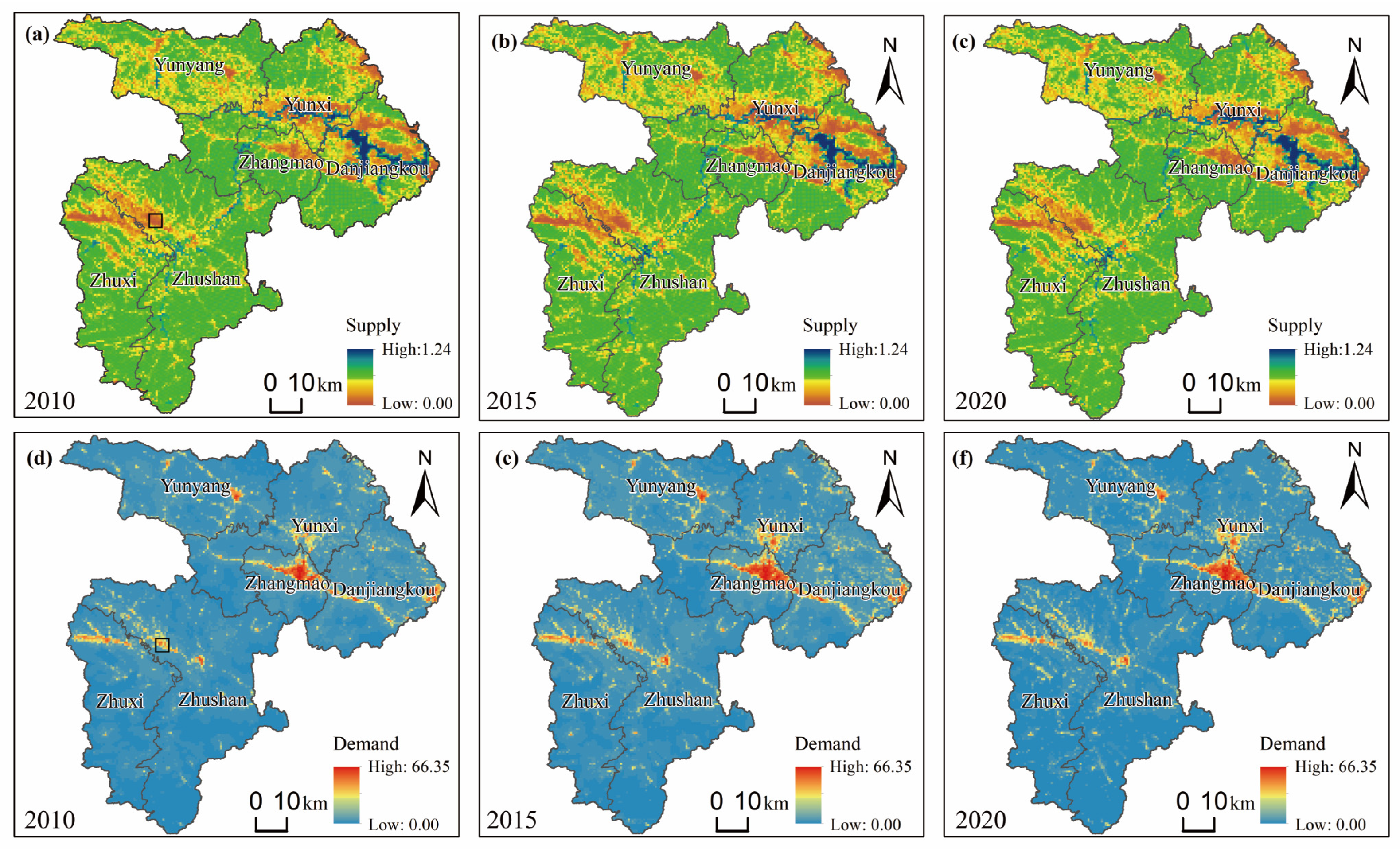
2.1. Study Area and Data

The content of ecosystem service (ES) supply and demand is extensive, with land use changes, demographic shifts, and economic conditions induced by urbanization standing out as the most prominent indicators. Urban land represents the intensity of human consumption of ecosystems, population density directly indicates the level of human demand on environmental systems, and economic density reflects economic development levels and indirectly reflects human preferences for natural systems [24,31]. Therefore, this study focuses on urban land proportion, population density, and economic density as research objects, and selects the Danjiangkou Basin (DB) in China for investigation and analysis. Located in northwest Hubei Province, China, as illustrated in Figure 1, the Danjiangkou Basin covers a total area of 21,000 square kilometers and comprises six cities. This region boasts advantageous natural conditions and a continually advancing urbanization process. Due to variations in urbanization levels and ecological conditions, the balance between ES supply and demand is increasingly tipping. It is impractical to halt or reverse urbanization to address this trend. Exploring urban spatial development patterns, particularly compact spatial development models, to develop land cautiously and effectively, minimize disruption to the urban landscape, mitigate this disparity, and achieve sustainable ecosystem service development, is a highly worthwhile endeavor.

To analyze the inequality in ecosystem service (ES) supply and demand across different levels of urbanization in the region, we divided the area into three subregions, based on urban land use: developed areas, developing areas, and rural areas, as illustrated in Figure S1. Developed areas are those classified as urban land in 2000, 2015, and 2020. Developing areas encompass lands designated as rural in 2000 and 2015, but reclassified as urban in 2015 and 2020, respectively. Rural areas are those identified as rural in 2000, 2015, and 2020.

For spatial statistics and analysis, we collected land use data with a 30 m resolution for the years 2010, 2015, and 2020 from the Resource and Environment Science Data Center (RESDC) of the Chinese Academy of Sciences (http://www.resdc.cn, accessed on 6 March 2024). The original data encompass six primary land use types (arable land, forestland, grassland, water bodies, construction land, and unused land), along with population density and GDP per unit of land for the region in 2010, 2015, and 2020. To ensure data compatibility, all data were spatialized into uniform grid cells, each covering an area of 1 km × 1 km.

2.2. Improved ES Supply–Demand Inequality Assessment

Accurately assessing supply–demand inequality in ecosystem services (ESs) is essential for effective management. To achieve this, we initially defined a grid-based ecosystem service (ES) supply and demand model, alongside a traditional Gini coefficient evaluation approach. Following this, we enhanced the traditional Gini coefficient by incorporating spatial proximity and clustering effects into the assessment of local inequality, thereby formulating a local Gini coefficient. This enhancement is aimed at mitigating the impact of spatial variations.

2.2.1. Grid ES Supply–Demand Model

Measuring the demand for ecosystem services (ESs) requires identifying key indicators that reflect urbanization dynamics. Based on the research findings of [31], this paper selects three key indicators—urban land proportion, population density, and economic density—to measure the demand for ecosystem services (ES). A model for ES demand within each grid is established as follows:

$$ESD{I}_i=D_i\times lo\mathrm{g}\left(P_i\right)\times lo\mathrm{g}\left(E_i\right),$$

(1)

where ${ESDI}_i$ is ES demand in the $i_{th}$ grid; and $D_i$, $P_i$, and $E_i$ represent the proportion of urban land, the population density (people/km²), and the economic density (10⁴ RMB/km²), respectively.

Building upon the table of equivalent factors for ecosystem service value per unit area in China established by Xie et al. [32], and the modification strategy based on forest cover for natural environments proposed by Xu et al. [33], this paper adopts the following formula for adjustment:

$$N={\displaystyle \frac{f_y}{F_y}},$$

(2)

where $N$ is the correction coefficient, $f_y$ is the average value of Fractional Vegetation Cover (FVC) in the DB region, and $F_y$ is the average value in China. $y$ refers to a specific year (i.e., 2010, 2015, and 2020).

Combining the grid-based ecosystem service (ES) demand model with the ecosystem service value assessment algorithm per unit area, the ES supply model adopted in this paper is as follows:

$${ESSI}_i=\sum _{j=1}^4{A}_j\times P_{ij}\times N,$$

(3)

where ${ESSI}_i$ is the function of ESs of category I_i in the region, $A_j$ is the area of land type $j$, and $P_{ij}$ is the type $i_{th}$ ES function unit area value of land type $j$ in China (Table S1).

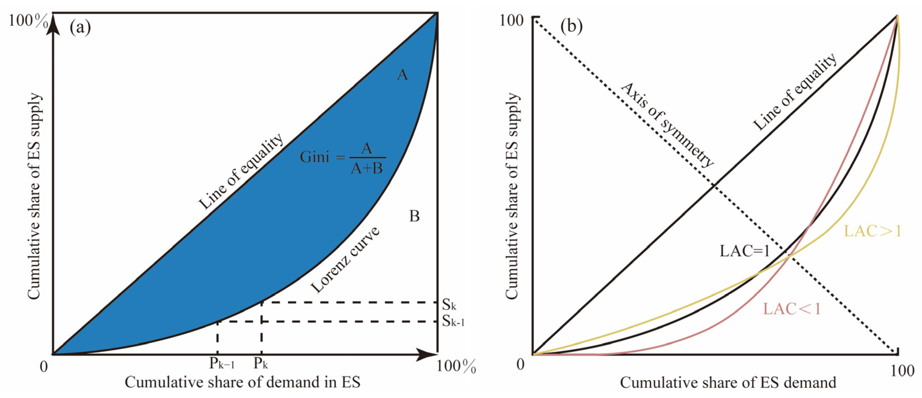
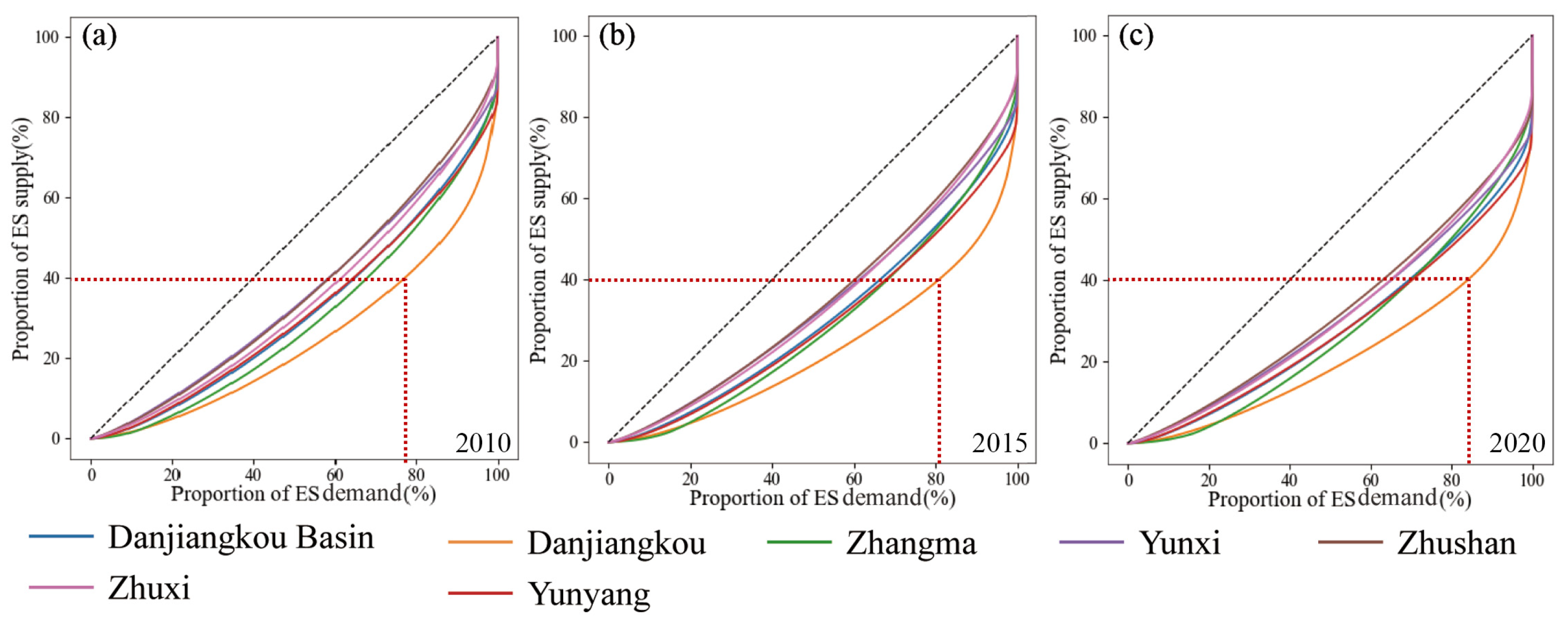
2.2.2. Gini Coefficient and Lorenz Asymmetry Coefficient

Assessing the degree of inequality in ecosystem service (ES) supply and demand requires reliable statistical tools. The Gini coefficient and the Lorenz Asymmetry Coefficient (LAC) are classic tools for this assessment. The principle of the Gini coefficient is illustrated in Figure 2a, with values ranging from 0 to 1, where higher values indicate greater inequality in the distribution of ES supply and demand. For this study, we present the specific expression for the Gini coefficient as follows:

$$G=1-2\sum _{k=1}^n\left(P_k-P_{k-1}\right)\left(S_k+S_{k-1}\right),$$

(4)

where $G$ is the Gini coefficient; $k$ is the index of the analysis unit, which is produced by sorting the analysis units; $n$ represents the number of analysis units; $P_k$ represents the cumulative proportion of ES demand; and $S_k$ represents the cumulative proportion of ES supply.

The Lorenz Asymmetry Coefficient (LAC) can elucidate which categories have the greatest impact on inequality. The evaluation principle is illustrated in Figure 2b. When a point lies above the axis of symmetry and the LAC is greater than 1, it indicates that inequality is primarily influenced by a minority of basic service demand entities that benefit from a large supply of these services. Conversely, when the point lies below the axis of symmetry, resulting in a LAC of less than 1, the inequality shifts accordingly [19].

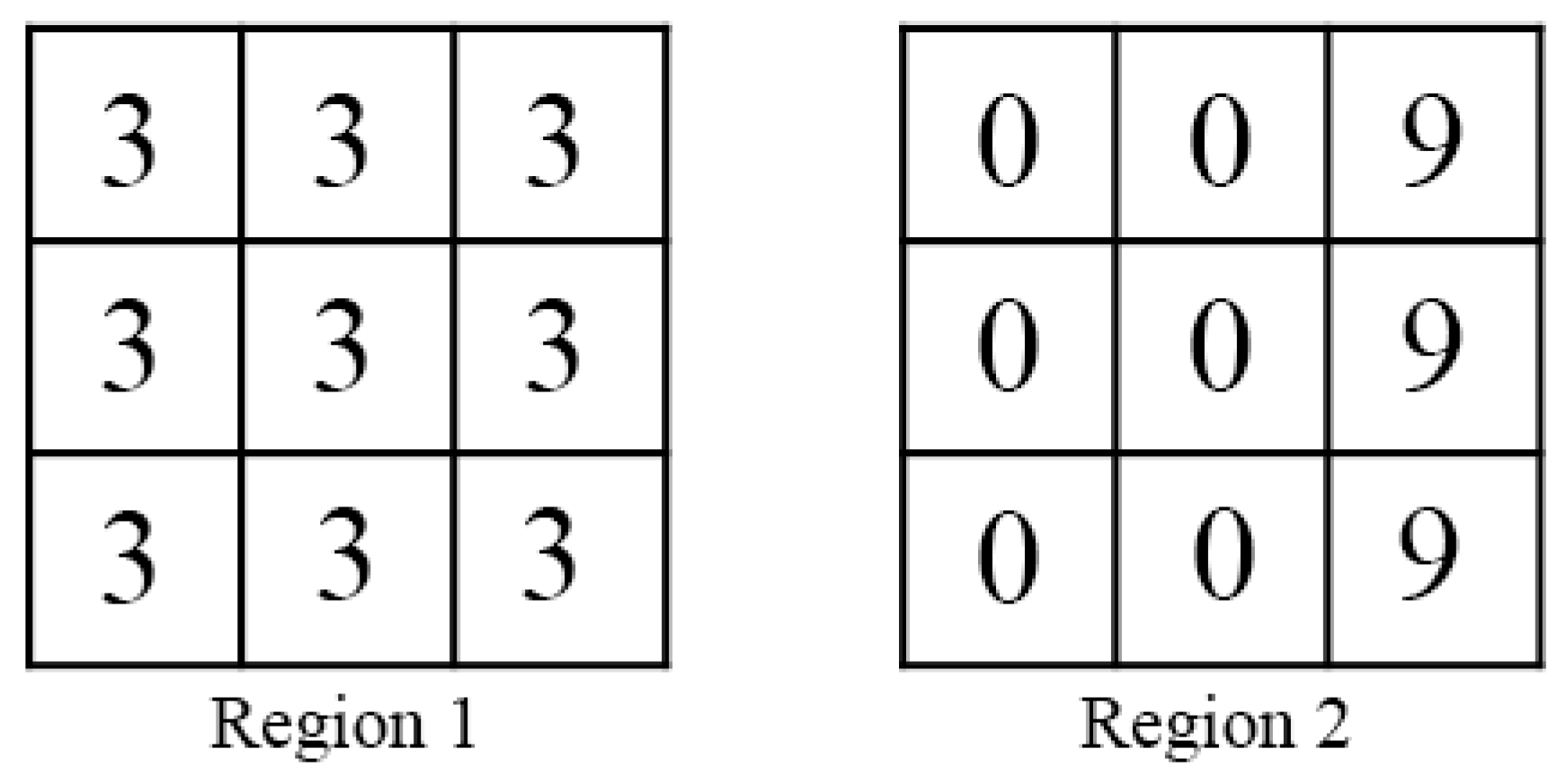
2.2.3. Local Gini Coefficient

Quantifying inequality in ecosystem service (ES) supply and demand within individual grids fails to capture inter-grid disparities. To address this, we propose a combined approach using the Gini coefficient and a moving window, as shown in Figure S2. This method emphasizes the spatial interaction between ES demand (supply) within a window centered on each pixel, and the surrounding ES supply (demand). We refer to this as the local Gini coefficient. The local Gini coefficient requires uniform processing within an $n$ × $n$ window ($n$ = 3) constructed from a 1 km × 1 km grid. Based on this setup, the distance from the center grid cell to the peripheral grid can be between 1 and 1.5 km, which approximates the walking distance for pedestrians within 15 min. This design is supported by the “Technical Guidelines for Community Living Circle Planning” published by the state in 2021; the guidelines specify that a 15 min community living circle should meet the various public service facility needs of residents within walking distance. Therefore, we employ a 3 × 3 moving window algorithm to more accurately and scientifically reflect the quantitative assessment of the inequality in supply and demand for ecosystem services centered on human needs. For each grid, the local Gini coefficient can be calculated using the following formula:

$$G_{ij}=1-2\sum _{k=1}^N\left(D_{ij,k}-D_{ij,k-1}\right)\left(S_{ij,k}+S_{ij,k-1}\right),$$

(5)

where $G_{ij}$ represents the Gini coefficient for the grid located at the $i_{th}$ row and $j_{th}$ column. $D_{ij,k}$ and $S_{ij,k}$ represent the cumulative proportion of ES demand and supply, respectively, within an $n$ × $n$ window at the $i_{th}$ row and $j_{th}$ column, where $N$ refers to the number of the grids ($N$ = 9).

2.3. Urban Compactness Index

Measuring urban compactness is essential for understanding its impact on ecosystem services (ESs). Drawing upon research by Henderson et al. [34], we formulated an “urban compactness index” (UCI) based on the coefficient of variation term, capturing the compactness effect through economic density and urban morphology. Urbanization encompasses three aspects: population, economy, and land use. To eliminate spatial structural biases among these three aspects, it is necessary to integrate them and create a composite index.

$${UCI}_{ij}=1+CV(P_{ij}{)}^2,$$

(6)

$$P_{ij}={\displaystyle \frac{{PD}_{ij}+{GD}_{ij}+{ULP}_{ij}}{3}},$$

(7)

where ${UCI}_{ij}$ represents the spatial compact index of the grid in the $i_{th}$ column and the $i_{th}$ row. A higher value of ${UCI}_{ij}$ indicates a more compact spatial structure, whereas a lower value indicates more dispersion. $P_{ij}$ represents the spatial comprehensive development intensity of the grid in $i_{th}$ column and th $i_{th}$ row, and $CV$ represents the coefficient of variation of $P_{ij}$ of the grid in the $i_{th}$ column and the $i_{th}$ row. Finally, we incorporate $P_{ij}$ into the moving window algorithm to calculate ${UCI}_{ij}$ for each grid.

Understanding the urban compactness index (UCI) requires a comparative analysis of different spatial patterns. To further explore this, we consider two distinct regions: Region 1 and Region 2, as shown in Figure 3. Region 1 exhibits a dispersed spatial pattern. In contrast, Region 2 demonstrates a compact spatial pattern. Both regions contain an equal total number of P (i.e., 27), urban areas (i.e., 9), and density of P (i.e., 3). In Region 1, spatial development is scattered, with a density of 3, while in region 2, development is concentrated on the right half, with a density of 9, and a density of 0 on the left half. By applying Equations (6) and (7), for Region 1, the coefficient of variation term is calculated as 1, and for Region 2, it is calculated as 2. This reveals that under the same conditions of region area and average intensity (), a more concentrated distribution of spatial patterns leads to an increase in the coefficient of variation term. Thus, the coefficient of variation term can effectively represent the spatial patterns of a region. Based on this calculation principle, we embed this formula within a 3 × 3 moving window, similar to the method used for calculating local inequality in ecosystem service (ES) supply and demand.

Furthermore, we calculated the population, economy, and urban land within each 1 km × 1 km grid as the urban average density, represented as urban land/km², RMB/km², and population/km², respectively.

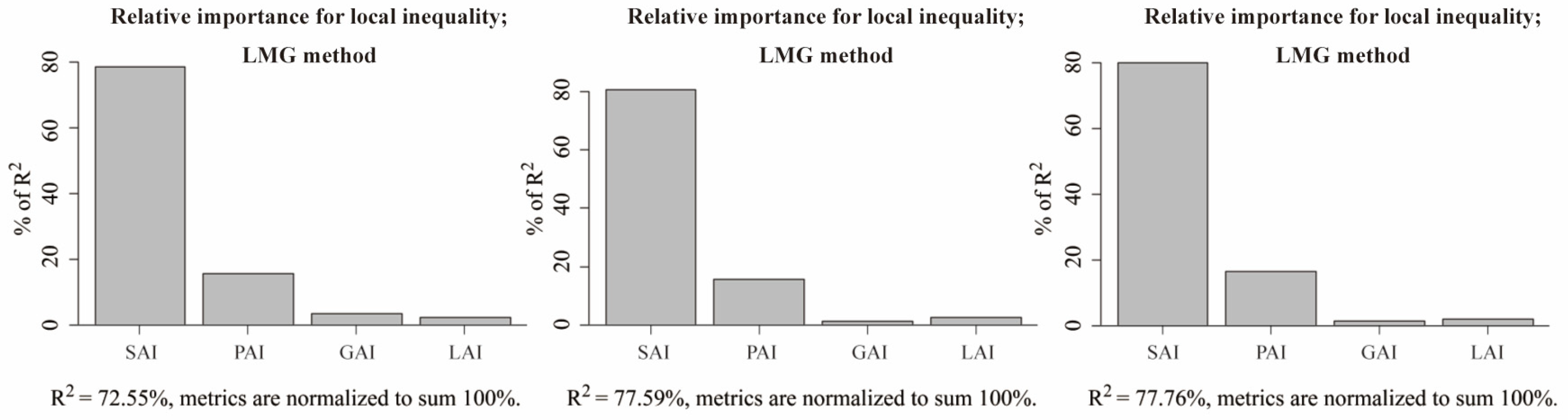
2.4. Statistical Analysis

Analyzing the relationship between local inequality and various influencing factors requires robust statistical methods. We employ the Ordinary Least Squares (OLS) regression technique. OLS calculates the regression coefficients by minimizing the sum of squared errors between the theoretical values predicted by the model and the observed values [35]. OLS can be succinctly represented as follows:

$$Y={\beta }_0+{\beta }_1{X}_1+{\beta }_2{X}_2+\dots +{\beta }_n{X}_n+\epsilon ,$$

(8)

where $Y$ is the dependent variable; ${\beta }_0$ is the constant; $x_n$ is the independent variable; ${\beta }_n$ is the partial regression coefficient; and $\epsilon$ is the residual.

Furthermore, to capture the spatial influence among variables at the local level, this paper adopts the Geographically Weighted Regression (GWR) method. Guided by Tobler’s First Law of Geography, GWR can reflect the relationships between neighboring entities [36,37]. The GWR equation can be represented as follows:

$$Y_i={\beta }_0\left(u_i,v_i\right)+{\beta }_1\left(u_i,v_i\right)X_{1i}+{\beta }_2\left(u_i,v_i\right)X_{2i}+\cdots +{\beta }_k\left(u_i,v_i\right)X_{ki}+{\epsilon }_i,$$

(9)

where $Y_i$ and $X_{ij}$ are the dependent and independent variables, respectively; $\left(u_i,v_i\right)$ are the coordinates of location $i$; ${\beta }_0\left(u_i,v_i\right)$ is the intercept; ${\beta }_j\left(u_i,v_i\right)$ (j = 1,…, k) is the coefficient at location $i$; and ${\epsilon }_i$ is the random error term.

3. Results

3.1. Global Inequality Estimates

The spatial distribution of ecosystem service (ES) supply–demand displays contrasting trends along the urban–rural gradients, with high demand and weak supply in urban areas, and the opposite in suburban and rural areas (Figure 4). ES supply showed the highest value in the northeast of the study area, mainly in the Danjiangkou Reservoir area where large expanses of water bodies occurred. However, the majority of ES supply was located in non-built-up areas of Zhushan, Danjiangkou, and Yunyang, collectively contributing more than 60% to the total ES supply (Table S2). Moreover, the ES supply maintained relative stability, not only in its spatial distribution, but also in quantity, with values of 47.17 million in 2010, 47.54 million in 2015, and 47.77 million in 2020. In terms of ES demand, the most critical areas for ES demand were concentrated in the main urban areas of various counties, especially in Zhangmao, which accounted for 50% of the total ES demand (Table S2). Generally, there was a gradual decline in the intensity of ES demand from the city center to the suburbs. Unlike the ES supply, the ES demand range showed a trend of continuous spatial expansion, due to urban expansion. Correspondingly, the values of ES demand increased from 6157 in 2010 to 12,320 in 2020, highlighting the growing pressures on urban resource management.

The global inequality varied among cities and increased over time within the same city (

Table 1. Evaluation of the Gini coefficient for ecosystem service supply–demand in different cities.

City Year	DB	Danjiangkou	Zhangmao	Yunyang	Yunxi	Zhushan	Zhuxi
2010	0.370	0.512	0.413	0.369	0.290	0.283	0.320
2015	0.393	0.545	0.419	0.415	0.329	0.307	0.326
2020	0.432	0.572	0.450	0.441	0.379	0.350	0.370
Average	0.398	0.543	0.427	0.408	0.333	0.313	0.339

). The highest average Gini coefficient was 0.543 in Danjiangkou, while the lowest was 0.313 in Zhushan. Furthermore, the global inequality of ES supply–demand in each city gradually increased over time, related to the faster growth of ES demand compared to ES supply. We also calculated the LAC for each city to further analyze the disparities in global inequality among cities. We found that the LAC of most cities was greater than 1, indicating that inequality is driven by limited ES demand being met with abundant ES supply, while only Yunyang had a LAC of less than 1. Additionally, an intriguing observation is that despite sharing the same Gini coefficient, Zhangmao and Yunyang exhibited widely differing LACs. This effectively demonstrates that, even with identical Gini coefficients, the spatial matching patterns of ES supply–demand can vary significantly. Furthermore, the Lorenz curve offers insights into the spatial distribution disparities between supply and demand (Figure 4). For example, global inequality in Danjiangkou increased from 0.370 in 2010 to 0.432 in 2020 (Table 1), and this worsening trend is also evident in the corresponding Lorenz curve, where an equal amount of ES supply (40%) is shared among continuously increasing ES demand (78–83%) in 2010, 2015, and 2020 (Figure 5). This analysis highlights the complex dynamics of ES supply–demand inequality and its implications for resource management.

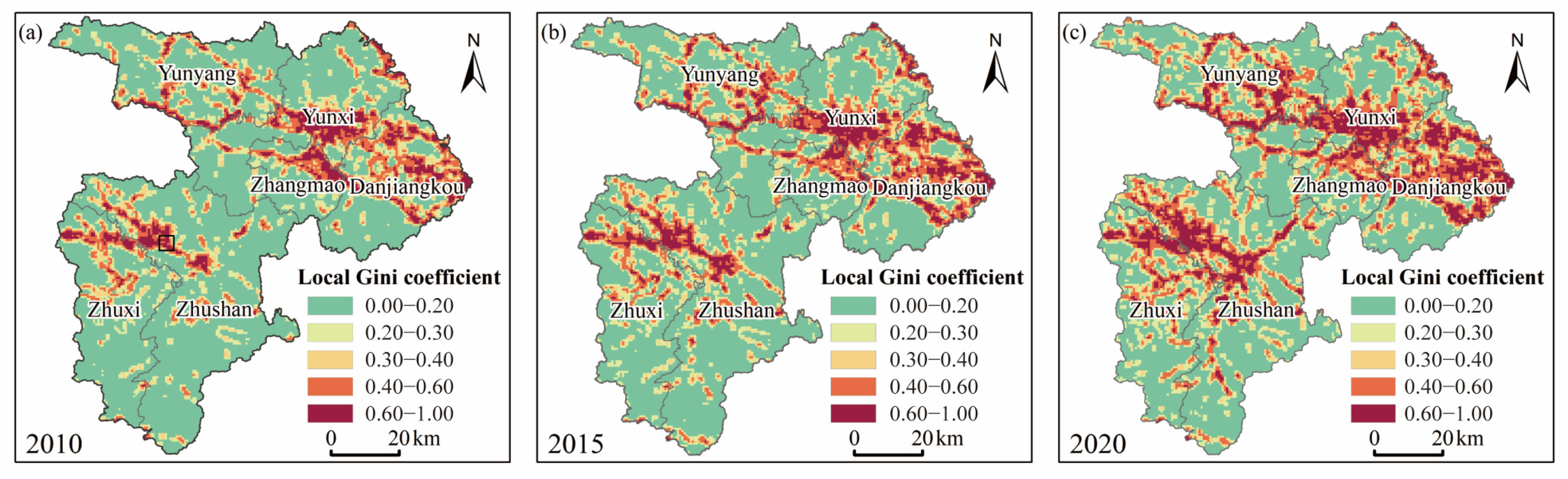
3.2. Local Inequality Estimates

The spatial distribution of local inequality in ecosystem service (ES) supply–demand showed a distinct center–fringe structure (Figure 6). Higher local inequality (0.6–1.0) was predominantly observed in highly urbanized areas, where large populations, economies, and urban land uses are concentrated. Lower local inequality (0.0–0.2) was mainly distributed in remote urban areas, characterized by abundant forests and grasslands. Intermediate levels of local inequality (0.2–0.6) were found along transportation networks and at urban–suburban interfaces. Over time, the scope of local inequality expanded outward along urban boundaries, particularly in areas where urban expansion was high. Additionally, the transportation networks connecting different cities emerged as key foci of local inequality evolution from 2010 to 2020, with the pattern of change shifting from points to lines.

The trend of localized inequality in ecosystem service (ES) supply–demand varied significantly across regions with different levels of urbanization (

Table 2. The proportion and local inequality in different development regions.

Year	Rural Areas		Developing Areas		Developed Areas
	Proportion	Local Gini Coefficient	Proportion	Local Gini Coefficient	Proportion	Local Gini Coefficient
2010	74.66%	0.108	19.04%	0.307	6.30%	0.518
2015	68.24%	0.108	23.18%	0.313	8.57%	0.543
2020	58.67%	0.110	28.89%	0.316	12.44%	0.558
Average	67.19%	0.109	23.70%	0.312	9.10%	0.54
2010–2020	−15.99%	0.002	9.85%	0.009	6.14%	0.04

). Developed regions experienced a substantial rise in local inequality, increasing by 0.04, from 0.518 in 2010 to 0.558 in 2020. Secondly, developing areas exhibited a slower increase of 0.009, from 0.307 in 2010 to 0.316 in 2020. Meanwhile, local inequality in rural areas remained relatively stable. Additionally, regarding changes in the scope of localized inequality, an opposite pattern was observed. Rural areas experienced the most significant decrease, by 15.99%, due to urban expansion. Conversely, developing regions saw the largest increase, by 9.85%, while developed regions saw an increase of 6.14%.

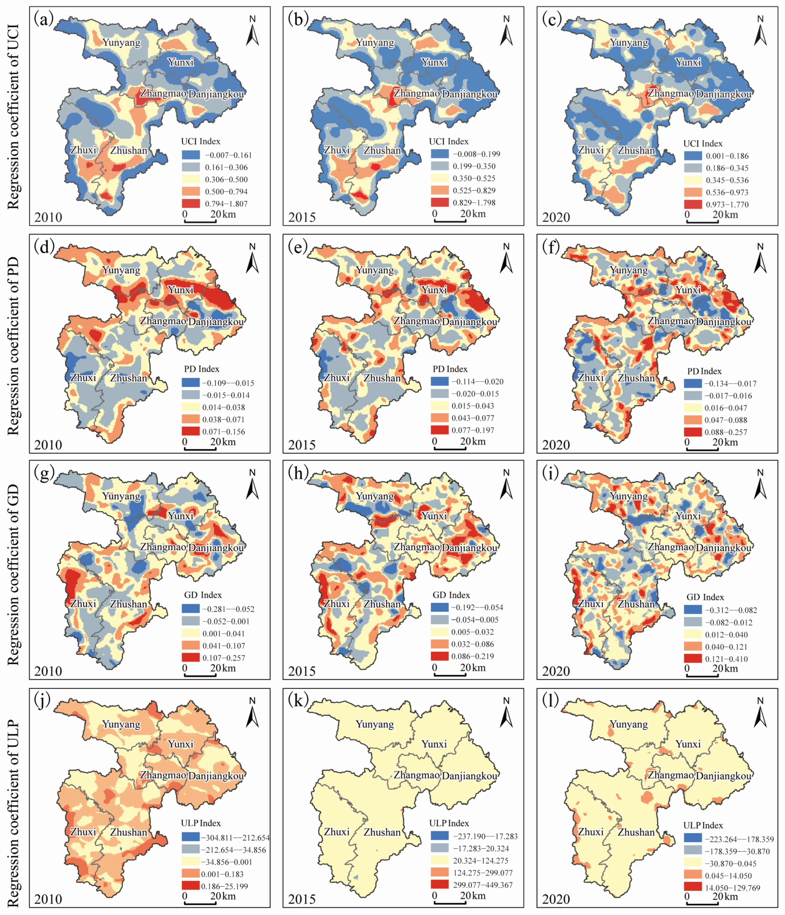
3.3. Global and Local Regression Results

Assessing the impact of urbanization on local inequality is essential for effective urbanization processes. To evaluate this impact, we employed an OLS model to evaluate two dimensions: urban development intensity and spatial compactness. The OLS model accounted for over 60% of the variation in local inequality over time (

Table 3. Parameters and Statistics for the spatial Gini coefficient with Ordinary Least Squares regression and Geographically Weighted Regression models.

		OLS		GWR
		Coef.	S.E.	Min.	First Qu.	Median.	Third Qu.	Max.
2010	Intercept	−0.259 ***	0.0028	−50.321	−0.493	−0.350	−0.171	602.408
	UCI	0.150 ***	0.0015	−0.007	0.142	0.215	0.375	1.807
	ULP	0.022 **	0.0135	−304.811	−0.002	0.008	0.021	25.200
	P D	0.032 **	0.0004	−0.110	0.006	0.023	0.044	0.156
	GD	0.023 *	0.0006	−0.282	−0.009	0.011	0.037	0.257
	AICc	48,072.430		45,741.581
	Adjusted R-squared	0.607		0.828
2015	Intercept	−0.245 ***	0.0028	−890.977	−0.558	−0.377	−0.176	468.447
	UCI	0.160 ***	0.0015	0.008	0.151	0.240	0.386	1.799
	ULP	0.023 **	0.0135	−237.191	−0.002	0.007	0.020	449.367
	PD	0.034 **	0.0004	−0.115	0.006	0.025	0.045	0.197
	GD	0.014 *	0.0006	−0.193	−0.007	0.012	0.040	0.219
	AICc	50,882.60		48,795.406
	Adjusted R-squared	0.653		0.855
2020	Intercept	−0.223 ***	0.0037	−258.115	−0.559	−0.317	−0.014	440.848
	UCI	0.140 ***	0.0013	0.000	0.125	0.226	0.382	1.770
	ULP	0.021 **	0.0106	−223.265	−0.002	0.007	0.019	129.769
	PD	0.039 **	0.0005	−0.135	0.003	0.025	0.053	0.258
	GD	0.015 *	0.0006	−0.312	−0.022	0.008	0.040	0.411
	AICc	49,736.50		45,902.796
	Adjusted R-squared	0.648		0.879

Note: ***, **, and * represent 1%, 5%, and 10% significance levels, respectively.

). The results suggest that all metrics had a positive influence on local inequality, with the urban compactness index (UCI) demonstrating the highest relative importance, explaining 79% of the model’s variance (Figure 7). Population density (PD) emerged as the second most influential predictor, contributing 16% to the model’s explanatory power (Figure 7). These findings underscore the significance of integrating multi-dimensional urbanization elements into modeling frameworks, for more accurate estimation of local inequality compared to single urbanization metrics. In contrast, GDP density (GD) and urban land proportion (ULP) had a lower relative importance, each contributing only 5% to local inequality in ES supply–demand.

The assumption of a stationary relationship in the OLS model limits its ability to capture spatial heterogeneity in local inequality. To address this limitation, we employed the GWR model to comprehensively assess the impacts of urbanization density and spatial compactness on local inequality. The diagnostic information presented in Table 3 reveals that the GWR model outperformed the OLS model, demonstrated by lower Corrected Akaike Information Criterion (AICc) values and higher adjusted R-squared values [38]. The adjusted R-squared value notably increased from 0.607 in the OLS model to 0.879 in the GWR model, indicating that the local regression model could account for over 80% of the variation in local inequality. Additionally, the significant decrease in AICc values for the GWR model compared to the OLS model indicates comparatively excellent retention of crucial information.

The relationship between urbanization indicators and local inequality is complex and varies spatially. The spatial distribution of GWR coefficients (Figure 8) indicates that all four indicators in the two dimensions positively impact local inequality, although their influence changes direction along the urban–rural gradient. The regression coefficients for the UCI indicator steadily increase from the city center to the urban periphery, potentially influenced by the predominant land use types in these areas. In city centers, characterized by predominately residential and commercial land use, the concentrated residential patches have a minimal impact on local inequality. Conversely, non-urban areas dominated by rural settlements feature a dispersed spatial structure with ample development space, facilitating aggregation and potentially elevating local inequality. Regarding urbanization indicators, the impact of population density and GDP density on local inequality lessens from urban centers to suburbs. Higher regression coefficients in central urban areas suggest that increased population or GDP densities may correspond to greater local inequality. Conversely, smaller regression coefficients in some remote areas indicate that the impact of urbanization development on local inequality is relatively weak.

4. Discussion

4.1. Impact of ES Supply–Demand Inequality on Ecological Management System

Ecosystem service (ES) supply–demand inequality exhibits spatial scale effects. Thus, ecological management must accurately portray supply–demand relationships across multiple scales. Boithias et al. [39] and Yin et al. [40] have observed that notable supply–demand inequalities at the local scale can be alleviated at the global scale. However, we argue that such mitigation predominantly arises from averaging effects, which fail to account for local-scale disparities. Therefore, capturing overarching trends at the global scale is crucial. It is equally imperative to conduct thorough assessments and analyses at the local scale. Integrating these evaluation results into corresponding ecological decision-making processes provides a foundational basis for regional resource management and allocation.

The progressive intensification of global ecosystem service (ES) supply–demand inequality from 2010 to 2020 highlights the need for targeted strategies to address the imbalance between supply and demand. This trend is evident not only in the DB region, but is also likely prevalent at other regional and national scales [2,41,42]. While this escalating inequality has been attributed to both a surge in demand and a decline in supply [26], our study reveals a nuanced finding: both ES supply and demand increased during this period, but the growth in demand outpaced the growth in supply. Specifically, in the DB region, ES demand surged by 6163 units, whereas ES supply increased by 0.6 million units from 2010 to 2020.

Although global-scale ecosystem service (ES) inequality provides a macro-perspective for understanding, local-scale inequality can better capture the spatial details of ES inequality. In this study, local inequality showed a diminishing trend with increasing distance from the city center. Over time, the range of local inequalities gradually expanded. This ring structure aligns with findings from other researchers in regions such as Madrid, Spain, in the work of Baró et al. [43], Berlin, Germany [44], and Tianjin, China, in the work of Li et al. [45], all of which display a center–periphery structure. However, this structure does not adequately reflect the impact of spatial proximity and clustering on local inequality. To address this limitation, our study introduces a moving window Gini coefficient algorithm. This algorithm captures the mismatch between natural resources and social demands within a single grid. It also accounts for inequalities arising from disparities in ES supply–demand among neighboring grids. The moving window Gini coefficient algorithm is characterized by strong continuity, and incorporates spatial QUEEN proximity weights. It effectively expresses the supply–demand relationship between a grid and its neighboring units, as well as accounting for the likelihood of residents obtaining ESs from surrounding grids. The advantages of the moving window algorithm over traditional supply–demand ratio algorithms are illustrated in Figure 9. Traditional algorithms treat individual grids as independent units, and insufficiently consider the mutual influence of adjacent grids. Consequently, differences along the boundaries of neighboring grid units are exaggerated, and edge effects significantly impact measurement accuracy. This makes traditional algorithms inadequate for indicating residents’ access to surrounding ESs. From an extreme perspective, if a central grid has only ES demand but no supply, while surrounding grids have high ES supply, the grid-based supply–demand ratio algorithm would classify this grid as experiencing a severe ecological deficit. In contrast, the moving window Gini coefficient algorithm would assess this grid as having relatively low ES supply–demand inequality, emphasizing the importance of a nuanced approach to understanding local disparities.

Another crucial aspect of incorporating ecosystem service (ES) supply–demand inequality into ecological management systems involves linking ecological issues across different scales with hierarchical decision-making frameworks. This linkage fosters horizontally integrated and vertically coordinated policy management, as well as ecological restoration measures. In this study, global inequality reveals disparities in ES supply–demand among counties. The accompanying LAC analysis of the Gini coefficient helps to identify the underlying causes of these disparities. When the LAC is greater than 1, inequality is primarily driven by a small number of ES demands receiving a large share of supply. Conversely, when the LAC is less than 1, inequality arises mainly from numerous ES demands matching a limited supply. For instance, despite similar levels of global ES supply–demand inequality between Zhangmao and Danjiangkou, the former is driven by excess demand exceeding supply, whereas the latter is characterized by oversupply relative to demand. Consequently, importing ES from Danjiangkou to Zhangmao could alleviate this supply–demand inequality. However, most ecological management decisions are implemented at the local scale. Therefore, local-scale assessments are essential for accurately determining the location, intensity, and extent of ES supply–demand gaps. They are also crucial for promoting precise intervention measures. For example, as nearby ecological resources supporting urban areas diminish, ES supplies need not be imported from farther locations. By comparing the degrees of local inequality, we can identify ecosystem providers, sinks, and the flow corridors necessary for transmitting ecosystem benefits to humanity.

In summary, the analysis of global inequality and LACs offers profound insights into the cross-county outflow or inflow of ecosystem services (ESs). This understanding facilitates the seamless integration of the ES framework into city-level ecological management and planning systems. By quantifying ES supply–demand inequality at the local scale, decision-makers can implement planning interventions and policies with heightened precision and localization, thereby minimizing the loss of critical ecosystems. Consequently, quantifying inequality across scales, from the global to the local scale, enables a more holistic accommodation of the needs of multi-level planning and management. In this framework, upper-level scales exercise control and regulation over lower-level scales. Meanwhile, lower-level scales contribute to the incremental refinement and implementation of upper-level planning objectives.

4.2. Driving Factors and Spatial Heterogeneity of ES Supply–Demand Inequality

The inequality of ecosystem service (ES) supply–demand results from the interaction between population growth, economic activities, and urban expansion at specific locations. To clarify the relationship between ES supply–demand inequality and the urbanization process, this study initially conducted a global regression analysis utilizing the OLS model. The results indicate that all indicators have a positive impact on local inequality. The urbanization process inevitably results in the encroachment of ecological land (including compact urban development), which is accompanied by an augmentation in ES demand, ultimately intensifying the disparity in ES supply–demand; these findings align with previous research conducted by Maimaiti, Chen, Kasimu, Simayi, and Aierken [10], and Gao et al. [46]. Furthermore, our analysis reveals that, compared to urbanization indicators, the urban compactness index (UCI) possesses the strongest explanatory power for ES supply–demand inequality, accounting for 79% of the model’s explanatory capacity. This may be attributed to the fact that urban compactness encompasses multiple dimensions, including population density, economic density, and land use, unlike individual factors. Additionally, the coefficient of variation term accounts for spatial compactness in areas with identical average densities but differing spatial distribution patterns. The interaction between these factors significantly enhances the explanatory power regarding ES supply–demand inequality, and underscores the importance of considering multiple dimensions in future analyses.

Although OLS identified several factors influencing supply–demand inequality, it is a non-spatial regression. In this model, the regression parameters are independent of the geographical locations of the sample data [27]. To address this limitation, we conducted further analysis using the GWR technique. This approach accounts for spatial heterogeneity and provides a clearer observation of spatial relationships and trends among variables [36,47,48]. These characteristics are essential for determining where and how to manipulate various urbanization drivers in order to effectively rebalance sustainable ES supply–demand. In this study, the magnitudes and directions of the GWR coefficients for the urban compactness index and urbanization indicators exhibited contrasting spatial trends. Specifically, the GWR coefficient for spatial compactness showed a gradually increasing trend (from small to large) from urban centers to suburbs and rural areas. This transition indicates that in urban centers, the increase in spatial compactness has a negative or weaker correlation with ES supply–demand inequality. Conversely, in non-urban areas with smaller populations and sparser artificial land use, the GWR coefficients for compactness were larger. This suggests that the introduction of high-density compact development in these areas can readily disrupt the existing supply–demand balance. However, the GWR coefficients for urbanization indicators showed a gradually decreasing trend from urban centers to suburbs and rural areas. This reflects that an increase in population, economy, and urban land use in urban centers can exacerbate ES supply–demand inequality, while this effect is weaker in suburbs and rural areas. Overall, suburban and rural areas typically maintain better ecological resources, and small-scale urbanization processes are less likely to disrupt the original ES supply–demand balance.

4.3. Regional Ecological Governance Should Adopt a Spatially Based Hierarchical Layout

The disparities in ecosystem service (ES) supply–demand inequality across various scales offer targeted insights for ecological governance at diverse levels. This enables the equitable development of ES supply–demand through cross-scale sharing of essential components. In this study, a global-scale analysis identified disparities in global inequality. It also elucidated whether these disparities are primarily driven by excess supply compared to demand, or vice versa, thereby fostering cross-regional flows of ES. Additionally, assessments conducted at the local scale can precisely identify the intensity, location, and scope of ES supply–demand disparities. These assessments serve as the foundation for implementing locally tailored ecological governance measures. Consequently, the development of multi-scale ecological governance strategies is crucial. These strategies should be supported at upper scales, and refined and optimized at lower scales. This represents a pivotal pathway toward achieving equitable development in ES supply and demand.

Assessing ecosystem service (ES) supply–demand inequality at the global scale plays a crucial role in the formulation and implementation of macro-level policies. At the regional level, the alignment between ES supply–demand within the DB area is generally satisfactory. However, disparities in supply–demand inequality persist among different counties. Given this situation, it is imperative to evaluate the intricate dynamics of ES supply–demand from a broader perspective. This perspective should encompass the interactions between cities and their adjacent environments. A holistic view will inform strategies for importing or exporting ESs from or to other regions. By fostering county-level coordination, we can enhance inter-regional collaborative ecosystem management and realize mutual benefits. In this study, we employed the Gini coefficient to quantify ES supply–demand inequality among counties. For counties exhibiting substantial variations in the Gini coefficient, we further compared their corresponding LACs. If the LAC is greater than 1, it indicates that the county serves as a potential outflow area with abundant ES supply. Conversely, an LAC less than 1 suggests that the county requires ES inputs to satisfy excess demand. In the experimental area of this study, Zhangmao County accounted for 55% of the total ES demand, but contributed only 6% to the total supply (Table S2), with an LAC below 1. Therefore, ecological resources can be strategically transferred from neighboring counties to Zhangmao County.

Evaluating ecosystem service (ES) supply–demand inequality at the local scale can guide the implementation of differentiated administrative decisions. The local scale can be seen as a continuation of the global scale structure. It accommodates the flow of ESs across counties, and enables their distribution and refinement within local spaces. In this study, we propose reallocating ESs flowing into the main urban area of Zhangmao from other counties. Specifically, we propose the alleviation of supply–demand contradictions by augmenting ecological landscapes within the urban core, such as establishing at least one substantial ecological space (e.g., pocket parks, green squares) in various neighborhoods [2,48,49]. Additionally, our research uncovers significant inequality in ES supply–demand along the roads connecting counties. Consequently, enhancing the construction of ecological corridors along these roads and improving ES accessibility can facilitate the remote coupling of ES supply–demand [9,50]. In terms of urban development, the estimation coefficients derived from this study provide valuable insights for local and regional entities, such as counties. These insights will help them to better comprehend the ramifications of their planning and development strategies on future ES demand. Notably, compared to suburbs and rural areas, the estimation coefficient for compactness indices in urban core areas is smaller. In contrast, the estimation coefficient for urbanization indicators is larger. This indicates that urbanization tends to exacerbate local inequality, while spatially compact development mitigates this inequality. Therefore, adopting compact spatial development strategies within large-scale urbanization projects can serve as an effective means to alleviate local inequality.

4.4. Contributions and Limitations

This study presents significant improvements in the quantification methods and governance strategies for ecosystem service (ES) supply–demand inequality, with the following research significance. Methodological Innovation: By introducing a local Gini coefficient that incorporates a moving window, this study integrates spatial proximity and clustering effects into local inequality assessments. This approach overcomes the limitations of traditional Gini coefficients that neglect spatial heterogeneity, thus enhancing quantification accuracy. Theoretical Expansion: We constructed a multi-dimensional urban compactness index (UCI) that combines population, economy, and land use. This index highlights the crucial role of compact urban layouts in alleviating ES supply–demand conflicts, addressing the limitations of single indicators like population density. Practical Value: A hierarchical governance framework is proposed based on multi-scale analysis, offering a scientific basis for cross-county ecological coordination and sustainable urban development in the Danjiangkou Basin. This framework provides an actionable pathway for balancing ecological protection and resource management through compact development in highly urbanized areas. This research advances the theoretical development of methods for quantifying ES supply–demand relationships, and serves as an important reference for ecological governance and urban planning in similar global regions.

However, this study also has several limitations. Firstly, due to data constraints, our measurement of ES supply–demand primarily relied on land use data and socio-economic factors. We did not delve into specific ecological functions such as water provision, carbon sequestration, food production, and landscape esthetics. However, we adopted a holistic approach to representing ES supply–demand, and the absence of some data did not result in significant deviations in the conclusions. Secondly, while this study identified a gradient decline in ES supply–demand inequality along the urban–rural continuum, the spatial pattern of this gradient remains unexplored. This should be a focal area for future research endeavors. Lastly, our analysis centered solely on urbanization as a pivotal driving factor influencing ES supply–demand inequality. We overlooked other potential factors, such as the natural environment (including rainfall, temperature, terrain, and slope). This gap necessitates further exploration in subsequent studies.

5. Conclusions

This study took the Danjiangkou Basin (DB) in China as the research subject and established a global-to-local ecosystem service (ES) analysis framework to identify the spatial patterns of ES supply, demand, and inequality from a cross-scale perspective. It provides governance guidance for hierarchical ecological planning and management. The main conclusions are as follows:

Regarding the assessment of supply–demand inequality, we found that from 2010 to 2020, the global inequality in the study area gradually increased, rooted in the faster growth of ES demand compared to ES supply. This conclusion benefits from the adoption of the moving window Gini coefficient to quantify ES supply–demand inequality and LAC (Lorenz Asymmetry Coefficient) analysis, accurately identifying the quantity of ESs flowing into or out of counties across the region.

In terms of driving forces, we discovered that urbanization in the study area exacerbated ES supply–demand inequality. However, compact urban development could mitigate the intensification of inequality. This conclusion is based on our construction of an urban compactness index (UCI) using the coefficient of variation terms, which integrates multiple dimensions, such as population, economy, and urban land use, into a unified expression. Additionally, it incorporates spatial distribution patterns into the calculation of spatial compactness, thus enabling the index to possess comprehensive explanatory capabilities.

Regarding hierarchical governance, we believe that addressing the imbalance between ES supply and demand requires joint efforts at both the global and local levels. At the global level, this involves coordinating ES supply–demand complementarity among multiple regions, while at the local level, specific strategies, such as compact cities, can be adopted to restore ecology.

References

1. Costanza, R.; de Groot, R.; Braat, L.; Kubiszewski, I.; Fioramonti, L.; Sutton, P.; Farber, S.; Grasso, M. Twenty years of ecosystem services: How far have we come and how far do we still need to go? Ecosyst. Serv. 2017, 28, 1–16. [Google Scholar] [CrossRef]
2. González-García, A.; Palomo, I.; González, J.A.; López, C.A.; Montes, C. Quantifying spatial supply-demand mismatches in ecosystem services provides insights for land-use planning. Land Use Policy 2020, 94, 104493. [Google Scholar] [CrossRef]
3. Hou, Y.; Müller, F.; Li, B.; Kroll, F. Urban-Rural Gradients of Ecosystem Services and the Linkages with Socioeconomics. Off. J. Int. Assoc. Landsc. Ecol. (IALE-D), Landsc. Online 2015, 39, 1–31. [Google Scholar] [CrossRef]
4. Reid, W.; Mooney, H.; Cropper, A.; Capistrano, D.; Carpenter, S.; Chopra, K. Millennium Ecosystem Assessment: Ecosystems and Human Well-Being: Synthesis; Island Press: Washington, DC, USA, 2005. [Google Scholar]
5. Kundu, D.; Pandey, A. World Urbanisation: Trends and Patterns. In Developing National Urban Policies; Springer: Singapore, 2020; pp. 13–49. [Google Scholar]
6. Giannetti, B.F.; Agostinho, F.; Almeida, C.M.V.B. Chapter 2—Sustainable development and its goals. In Assessing Progress Towards Sustainability; Teodosiu, C., Fiore, S., Hospido, A., Eds.; Elsevier: Amsterdam, The Netherlands, 2022; pp. 13–33. [Google Scholar]
7. He, G.; Zhang, L.; Wei, X.; Jin, G. Scale effects on the supply–demand mismatches of ecosystem services in Hubei Province, China. Ecol. Indic. 2023, 153, 110461. [Google Scholar] [CrossRef]
8. Xia, H.; Yuan, S.; Prishchepov, A.V. Spatial-temporal heterogeneity of ecosystem service interactions and their social-ecological drivers: Implications for spatial planning and management. Resour. Conserv. Recycl. 2023, 189, 106767. [Google Scholar] [CrossRef]
9. Su, R.; Duan, C.; Chen, B. The shift in the spatiotemporal relationship between supply and demand of ecosystem services and its drivers in China. J. Environ. Manag. 2024, 365, 121698. [Google Scholar] [CrossRef]
10. Maimaiti, B.; Chen, S.; Kasimu, A.; Simayi, Z.; Aierken, N. Urban spatial expansion and its impacts on ecosystem service value of typical oasis cities around Tarim Basin, northwest China. Int. J. Appl. Earth Obs. Geoinf. 2021, 104, 102554. [Google Scholar] [CrossRef]
11. Qu, H.; You, C.; Wang, W.; Guo, L. Spatio-temporal interplay between ecosystem services and urbanization in the Yangtze River Economic Belt: A new perspective for considering the scarcity effect. Land Use Policy 2024, 147, 107358. [Google Scholar] [CrossRef]
12. Sylla, M.; Hagemann, N.; Szewrański, S. Mapping trade-offs and synergies among peri-urban ecosystem services to address spatial policy. Environ. Sci. Policy 2020, 112, 79–90. [Google Scholar] [CrossRef]
13. Zhou, L.; Zhang, H.; Bi, G.; Su, K.; Wang, L.; Chen, H.; Yang, Q. Multiscale perspective research on the evolution characteristics of the ecosystem services supply-demand relationship in the chongqing section of the three gorges reservoir area. Ecol. Indic. 2022, 142, 109227. [Google Scholar] [CrossRef]
14. Zhu, D.F.; Cao, H.; Luo, G.Y.; Pan, H.; Luo, C.Y. Simplified calculation and design method of multi-well system for anti-uplifting based on intercepting and discharging water. Yantu Gongcheng Xuebao/Chin. J. Geotech. Eng. 2021, 43, 1986–1993. [Google Scholar] [CrossRef]
15. Raudsepp-Hearne, C.; Peterson, G.D. Scale and ecosystem services: How do observation, management, and analysis shift with scale—Lessons from Québec. Ecol. Soc. 2016, 21, 16. [Google Scholar] [CrossRef]
16. Liu, M.; Xiong, Y.; Zhang, A. Multi-scale telecoupling effects of land use change on ecosystem services in urban agglomerations —A case study in the middle reaches of Yangtze River urban agglomerations. J. Clean. Prod. 2023, 415, 137878. [Google Scholar] [CrossRef]
17. Yi, D.; Guo, J.; Pueppke, S.G.; Han, Y.; Ding, G.; Ou, M.; Koomen, E. What dominates the variation of ecosystem services across different urban expansion patterns?—Evidence from the Yangtze River Delta region, China. Environ. Impact Assess. Rev. 2025, 110, 107674. [Google Scholar] [CrossRef]
18. Chen, Y.; Ge, Y.; Yang, G.; Wu, Z.; Du, Y.; Mao, F.; Liu, S.; Xu, R.; Qu, Z.; Xu, B.; et al. Inequalities of urban green space area and ecosystem services along urban center-edge gradients. Landsc. Urban Plan. 2022, 217, 104266. [Google Scholar] [CrossRef]
19. Wu, S.; Zheng, X.; Wei, C. Measurement of inequality using household energy consumption data in rural China. Nat. Energy 2017, 2, 795–803. [Google Scholar] [CrossRef]
20. Bickenbach, F.; Bode, E. Disproportionality Measures of Concentration, Specialization, and Localization. Int. Reg. Sci. Rev. 2008, 31, 359–388. [Google Scholar] [CrossRef]
21. Shi, Z.; Huang, H.; Wu, Y.; Chiu, Y.-H.; Qin, S. Climate Change Impacts on Agricultural Production and Crop Disaster Area in China. Int. J. Environ. Res. Public Heal. 2020, 17, 4792. [Google Scholar] [CrossRef]
22. Teng, Y.; Chen, G.; Su, M.; Zhang, Y.; Li, S.; Xu, C. Ecological management zoning based on static and dynamic matching characteristics of ecosystem services supply and demand in the Guangdong–Hong Kong–Macao Greater Bay Area. J. Clean. Prod. 2024, 448, 141599. [Google Scholar] [CrossRef]
23. Tobler, W.J.E.G. A Computer Movie Simulating Urban Growth in the Detroit Region. Econ. Geogr. 1970, 46, 234–240. [Google Scholar] [CrossRef]
24. Wang, J.; Zhai, T.; Lin, Y.; Kong, X.; He, T. Spatial imbalance and changes in supply and demand of ecosystem services in China. Sci. Total Environ. 2019, 657, 781–791. [Google Scholar] [CrossRef] [PubMed]
25. Sun, X.; Tang, H.; Yang, P.; Hu, G.; Liu, Z.; Wu, J. Spatiotemporal patterns and drivers of ecosystem service supply and demand across the conterminous United States: A multiscale analysis. Sci. Total Environ. 2020, 703, 135005. [Google Scholar] [CrossRef] [PubMed]
26. Wang, Y.; Cai, Y.; Xie, Y.; Zhang, P.; Chen, L. Dissecting ecosystem services distribution and inequality of typical cities in China. J. Clean. Prod. 2023, 415, 137800. [Google Scholar] [CrossRef]
27. Yu, P.; Zhang, S.; Yung, E.H.K.; Chan, E.H.W.; Luan, B.; Chen, Y. On the urban compactness to ecosystem services in a rapidly urbanising metropolitan area: Highlighting scale effects and spatial non–stationary. Environ. Impact Assess. Rev. 2023, 98, 106975. [Google Scholar] [CrossRef]
28. Yu, S.; Leichtle, T.; Zhang, Z.; Liu, F.; Wang, X.; Yan, X.; Taubenböck, H. Does urban growth mean the loss of greenness? A multi-temporal analysis for Chinese cities. Sci. Total Environ. 2023, 898, 166373. [Google Scholar] [CrossRef]
29. Li, M.; Liang, D.; Xia, J.; Song, J.; Cheng, D.; Wu, J.; Cao, Y.; Sun, H.; Li, Q. Evaluation of water conservation function of Danjiang River Basin in Qinling Mountains, China based on InVEST model. J. Environ. Manag. 2021, 286, 112212. [Google Scholar] [CrossRef]
30. Xing, X.; Shi, W.; Wu, X.; Liu, Y.; Wang, X.; Zhang, Y. Towards a more compact urban form: A spatial-temporal study on the multi-dimensional compactness index of urban form in China. Appl. Geogr. 2024, 171, 103368. [Google Scholar] [CrossRef]
31. Peng, J.; Tian, L.; Liu, Y.; Zhao, M.; Hu, Y.n.; Wu, J. Ecosystem services response to urbanization in metropolitan areas: Thresholds identification. Sci. Total Environ. 2017, 607–608, 706–714. [Google Scholar] [CrossRef]
32. Xie, G.D.; Zhen, L.; Lu, C.X.; Xiao, Y.; Chen, C. Expert knowledge based valuation method of ecosystem services in China. J. Nat. Resour. 2008, 23, 911–919. [Google Scholar]
33. Xu, Z.; Peng, J.; Qiu, S.; Liu, Y.; Dong, J.; Zhang, H. Responses of spatial relationships between ecosystem services and the Sustainable Development Goals to urbanization. Sci. Total Environ. 2022, 850, 157868. [Google Scholar] [CrossRef]
34. Henderson, J.V.; Nigmatulina, D.; Kriticos, S. Measuring urban economic density. J. Urban Econ. 2021, 125, 103188. [Google Scholar] [CrossRef]
35. Zhu, C.; Zhang, X.; Zhou, M.; He, S.; Gan, M.; Yang, L.; Wang, K. Impacts of urbanization and landscape pattern on habitat quality using OLS and GWR models in Hangzhou, China. Ecol. Indic. 2020, 117, 106654. [Google Scholar] [CrossRef]
36. Lu, B.; Ge, Y.; Shi, Y.; Zheng, J.; Harris, P. Uncovering drivers of community-level house price dynamics through multiscale geographically weighted regression: A case study of Wuhan, China. Spat. Stat. 2023, 53, 100723. [Google Scholar] [CrossRef]
37. Lu, Z.; Li, W.; Yue, R. Investigation of the long-term supply–demand relationships of ecosystem services at multiple scales under SSP–RCP scenarios to promote ecological sustainability in China’s largest city cluster. Sustain. Cities Soc. 2024, 104, 105295. [Google Scholar] [CrossRef]
38. Lu, B.; Charlton, M.; Harris, P.; Fotheringham, A.S. Geographically weighted regression with a non-Euclidean distance metric: A case study using hedonic house price data. Int. J. Geogr. Inf. Sci. 2014, 28, 660–681. [Google Scholar] [CrossRef]
39. Boithias, L.; Acuña, V.; Vergoñós, L.; Ziv, G.; Marcé, R.; Sabater, S. Assessment of the water supply:demand ratios in a Mediterranean basin under different global change scenarios and mitigation alternatives. Sci. Total Environ. 2014, 470–471, 567–577. [Google Scholar] [CrossRef]
40. Yin, D.; Yu, H.; Shi, Y.; Zhao, M.; Zhang, J.; Li, X. Matching supply and demand for ecosystem services in the Yellow River Basin, China: A perspective of the water-energy-food nexus. J. Clean. Prod. 2023, 384, 135469. [Google Scholar] [CrossRef]
41. Geneletti, D. Assessing the impact of alternative land-use zoning policies on future ecosystem services. Environ. Impact Assess. Rev. 2013, 40, 25–35. [Google Scholar] [CrossRef]
42. Kroll, F.; Müller, F.; Haase, D.; Fohrer, N. Rural–urban gradient analysis of ecosystem services supply and demand dynamics. Land Use Policy 2012, 29, 521–535. [Google Scholar] [CrossRef]
43. Baró, F.; Palomo, I.; Zulian, G.; Vizcaino, P.; Haase, D.; Gómez-Baggethun, E. Mapping ecosystem service capacity, flow and demand for landscape and urban planning: A case study in the Barcelona metropolitan region. Land Use Policy 2016, 57, 405–417. [Google Scholar] [CrossRef]
44. Larondelle, N.; Lauf, S. Balancing demand and supply of multiple urban ecosystem services on different spatial scales. Ecosyst. Serv. 2016, 22, 18–31. [Google Scholar] [CrossRef]
45. Li, J.; Geneletti, D.; Wang, H. Understanding supply-demand mismatches in ecosystem services and interactive effects of drivers to support spatial planning in Tianjin metropolis, China. Sci. Total Environ. 2023, 895, 165067. [Google Scholar] [CrossRef] [PubMed]
46. Gao, Y.; Wang, Z.; Li, C. Assessing spatio-temporal heterogeneity and drivers of ecosystem services to support zonal management in mountainous cities. Sci. Total Environ. 2024, 954, 176328. [Google Scholar] [CrossRef] [PubMed]
47. Lu, B.; Charlton, M.; Fotheringhama, A.S. Geographically Weighted Regression Using a Non-Euclidean Distance Metric with a Study on London House Price Data. Procedia Environ. Sci. 2011, 7, 92–97. [Google Scholar] [CrossRef]
48. Chen, J.; Kinoshita, T.; Li, H.; Luo, S.; Su, D.; Yang, X.; Hu, Y. Toward green equity: An extensive study on urban form and green space equity for shrinking cities. Sustain. Cities Soc. 2023, 90, 104395. [Google Scholar] [CrossRef]
49. Guan, J.; Wang, R.; Van Berkel, D.; Liang, Z. How spatial patterns affect urban green space equity at different equity levels: A Bayesian quantile regression approach. Landsc. Urban Plan. 2023, 233, 104709. [Google Scholar] [CrossRef]
50. Yu, C.; Zhou, J.; Zhang, Z. Exploring the classification of China’s ecosystem service networks and their driving factors based on current status and evolutionary trends. Appl. Geogr. 2024, 168, 103321. [Google Scholar] [CrossRef]
Figure 1. Map of (a) Hubei province (in red) in China, (b) Danjiangkou Basin (in red), and (c) land use types.
Land 14 00528 g001
Figure 2. A graphical definition of the inequality of ecosystem service supply–demand. (a) The Gini coefficient. The Gini coefficient is defined as the ratio of the area between the line of equality and the Lorenz curve (marked A in the diagram) to the total area under the line of equality (marked A and B in the diagram). The Gini coefficient ranges from 0 (complete equality) to 1 (complete inequality). (b) Three Lorenz curves: an asymmetric case (LAC equals 1) and two asymmetric cases (LAC > 1, or LAC < 1).
Land 14 00528 g002
Figure 3. Compound index (P) in different spatial aggregation patterns.
Land 14 00528 g003
Figure 4. Spatial patterns of ecosystem service supply–demand. (ac) characterize the spatial distribution of ecosystem service supply in 2010, 2015, and 2020, respectively. (df) characterize the spatial distribution of ecosystem service demand in 2010, 2015, and 2020, respectively.
Land 14 00528 g004
Figure 5. Analysis of the Lorenz curve for supply–demand of ecosystem services among different cities. (a) 2010, (b) 2015, and (c) 2020. The dotted line reflects that as urbanization progresses, an increased ES demand is matched with a decreased ES supply, resulting in a concave head of the Lorenz curve and exacerbating the inequality of ES supply–demand.
Land 14 00528 g005
Figure 6. The local inequality assessment of ecosystem service supply–demand. (a) The local Gini coefficient in 2010, (b) the local Gini coefficient in 2015, and (c) the local Gini coefficient in 2020.
Land 14 00528 g006
Figure 7. Measures of relative importance for Ordinary Least Squares regression predictors of the spatial Gini coefficient, with 95% bootstrap confidence intervals.
Land 14 00528 g007
Figure 8. The spatial distribution of the Geographically Weighted Regression coefficients of the aggregation index for local inequality, for 2010, 2015, and 2020. UCI (urban compactness index) in (ac); PD (population density) in (df); GD (GDP density) in (gi); ULP (urban land proportion) in (jl).
Land 14 00528 g008
Figure 9. A comparison of ecosystem service supply–demand inequality across different methods. (a) Ecosystem service demand in 2010, (b) ecosystem service supply in 2010, (c) the moving window Gini coefficient, and (d) the supply–demand ratio.
Land 14 00528 g009