

Landscape Visual Affordance Evaluation at a Regional Scale in National Parks: A Case Study of the Changhong Area in Qianjiangyuan National Park

Abstract
:1. Introduction
- Objective Paradigm (Direct Perception Based on Photographs): This method delineates spatial units with clear boundaries derived from geographic features. Visual landscape assessments (based on the naked eye) are then performed at selected vantage points within each unit, producing an integrated visual quality distribution map for the entire area [10,11]. Examples include the Visual Resource Management (VRM) system administered by the U.S. Bureau of Land Management and the Scenic Quality Rating (SQR) used by the National Park Service [4]. This approach combines physical landscape attributes (features within the field of view) with sensory elements (e.g., visibility and sensitivity). However, it emphasizes static evaluations of visual resources and depends on the selection and accessibility of viewpoints, rendering it time-consuming and labor-intensive for large-scale assessments [12,13].
- Objective Paradigm (Indirect Perception Based on Geospatial Data): Experts select appropriate indicators from the literature, utilizing data such as land use, elevation, and vegetation coverage (rather than photographs). These indicators are calculated and overlaid using GISs and other software. This approach primarily examines the physical properties of the visual landscape and presents findings in map form, as illustrated by the Landscape Attraction Indicator [14] and the Landscape Aesthetic Quality studies in Germany [15], the Lithuanian landscape aesthetic quality gradation [16], the assessment of visual landscape features in Helan Mountain National Nature Reserve in China [17], the quality evaluation of the Baikal Lake landscape [18], and the Sonoyta Plain visual landscape assessment in the U.S. [19]. Because it views the landscape from an indirect perception perspective, this paradigm is suited for large-scale assessments, focusing on the physical attributes that can predict scenic beauty [13]. Nevertheless, it overlooks the dynamic and interactive aspects of human perception and lacks integration with real-time human sensory experiences.
- Subjective Paradigm (Based on Social Media Data): Leveraging large-scale social media data and photo archives, researchers analyze how public aesthetic preferences map onto a given area. This approach can be applied at both regional and local scales; however, the evaluation’s accuracy is contingent on the volume of available data. It provides valuable insights into public preferences and perceptions, yet it often suffers from spatial bias and uneven data coverage [7].
- Combined (Objective–Subjective) Paradigm (Addressing Both Direct and Indirect Perception): This approach synthesizes wide-ranging public participation with photographic datasets to derive values for visual landscape preferences. It then computes landscape indicators within the field of view and constructs regression models to explore the relationship between physical attributes and subjective preferences, offering a holistic assessment of the setting and sensory experience. Typical applications include scenic beauty assessments in the Alps [20], Germany-wide landscape aesthetic studies [21], research in Saxony, Germany [22], and visual landscape evaluations in Queensland, Australia [23]. While these methods help bridge the gap between objective data and subjective assessments (e.g., photo archives or crowdsourced data), they remain reliant on comprehensive photo datasets and face challenges in quantifying the dynamic interactions between physical landscape properties and human sensory perceptions [24,25].
- Clarify the Concept and Indicators of Landscape Visual Affordances: Grounded in ecological psychology and visual perception theory, we articulate a holistic definition of landscape visual affordances. By integrating physical landscape affordances with visual–sensory affordances, we present a comprehensive set of indicators to quantify the capacity of landscape resources to supply visual experiences, thereby filling a critical theoretical gap.
- Conduct Integrated Analyses Using Geographic Information Systems (GISs): Employing elevation data, land use data, and remote sensing imagery, we analyze the physical characteristics and aesthetic potential of landscapes to identify visual hotspots and key landscape elements. Our quantitative method ensures scientific rigor and practicality.
- Apply the Theoretical Framework to the Changhong Region of Qianjiangyuan National Park to Validate Its Practicality and Scientific Value: Through a case study in an actual protected area, we demonstrate how this framework can inform conservation planning and the management of visual resources. We also provide concrete recommendations for visual landscape management, serving as a reference for subsequent research and practice.
2. Materials and Methods
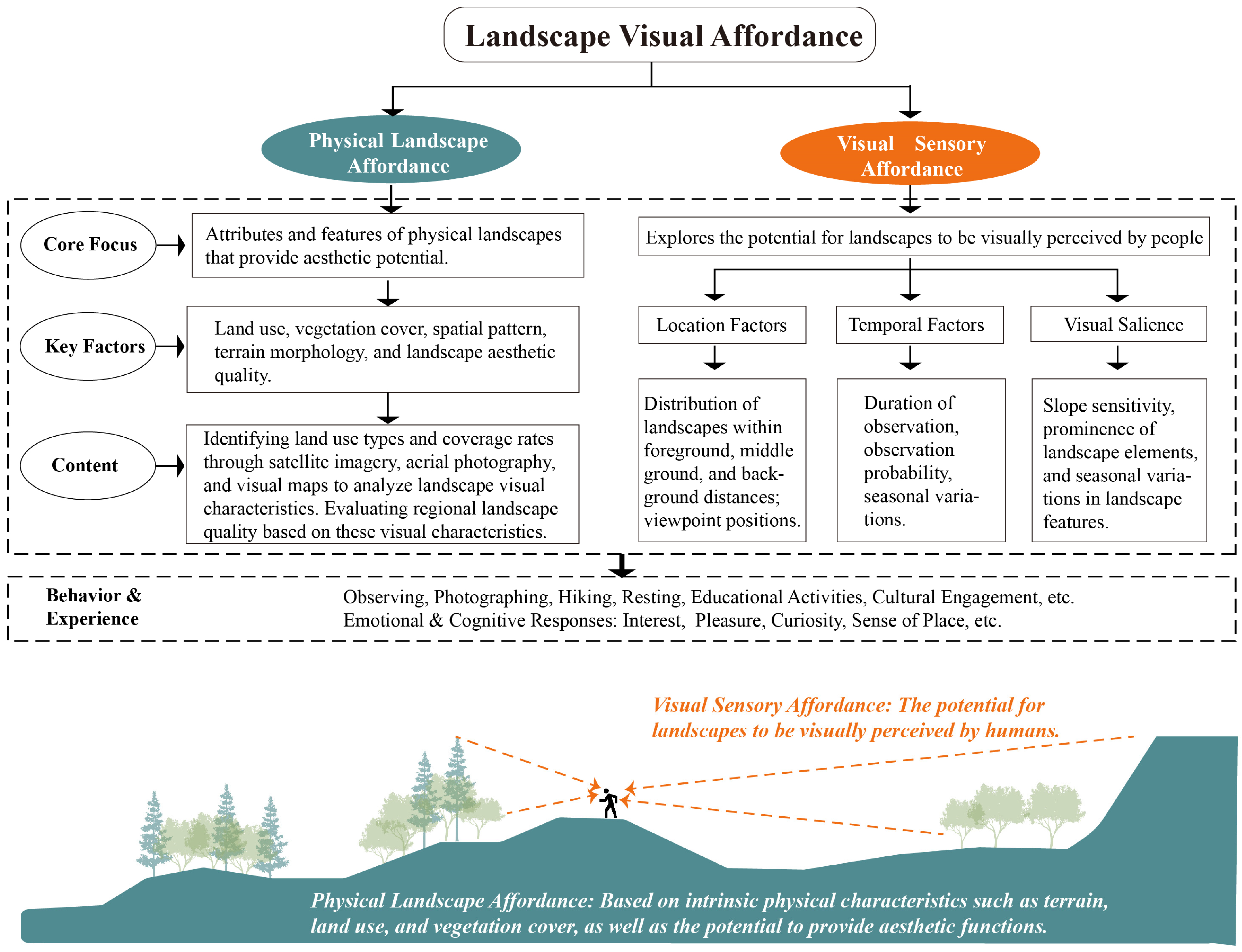
2.1. Theoretical Framework: Integrating Affordances and Visual Landscapes
2.1.1. Physical Landscape Affordance (PLA)
- Landscape visual characteristics, formed by combining the landform (slope, aspect, and general curvature), vegetation coverage (trees, shrubs, bamboo forests, nurseries, etc.), and land use types (farmland, forest land, grassland, villages, roads, water bodies, etc.) into distinct landscape patch types [31].
2.1.2. Visual Sensory Affordance (VSA)
- Location factors such as the layering of the foreground, middle ground, and background, viewpoint position and elevation, and the spatial interplay of landscape elements and potential obstructions. Research in visual ecology and environmental psychology indicates that different vantage points and distance gradients profoundly affect individuals’ sensory stimulation and aesthetic judgments [35]. Terrain, viewing distance, and barriers determine “what can be seen” and “how it is seen”, thus shaping the overall capacity for visual reception.
- Temporal factors such as viewing duration, viewing frequency, and seasonal variation. Because lighting conditions differ between day and night or during dawn and dusk, a landscape’s color, brightness, and layering are directly affected; viewing the same spot repeatedly or only briefly can produce varying degrees of visual impact and memorability. Seasonal shifts in leaf color, light intensity, and weather conditions can also alter a landscape’s appearance and aesthetic value.
- Visual salience such as color contrasts, terrain ruggedness, the diversity and seasonal dynamics of vegetation, and prominent landscape elements. The human visual system is highly sensitive to color contrasts, abrupt shapes, and distinctive landmarks. In a scenic context, striking color differences or unique landforms are more readily perceived.
- Stimulating Curiosity and a Desire to Explore: When a landscape contains multiple elements and varied boundaries (high complexity and abundant edges), visitors tend to linger, take photographs, and engage in exploration. Such visual richness can prompt extended stays, group discussions, and shared experiences.
- Immersive Experiences: Areas with high ecological integrity foster a sense of relaxation and eco-friendly tourism, enabling visitors to “escape” from urban life.
- Science Popularization and Environmental Education: Rich biodiversity or striking natural features may encourage guided tours, interpretive signage, and conservation-oriented activities.
- Contemplation and Healing: quiet, unspoiled environments and natural landscapes with minimal human interference can support meditation, health-oriented tourism, and restorative recreation.
- Cultural Tourism: Historical buildings, traditional farmland, seasonal flower fields, and distinct cultural or seasonal attributes can appeal to culture enthusiasts or “Instagram tourists”, turning certain sites into “hotspots”.
- Emotional Attachment and Local Identity: Traditional scenic resources and unique regional landscapes can enhance a sense of cultural belonging and collective memory, prompting visitors to revisit or develop a stronger place identity.
2.2. Study Area Overview
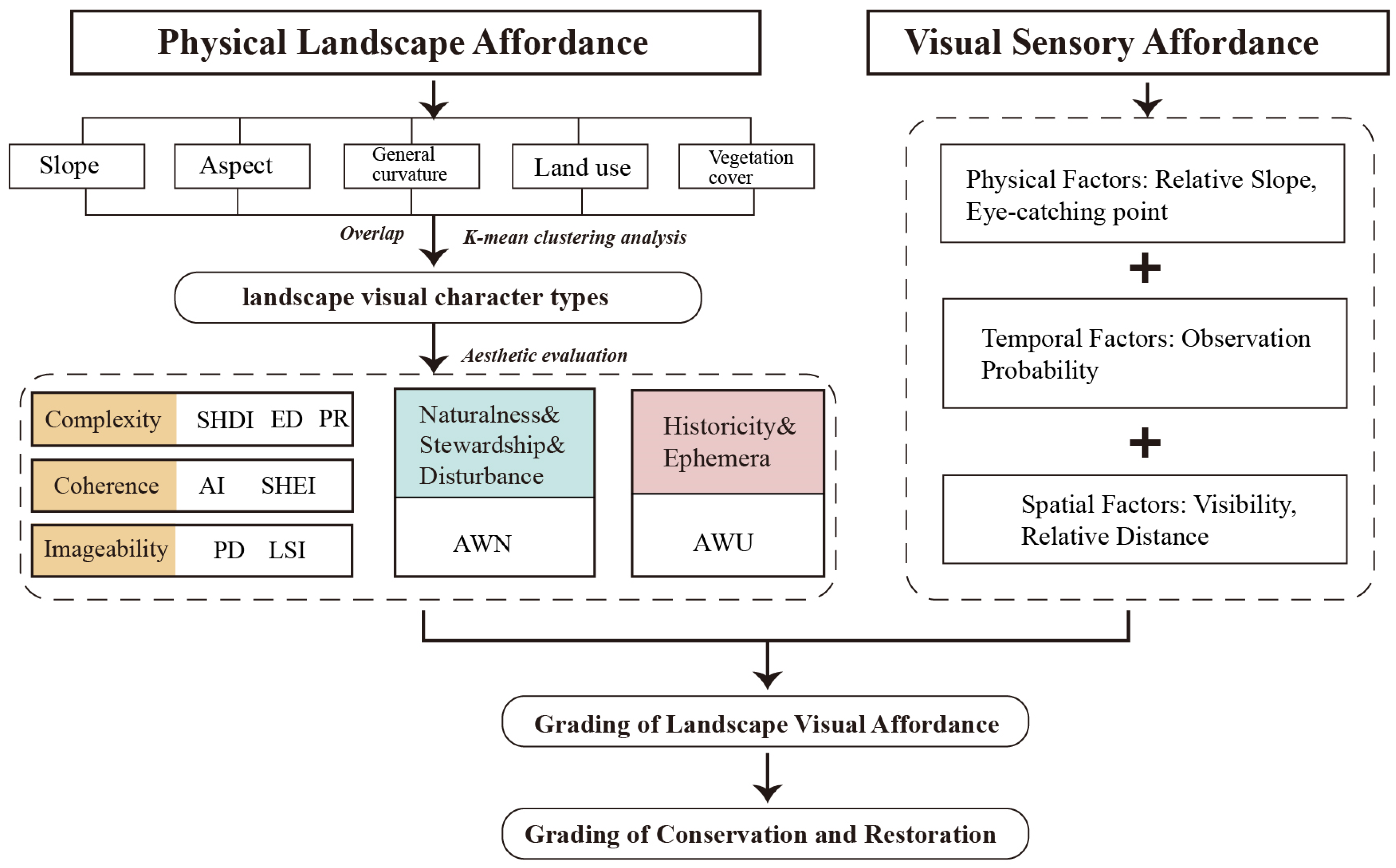
2.3. Research Framework
2.4. Aessessment of Physical Landscape Affordance
2.4.1. Assessment of Landscape Visual Characteristics
2.4.2. Aesthetic Quality Evaluation
- SHDI captures the diversity (i.e., both richness and evenness) of different patch types within a given area [44]. A higher SHDI indicates a more diversified composition of patches—such as forests, water bodies, agricultural lands, and built-up areas—and a more uniform distribution of land cover types. From a visual perspective, greater diversity in patch types tends to attract interest and engender a richer visual field. Moreover, “visual complexity” is also associated with the number of perceived edges or transitions [33]. More frequent edges or transitions can enhance the visual interest and complexity of a scene.
- ED measures the total length of patch boundaries per unit area. A higher ED implies that the spatial structure contains more patch edges, transitions, and fine-scale contrasts. Visually, abundant edges require the eye to process more “breaks” or “boundaries”, thereby contributing to the overall perception of spatial complexity [34].
- PR reflects the number of different land use types, vegetation types, or other functional units within the landscape. A higher PR indicates the presence of a greater variety of patches, and this heterogeneity directly increases the variety and stratification of visual elements, resulting in a more diverse and dynamic visual appearance that enhances visual diversity. Additionally, PR is positively correlated with a “sense of wonder”, which is a core psychological mechanism underlying imageability [11].
- Imageability requires that the landscape contains visually salient and memorable components. A higher PD generally indicates that there are more elements of differing functions or types present, offering observers a wealth of visual information that can enhance the sense of identity and uniqueness of the landscape. When PD is high, it suggests that the number of patches is large and their distribution is dense, which may lead certain patches—due to their close proximity or specific arrangement—to form distinct visual focal points or landmark features, thereby enhancing the vividness and memorability of the landscape [22].
- The LSI primarily reflects the complexity of patch boundaries and the irregularity of their shapes. The “panoramic” characteristics and “spectacular elements” of a landscape are often closely related to the complexity of its edges and the uniqueness of its shapes. Complex and distinctive forms tend to capture visual attention, forming prominent landmarks or recognizable images. A higher LSI indicates that patch shapes are complex and variable; this irregularity and complexity may enhance the visual impact of certain patches within the overall landscape, making them stand out and thus increasing the landscape’s imageability. Furthermore, complex boundaries and shapes help construct a richer visual texture, ensuring that the landscape presents a unique and attractive image from different viewing angles and distances [31,43,45].
- Very high naturalness (score 5): primarily tree-covered areas (e.g., broad-leaved forests and bamboo groves) and water bodies with minimal human interference.
- High naturalness (score 4): other forested areas with limited human activity.
- Moderate naturalness (score 3): shrublands, grasslands, and dry farmland.
- Low naturalness (score 2): irrigated paddy fields, tea plantations, orchards, and managed woodlands under more intense cultivation.
- Very low naturalness (score 1): construction land, strongly dominated by human interventions.
2.5. Assessment of Visual Sensory Affordance
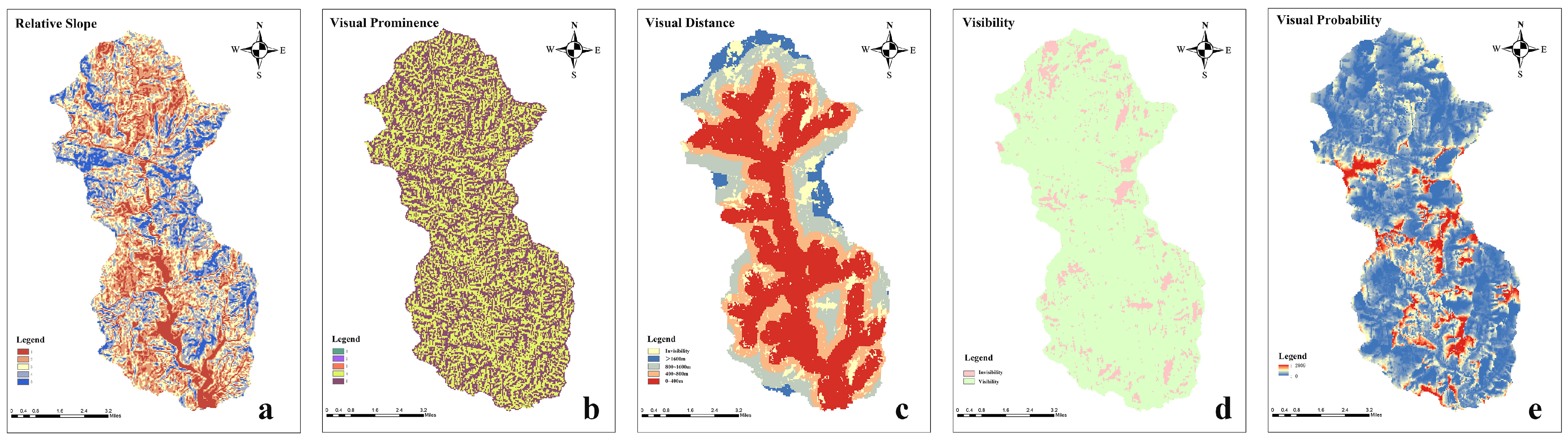
2.5.1. Visual Salience Factors: Relative Slope and Prominence
2.5.2. Location Factors: Visibility and Visual Distance
2.5.3. Temporal Factors: Visual Probability
2.5.4. Integrated Visual Sensory Affordance
3. Results
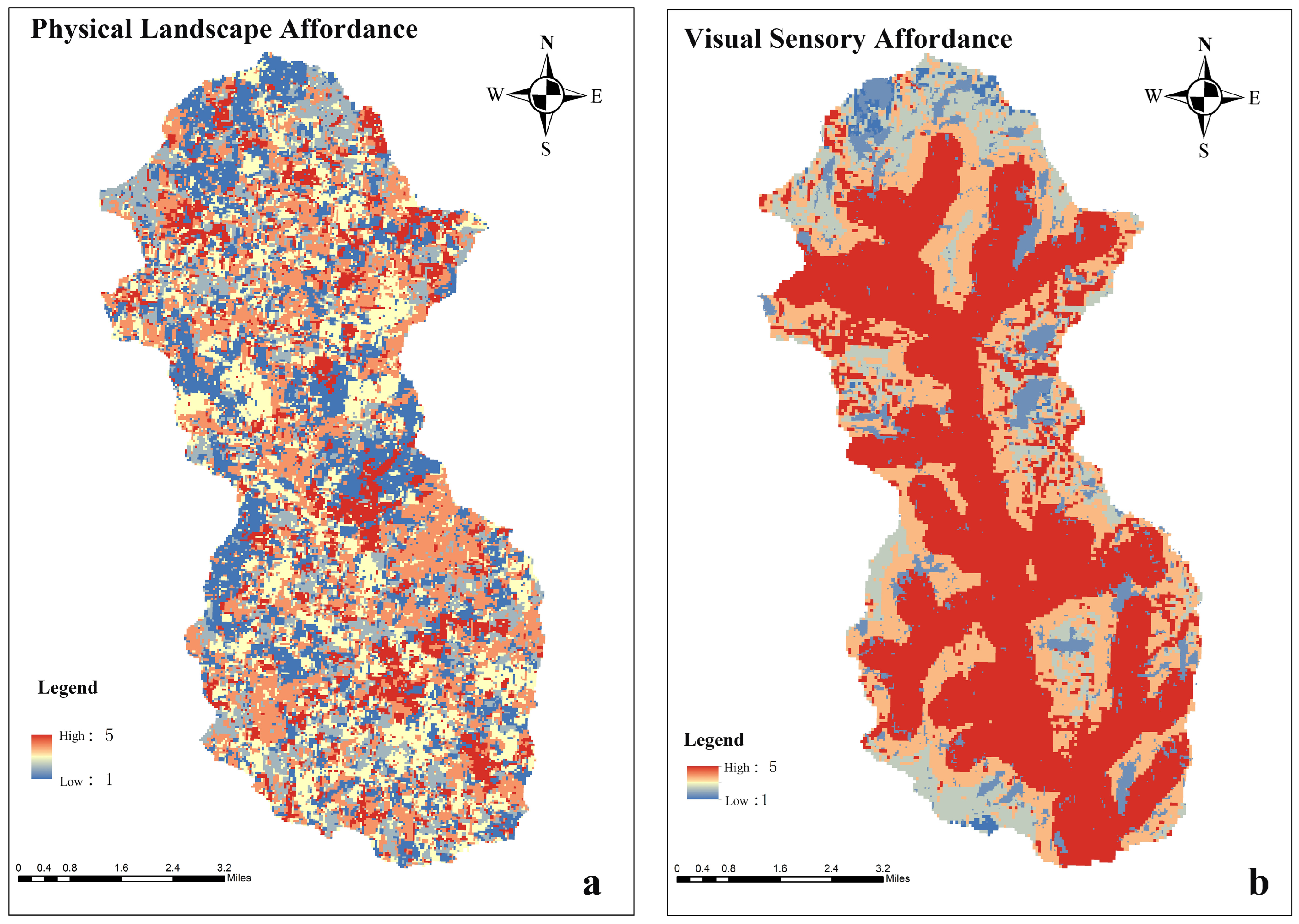
3.1. Results of Physical Landscape Affordance
3.2. Results of Visual Sensory Affordance
3.3. Comprehensive Landscape Visual Affordance
4. Discussion
4.1. Methodological Characteristics
4.2. Implications for National Park Landscape Planning and Management
- (1)
- Identifying Priority Areas for Conservation and Management. By quantifying PLA and VSA indicators, this method can effectively detect the most representative yet vulnerable sites within a national park. Regions with high LVA scores are often visually prominent and hold substantial aesthetic value, but they may also be at higher risk from ecological pressures and human disturbance. Targeted zoning measures, visitor capacity controls, and well-designed recreational infrastructure can be implemented in these “landscape hotspots” to alleviate pressures on fragile ecosystems.
- (2)
- The LVA approach enables planners to gain deeper insights into potential visual focal points. When a national park is slated to build or upgrade recreational facilities, transportation routes, or visitor centers, management must not only consider land use and ecological impacts but also evaluate how such developments might affect critical scenic corridors or key landscape nodes. LVA provides a technical basis for identifying core viewsheds and distinctive aesthetic features, informing early-stage assessments and guiding architectural siting, overall design, and harmony with the surrounding environment. In certain areas with high visual affordance, LVA results can even justify rejecting or strictly limiting construction. Different combinations of PLA and VSA not only reflect the landscape’s inherent aesthetic potential and degree of visibility but also shape visitors’ behavior and psychological experiences. By comparing PLA and VSA assessments across diverse zones and taking into account common visitor activities in national parks, we can derive the following major insights and recommendations (Table 11).
- (3)
- Facilitating Multi-Objective Management and Stakeholder Coordination. Owing to their multifunctional nature, national parks must balance ecological conservation, recreational development, and community interests. By emphasizing a landscape’s visual dimension, LVA underscores the importance of scenic value for public perception and cultural identity, offering a transparent, data-driven basis for participatory decision-making. For instance, when assessing whether a new visitor center or scenic corridor should be built, LVA analyses can visually illustrate potential impacts on the park’s overall scenic appeal and ecological sensitivity, thus helping to devise spatial layouts that respect both biodiversity conservation and social demand.
- (4)
- Balancing Visitor Perceptions with Ecological Protection. National parks are often associated with public aspirations for pristine natural environments, yet excessive visitor traffic can disrupt ecological balance. Incorporating LVA into regular monitoring and decision-making can reveal impending overloads on environmental capacities—such as trampling or landscape degradation—and trigger timely remedial measures such as dispersion or access restrictions. Through interpretive signage and visitor education, park authorities can also foster a public understanding of conservation imperatives.
4.3. Limitations and Future Directions
- Subjectivity in indicator selection: The choice of indicators stems from different conceptual frameworks and theories of visual quality, varying according to cultural norms and values [16]. As such, adopting different indicators might alter the evaluation outcomes.
- Potential discrepancies in perceived vs. potential visual quality: PLA assessments, based on geospatial data, primarily reveal the possibility or potential for a landscape to exhibit high visual quality. VSA captures the significance of a landscape’s visibility within the perception process but is not directly based on photographic interpretation. Therefore, a high-PLA area might still yield lower real-world visual quality if obstructed by elements such as unsightly power lines, discordant building colors, or excessive heights [14]. Hence, the current method is well-suited to macro-level regional planning, but local-scale planning may additionally require photo-based evaluations [4].
- Lack of dynamic and long-term monitoring: Landscape characteristics and visual elements within national parks often exhibit pronounced seasonal or climatic variability, potentially affecting LVA metrics over annual or inter-annual cycles. Future research should integrate extended temporal monitoring via remote sensing, field surveys, and visitor behavior data, allowing for the accurate assessment of LVA as landscapes evolve under environmental succession and climate change.
5. Conclusions
Author Contributions
Funding
Data Availability Statement
Conflicts of Interest
References
- Sullivan, R.G.; Meyer, M.E. Environmental Reviews and Case Studies: The National Park Service Visual Resource Inventory: Capturing the Historic and Cultural Values of Scenic Views. Environ. Pract. 2016, 18, 166–179. [Google Scholar] [CrossRef]
- Xu, L.; Yu, H. Research progress on landscape evaluation, protection and utilization of foreign national parks and its enlightenment on China. Resour. Sci. 2022, 44, 1520–1532. (In Chinese) [Google Scholar]
- Bureau of Land Management. The Use of Color for Camouflage Concealment of Facilities. Tech Note 446. Bureau of Land Management, Washington Office: Washington, DC, USA, 2015. Available online: https://blmwyomingvisual.anl.gov/docs/CamouflageBLM_TN_446.pdf (accessed on 1 April 2015).
- Sullivan, R.G.; Meyer, M. Documenting America’s scenic treasures: The National Park Service visual resource inventory. In Proceedings of the National Association of Environmental Professionals Annual Conference, Chicago, IL, USA, 11–14 April 2016. [Google Scholar]
- USFS (United States Forest Service). Landscape Aesthetics: A Handbook for Scenery Management, Agriculture Handbook Number 701; U.S. Department of Agriculture, U.S. Government Printing Office: Washington, DC, USA, 1995.
- Brown, G.; Brabyn, L. An analysis of the relationships between multiple values and physical landscapes at a regional scale using public participation GIS and landscape character classification. Landsc. Urban Plan. 2012, 107, 317–331. [Google Scholar] [CrossRef]
- Andrew, L. The Science of Scenery: How We View Scenic Beauty, What It Is, Why We Love It, and How to Measure and Map It; CreateSpace Independent Publishing Platform: Charleston, SC, USA, 2017. [Google Scholar]
- Lothian, A. Landscape and the philosophy of aesthetics: Is landscape quality inherent in the landscape or in the eye of the beholder? Landsc. Urban Plan. 1999, 44, 177–198. [Google Scholar] [CrossRef]
- Daniel, T.C. Whither scenic beauty? Visual landscape quality assessment in the 21st century. Landsc. Urban Plan. 2001, 54, 267–281. [Google Scholar] [CrossRef]
- BLM. Visual Resource Inventory, BLM Manual Handbook 8410-1, Release 8-28; U.S. Department of the Interior: Washington, DC, USA, 1986.
- Gobster, P.H.; Nassauer, J.I.; Daniel, T.C.; Fry, G. The shared landscape: What does aesthetics have to do with ecology? Landsc. Ecol. 2007, 22, 959–972. [Google Scholar] [CrossRef]
- Misthos, L.-M.; Krassanakis, V.; Merlemis, N.; Kesidis, A.L. Modeling the Visual Landscape: A Review on Approaches, Methods and Techniques. Sensors 2023, 23, 8135. [Google Scholar] [CrossRef] [PubMed]
- Roth, M.; Hildebrandt, S.; Walz, U.; Wende, W. Large-Area Empirically Based Visual Landscape Quality Assessment for Spatial Planning—A Validation Approach by Method Triangulation. Sustainability 2021, 13, 1891. [Google Scholar] [CrossRef]
- Walz, U.; Stein, C. Indicator for a monitoring of Germany’s landscape attractiveness. Ecol. Indic. 2018, 94, 64–73. [Google Scholar] [CrossRef]
- Hermes, J.; Albert, C.; von Haaren, C. Assessing the aesthetic quality of landscapes in Germany. Ecosyst. Serv. 2018, 31, 296–307. [Google Scholar] [CrossRef]
- Kalinauskas, M.; Mikša, K.; Inácio, M.; Gomes, E.; Pereira, P. Mapping and assessment of landscape aesthetic quality in Lithuania. J. Environ. Manag. 2021, 286, 112239. [Google Scholar] [CrossRef] [PubMed]
- Li, N.; Zhang, Y.Y. Evaluation of visual landscape characteristics of Helan Mountain National Nature Reserve in Ningxia from the perspective of ecological aesthetics. Acta Ecol. Sin. 2023, 43, 9177–9192. [Google Scholar] [CrossRef]
- Bibaeva, A.Y. Aesthetic Assessment of Landscapes at the Regional Level (a Case Study of the Central Ecological Zone of the Baikal Natural Territory). Geogr. Nat. Resour. 2022, 43, 182–188. [Google Scholar] [CrossRef]
- Vukomanovic, J.; Orr, B.J. Landscape Aesthetics and the Scenic Drivers of Amenity Migration in the New West: Naturalness, Visual Scale, and Complexity. Land 2014, 3, 390–413. [Google Scholar] [CrossRef]
- Schirpke, U.; Tasser, E.; Tappeiner, U. Predicting scenic beauty of mountain regions. Landsc. Urban Plan. 2013, 111, 1–12. [Google Scholar] [CrossRef]
- Roth, M.; Hildebrandt, S.; Röhner, S.; Tilk, C.; Schwarz-von Raumer, H.G.; Roser, F.; Borsdorff, M. Landscape as an Area as Perceived by People: Empirically-Based Nationwide Modelling of Scenic Landscape Quality in Germany; Wichmann Verlag: Heidelberg, Germany, 2018. [Google Scholar] [CrossRef]
- Frank, S.; Fürst, C.; Koschke, L.; Witt, A.; Makeschin, F. Assessment of landscape aesthetics—Validation of a landscape metrics-based assessment by visual estimation of the scenic beauty. Ecol. Indic. 2013, 32, 222–231. [Google Scholar] [CrossRef]
- Tara, A.; Lawson, G.; Davies, W.; Chenoweth, A.; Pratten, G. Integrating Landscape Character Assessment with Community Values in a Scenic Evaluation Methodology for Regional Landscape Planning. Land 2024, 13, 169. [Google Scholar] [CrossRef]
- Havinga, I.; Marcos, D.; Bogaart, P.W.; Hein, L.; Tuia, D. Social media and deep learning capture the aesthetic quality of the landscape. Sci. Rep. 2021, 11, 20000. [Google Scholar] [CrossRef]
- Schirpke, U.; Tappeiner, G.; Tasser, E.; Tappeiner, U. Using conjoint analysis to gain deeper insights into aesthetic landscape preferences. Ecol. Indic. 2019, 96, 202–212. [Google Scholar] [CrossRef]
- Gibson, J.J. The Ecological Approach to Visual Perception: Classic Edition; Psychology Press: New York, NY, USA, 2014. [Google Scholar] [CrossRef]
- Gu, X.; Luo, L.; Chen, H. Environmental design method based on the mechanism of affordance. J. Beijing For. Univ. (Soc. Sci. Ed.) 2017, 16, 14–20. [Google Scholar] [CrossRef]
- Heft, H. Affordances and the Body: An Intentional Analysis of Gibson’s Ecological Approach to Visual Perception. J. Theory Soc. Behav. 1989, 19, 1–30. [Google Scholar] [CrossRef]
- Heft, H. Ecological Psychology in Context: James Gibson, Roger Barker, and the Legacy of William James’s Radical Empiricism; Psychology Press: New York, NY, USA, 2001. [Google Scholar] [CrossRef]
- Heras-Escribano, M. The Philosophy of Affordances; Springer International Publishing: Cham, Switzerland, 2019; Available online: http://link.springer.com/10.1007/978-3-319-98830-6 (accessed on 5 February 2025). [CrossRef]
- Zhao, J.; Wang, R.; Luo, P.; Xing, L.; Sun, T. Visual ecology: Exploring the relationships between ecological quality and aesthetic preference. Landsc. Ecol. Eng. 2017, 13, 107–118. [Google Scholar] [CrossRef]
- Lothian, A. Visual Resource Stewardship—An International Perspective. Land 2022, 11, 451. [Google Scholar] [CrossRef]
- Ode, Å.; Tveit, M.S.; Fry, G. Capturing Landscape Visual Character Using Indicators: Touching Base with Landscape Aesthetic Theory. Landsc. Res. 2008, 33, 89–117. [Google Scholar] [CrossRef]
- Tveit, M.; Ode, Å.; Fry, G. Key concepts in a framework for analysing visual landscape character. Landsc. Res. 2006, 31, 229–255. [Google Scholar] [CrossRef]
- Smardon, R.C.; Litton, R.B. Development of Visual Activity Classification and Advanced Testing on Visual Impact Assessment Manual Procedures; SUNY College of Environmental Science and Forestry: Syracuse, NY, USA, 1981. [Google Scholar]
- Cao, Y.; Yang, P.; Xu, M.; Li, M.; Li, Y.; Guo, R. A novel method of urban landscape perception based on biological vision process. Landsc. Urban Plan. 2025, 254, 105246. [Google Scholar] [CrossRef]
- Inglis, N.C.; Vukomanovic, J.; Costanza, J.; Singh, K.K. From viewsheds to viewscapes: Trends in landscape visibility and visual quality research. Landsc. Urban Plan. 2022, 224, 104424. [Google Scholar] [CrossRef]
- Zhou, L.; Zhao, Y.; Yang, X.; He, J.; Wang, H. Identification of important terraced visual landscapes based on a sensitivity-subjectivity preference matrix for agricultural cultural heritage in the southwestern china. Ecol. Indic. 2023, 154, 110573. [Google Scholar] [CrossRef]
- Chander, G.; Markham, B. Revised landsat-5 tm radiometric calibration procedures and postcalibration dynamic ranges. IEEE Trans. Geosci. Remote Sens. 2003, 41, 2674–2677. [Google Scholar] [CrossRef]
- Hantson, S.; Chuvieco, E. Evaluation of different topographic correction methods for Landsat imagery. Int. J. Appl. Earth Obs. Geoinf. 2011, 13, 691–700. [Google Scholar] [CrossRef]
- Vicenteserrano, S.; Perezcabello, F.; Lasanta, T.; Vicente-Serrano, S.M. Assessment of radiometric correction techniques in analyzing vegetation variability and change using time series of Landsat images. Remote Sens. Environ. 2008, 112, 3916–3934. [Google Scholar] [CrossRef]
- Yang, D. Study on Multi-Scale Landscape Character Types and Regional Identification. Doctoral Dissertation, Huazhong Agricultural University, Wuhan, China.
- Fry, G.; Tveit, M.S.; Ode, A.; Velarde, M.D. The ecology of visual landscapes: Exploring the conceptual common ground of visual and ecological landscape indicators. Ecol. Indic. 2009, 9, 933–947. [Google Scholar] [CrossRef]
- Turner, M.G. Landscape Ecology in Theory and Practice: Pattern and Process; Springer: New York, NY, USA, 2001. [Google Scholar]
- Sheremet, E.; Kalutskova, N.; Dekhnich, V. Visual characteristics of landscapes and methods for their assessment on GIS (Belogradchik rocks (Bulgaria) as an example). InterCarto. InterGIS 2021, 27, 191–204. [Google Scholar] [CrossRef]
- Bornstein, M.H.; Gibson, J.J. The Ecological Approach to Visual Perception. J. Aesthet. Art Crit. 1980, 39, 203. Available online: https://www.jstor.org/stable/10.2307/429816?origin=crossref (accessed on 24 August 2024). [CrossRef]
- Arthur, L.M.; Daniel, T.C.; Boster, R.S. Scenic assessment: An overview. Landsc. Plan. 1977, 4, 109–129. [Google Scholar] [CrossRef]
- Junge, X.; Schüpbach, B.; Walter, T.; Schmid, B.; Lindemann-Matthies, P. Aesthetic quality of agricultural landscape elements in different seasonal stages in Switzerland. Landsc. Urban Plan. 2015, 133, 67–77. [Google Scholar] [CrossRef]
- Qi, J.; Zhou, Y.; Zeng, L.; Tang, X. Aesthetic heterogeneity on rural landscape: Pathway discrepancy between perception and cognition. J. Rural. Stud. 2022, 92, 383–394. [Google Scholar] [CrossRef]
- Uuemaa, E.; Antrop, M.; Roosaare, J.; Marja, R.; Mander, U. Landscape Metrics and Indices: An Overview of Their Use in Landscape Research. Living Rev. Landsc. Res. 2009, 3, 1–28. [Google Scholar] [CrossRef]
- Ode, Å.; Fry, G.; Tveit, M.S.; Messager, P.; Miller, D. Indicators of perceived naturalness as drivers of landscape preference. J. Environ. Manag. 2009, 90, 375–383. [Google Scholar] [CrossRef]
- Myadzelets, A.V. Historical-cultural education functions of geosystems of specially protected nature areas on the example of the Pribaikalsky National Park. IOP Conf. Ser. Earth Environ. Sci. 2021, 885, 012059. [Google Scholar] [CrossRef]


| Category | Classification Basis | Classification |
|---|---|---|
| Slope | Natural Breaks | Gentle Slope (0°~5°), Mild Slope (5°~10°), Moderate Slope (10°~15°), Medium Slope (15°~25°), Steep Slope (25°~30°), Steeper Slope (30°~45°), Extremely Steep Slope (>45°) |
| Aspect | Sun Position | Flat (−1°), Shadowed Area (0°~45°, 315°~360°), Semi-Shadowed Area (45°~135°), Sunlit Area (135°~225°), Semi-Sunlit Area (225°~315°) |
| General Curvature | Topography | Valley (<0 m−1), Range (>0 m−1) |
| Land Use | Visual Characteristics | Forest, Grassland, Built Area, Farmland, Orchard, Water Area, Swamp, Forest Land, Bamboo, Tea Garden |
| Vegetation Cover | Type Name | Forest, Unplanted Area, Special Woodland, Agricultural Plantation, Bamboo, Shrubs, General Timberland, Nursery, Burned Area, Other |
| Visual Character Concept | Definition [15,16] | Indicators | Calculation Method | Potential Behaviors/Psychological Experiences |
|---|---|---|---|---|
| Complexity | Diversity and richness of landscape element types and boundaries. | SHDI | where Pi is the proportion of each land cover type, and R is the total number of land cover types. |
|
| ED | where E is the total length of edges between different patch types, and A is the total landscape area. | |||
| PR | The total number of different patch types within a landscape. | |||
| Imageability | Strong visual imagery conveyed by a combination of one or more landscape elements, making the landscape identifiable. | PD | where PN is the number of patches, and A is the total area. |
|
| LSI | where P is the perimeter of the patch, and A is the area of the patch. | |||
| Coherence | Aggregation of similar landscape elements in space and the balance between different elements. Coherence involves not only aggregation but also coordination and balance. | AI | where is the number of like adjacencies (joins) between pixels of patch type i, and is the maximum possible number of like adjacencies. | Comfort and Relaxation: Landscapes with a high degree of coherence or balance can foster a sense of “visual calm” and emotional relief, encouraging visitors to rest or daydream. |
| SHEI | Where is the proportion of the i-th type (e.g, species or land cover type) relative to the total number, and R is the total number of types (e.g., total number of species or patch types). | |||
| Stewardship and Disturbance and naturalness | The gradient of natural perception resulting from human intervention and management reflects a continuum ranging from entirely natural to highly artificial states. | AWN | where is the percentage of type in the landscape, is the assigned naturalness value of type , and is the area of patch . |
|
| Historicityand Ephemera | Assessment of cultural elements with varying temporal scales, as well as elements and land cover types that change with seasonal and weather variations. | AWU | where AWU is the Area-weighted uniqueness; is the Uniqueness value assigned to type ; and is the Proportion of type within the landscape. |
|
| PLA Level | Count | Area (km2) | Account (%) |
|---|---|---|---|
| 1 | 13,722 | 32.9617 | 23.92 |
| 2 | 8485 | 20.3818 | 14.79 |
| 3 | 12,868 | 30.9103 | 22.43 |
| 4 | 14,903 | 35.7986 | 25.98 |
| 5 | 7387 | 17.7443 | 12.88 |
| Classification | Relative Slope | Account (%) | Area (km2) |
|---|---|---|---|
| 1 | Gentle slopes (0°–5°) | 13.93 | 18.5703 |
| 2 | Mild slopes (5°–15°) | 26.48 | 35.2973 |
| 3 | Moderate slopes (15°–30°) | 28.45 | 37.9252 |
| 4 | Steep slopes (30°–45°) | 20.88 | 27.8250 |
| 5 | Extremely Steep Slopes (>45°) | 10.26 | 13.6725 |
| Classification | Account (%) | Area (km2) |
|---|---|---|
| 1 | 00.01 | 0.020312 |
| 2 | 00.11 | 0.14980 |
| 3 | 00.31 | 0.4163 |
| 4 | 50.58 | 68.7945 |
| 5 | 48.99 | 66.6388 |
| Classification | Visibility and Visual Distance | Account (%) | AREA (km2) |
|---|---|---|---|
| 1 | Invisibility | 9.86 | 13.3831 |
| 2 | Distant background (>1600 m) | 6.18 | 8.3904 |
| 3 | Background (800–1600 m) | 12.94 | 17.5636 |
| 4 | Middle ground (400–800 m), | 26.47 | 35.9322 |
| 5 | Foreground (0–400 m) | 44.55 | 60.4683 |
| Classification | Frequency of Being Seen | Account (%) | AREA (km2) |
|---|---|---|---|
| 1 | 0–120 | 91.38 | 124.0636 |
| 2 | 120–310 | 7.63 | 10.3617 |
| 3 | 310–580 | 0.84 | 1.1450 |
| 4 | 580–1000 | 0.11 | 0.1548 |
| 5 | 1000–2809 | 00.03 | 0.0355 |
| VSA-Level | Account (%) | AREA (km2) |
|---|---|---|
| 1 | 6.86 | 9.1494 |
| 2 | 4.61 | 6.1485 |
| 3 | 13.61 | 18.1453 |
| 4 | 30.81 | 41.0923 |
| 5 | 44.11 | 58.8309 |
| Account (%) | Area (km2) | LVCT | PLA-MEAN | VSA-MEAN | LVA-MEAN | |
|---|---|---|---|---|---|---|
| 1 | 0.0240 | 0.0330 | Gentle Slope Valley Broadleaf Forest | 3.0714 | 4.3333 | 3.1667 |
| 2 | 0.0848 | 0.1169 | Mild Slope Shaded Valley Broadleaf Forest | 3.2500 | 4.2381 | 3.6111 |
| 3 | 0.4590 | 0.6328 | Mild Slope Shaded Valley Shrubland | 2.8197 | 4.2621 | 3.6387 |
| 4 | 5.3955 | 7.4388 | Moderate Slope Shaded Valley Broadleaf Forest | 2.8983 | 4.2165 | 3.5691 |
| 5 | 25.3369 | 34.9321 | Moderately Steep Slope Semi-Shaded Valley Broadleaf Forest | 2.7718 | 4.2226 | 3.5030 |
| 6 | 37.2394 | 51.3423 | Steep Slope Semi-Sunny Valley Broadleaf Forest | 2.9745 | 4.2937 | 3.6378 |
| 7 | 18.9294 | 26.0981 | Steep Slope Semi-Sunny Ridge Broadleaf Forest | 2.9135 | 4.5236 | 3.6981 |
| 8 | 7.2149 | 9.9472 | Moderately Steep Slope Sunny Valley Broadleaf Forest with Paddy Fields | 2.8587 | 4.7500 | 3.7927 |
| 9 | 2.6268 | 3.6215 | Moderately Steep Slope Semi-Sunny Valley Special Shrubland with Paddy Fields | 2.9220 | 4.6870 | 3.8160 |
| 10 | 2.2305 | 3.0751 | Moderately Steep Slope Sunny Valley Broadleaf Forest with Other Woodland | 2.9443 | 4.7937 | 3.8691 |
| 11 | 0.0903 | 0.1245 | Moderately Steep Slope Semi-Sunny Valley Shrubland with Villages | 3.2745 | 5.0000 | 3.8214 |
| 12 | 0.0277 | 0.0381 | Mild Slope Sunny Valley Bamboo Forest with Villages | 2.8667 | 5.0000 | 3.9545 |
| 13 | 0.0406 | 0.0559 | Mild Slope Sunny Valley Broadleaf Forest with Villages | 3.0000 | 5.0000 | 4.1000 |
| 14 | 0.0774 | 0.1067 | Moderate Slope Sunny Valley Shrubland with Villages | 2.8095 | 5.0000 | 3.9545 |
| 15 | 0.0719 | 0.0991 | Moderately Steep Slope Semi-Sunny Valley Broadleaf Forest with Villages | 2.7879 | 5.0000 | 4.0526 |
| 16 | 0.0811 | 0.1118 | Mild Slope Semi-Sunny Valley Water Area | 3.3415 | 5.0000 | 4.1765 |
| 17 | 0.0350 | 0.0482 | Mild Slope Semi-Shaded Valley Water Area | 2.5882 | 5.0000 | 4.0000 |
| 18 | 0.0018 | 0.0025 | Mild Slope Semi-Sunny Ridge Water Area | 2.5000 | 5.0000 | 3.0000 |
| 19 | 0.0111 | 0.0152 | Moderately Steep Slope Semi-Sunny Valley Water Area | 1.8333 | 5.0000 | 4.5000 |
| 20 | 0.0221 | 0.0304 | Moderately Steep Slope Semi-Sunny Valley Broadleaf Forest with Water Area | 3.0833 | 5.0000 | 3.7500 |
| LVA | Account (%) | Count | Area (km2) |
|---|---|---|---|
| 1 | 11.00 | 2857 | 14.8792 |
| 2 | 22.47 | 5838 | 30.4043 |
| 3 | 18.78 | 4879 | 25.4099 |
| 4 | 22.16 | 5757 | 29.9825 |
| 5 | 25.60 | 6650 | 34.6332 |
| Category | Landscape Characteristics | Potential Visitor Behaviors/Psychological Experiences | Planning and Management Strategies |
|---|---|---|---|
| High PLA and High VSA |
|
|
|
| High PLA and Low VSA |
|
|
|
| Low PLA and High VSA |
|
|
|
| Low PLA and Low VSA |
|
|
|
Disclaimer/Publisher’s Note: The statements, opinions and data contained in all publications are solely those of the individual author(s) and contributor(s) and not of MDPI and/or the editor(s). MDPI and/or the editor(s) disclaim responsibility for any injury to people or property resulting from any ideas, methods, instructions or products referred to in the content. |
© 2025 by the authors. Licensee MDPI, Basel, Switzerland. This article is an open access article distributed under the terms and conditions of the Creative Commons Attribution (CC BY) license (https://creativecommons.org/licenses/by/4.0/).
Share and Cite
Dong, Y.; Kang, Y.; Wu, C. Landscape Visual Affordance Evaluation at a Regional Scale in National Parks: A Case Study of the Changhong Area in Qianjiangyuan National Park. Land 2025, 14, 589. https://doi.org/10.3390/land14030589
Dong Y, Kang Y, Wu C. Landscape Visual Affordance Evaluation at a Regional Scale in National Parks: A Case Study of the Changhong Area in Qianjiangyuan National Park. Land. 2025; 14(3):589. https://doi.org/10.3390/land14030589
Chicago/Turabian StyleDong, Yuchen, Yuan Kang, and Chengzhao Wu. 2025. "Landscape Visual Affordance Evaluation at a Regional Scale in National Parks: A Case Study of the Changhong Area in Qianjiangyuan National Park" Land 14, no. 3: 589. https://doi.org/10.3390/land14030589
APA StyleDong, Y., Kang, Y., & Wu, C. (2025). Landscape Visual Affordance Evaluation at a Regional Scale in National Parks: A Case Study of the Changhong Area in Qianjiangyuan National Park. Land, 14(3), 589. https://doi.org/10.3390/land14030589