
Enhancing Ecological Network Connectivity Through Urban–Rural Gradient Zoning Optimization of Ecological Process Flow


Abstract

1. Introduction
2. Materials and Methods
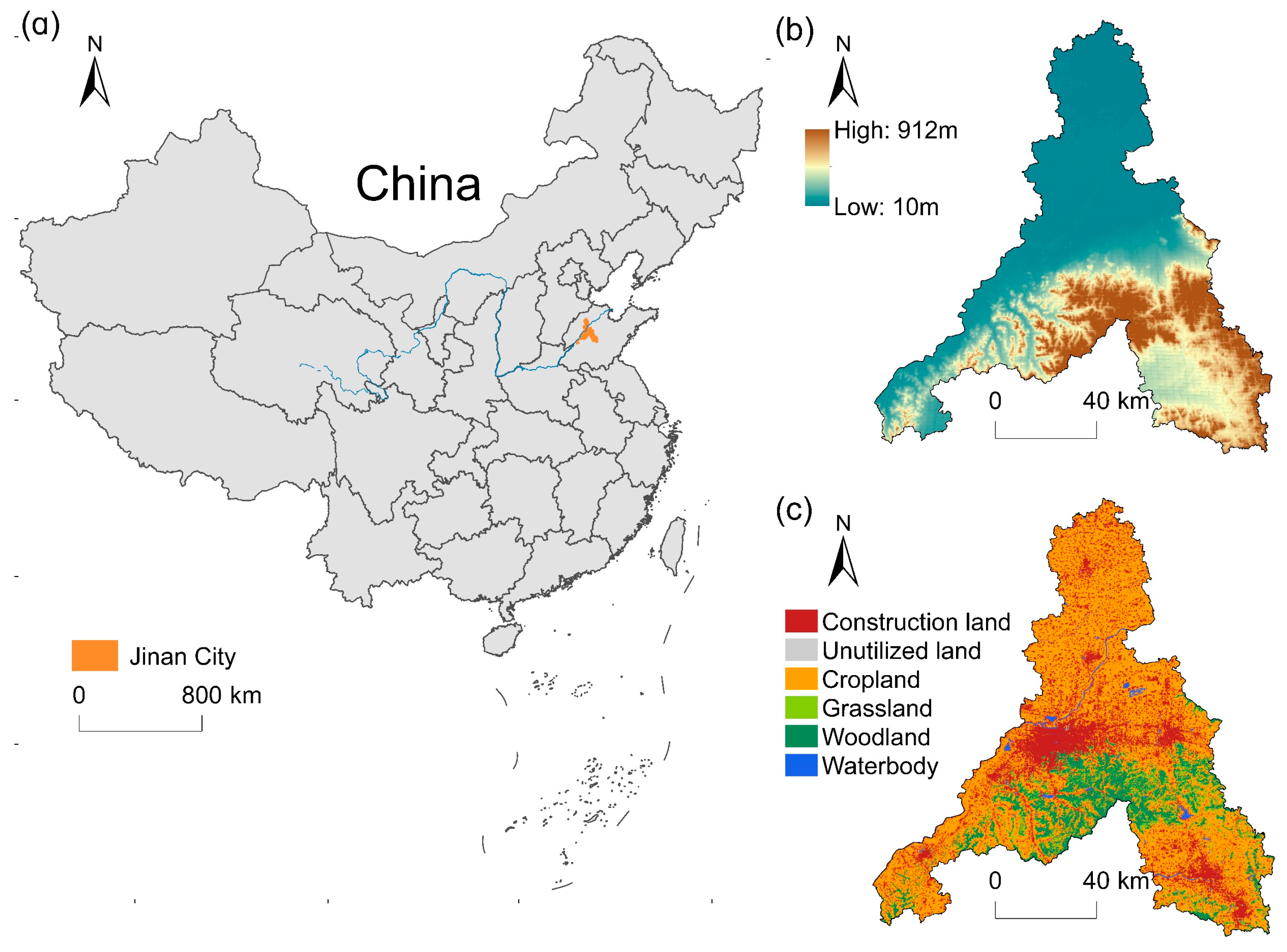
2.1. Study Area
2.2. Data Sources
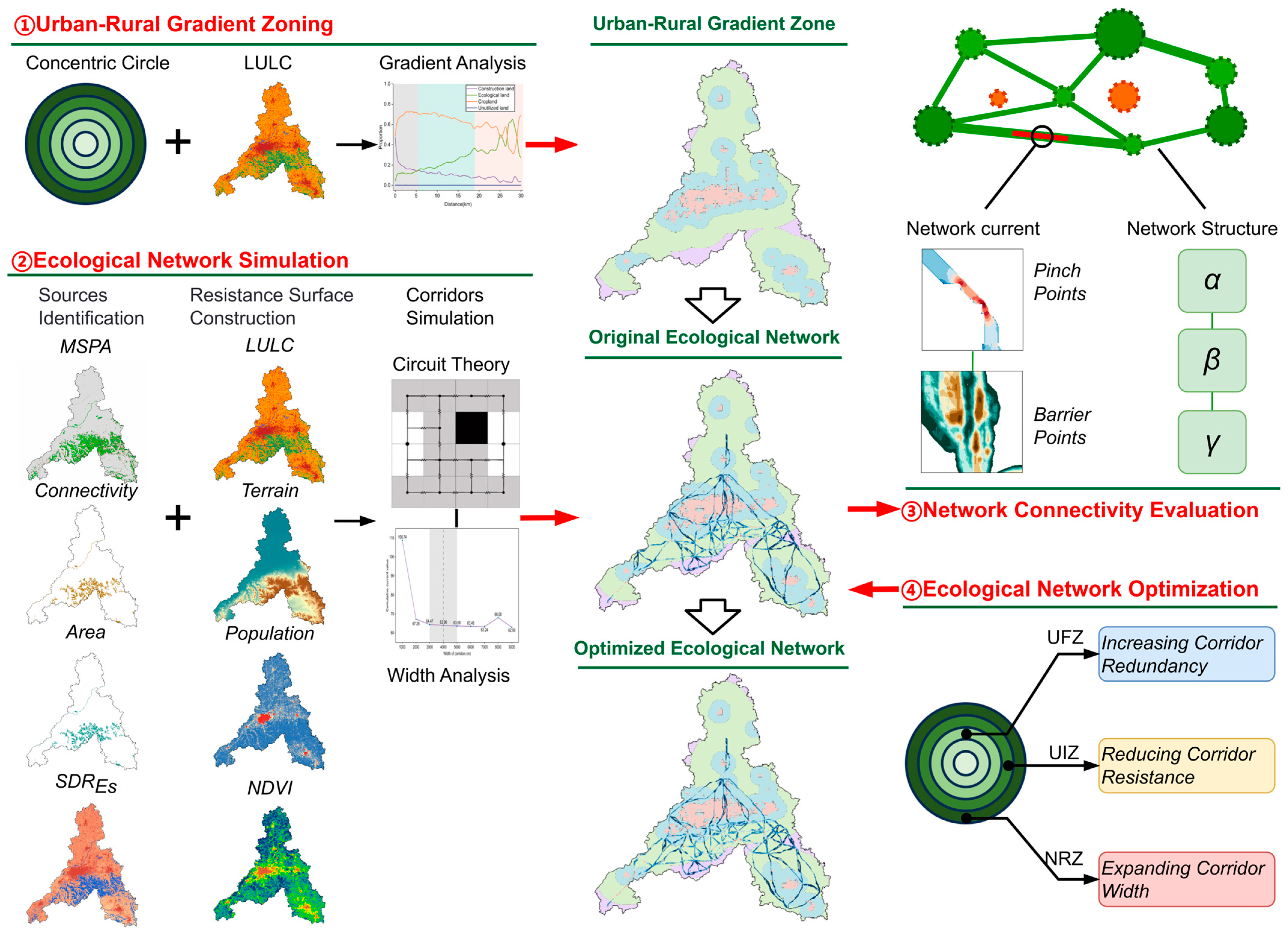
2.3. Methods
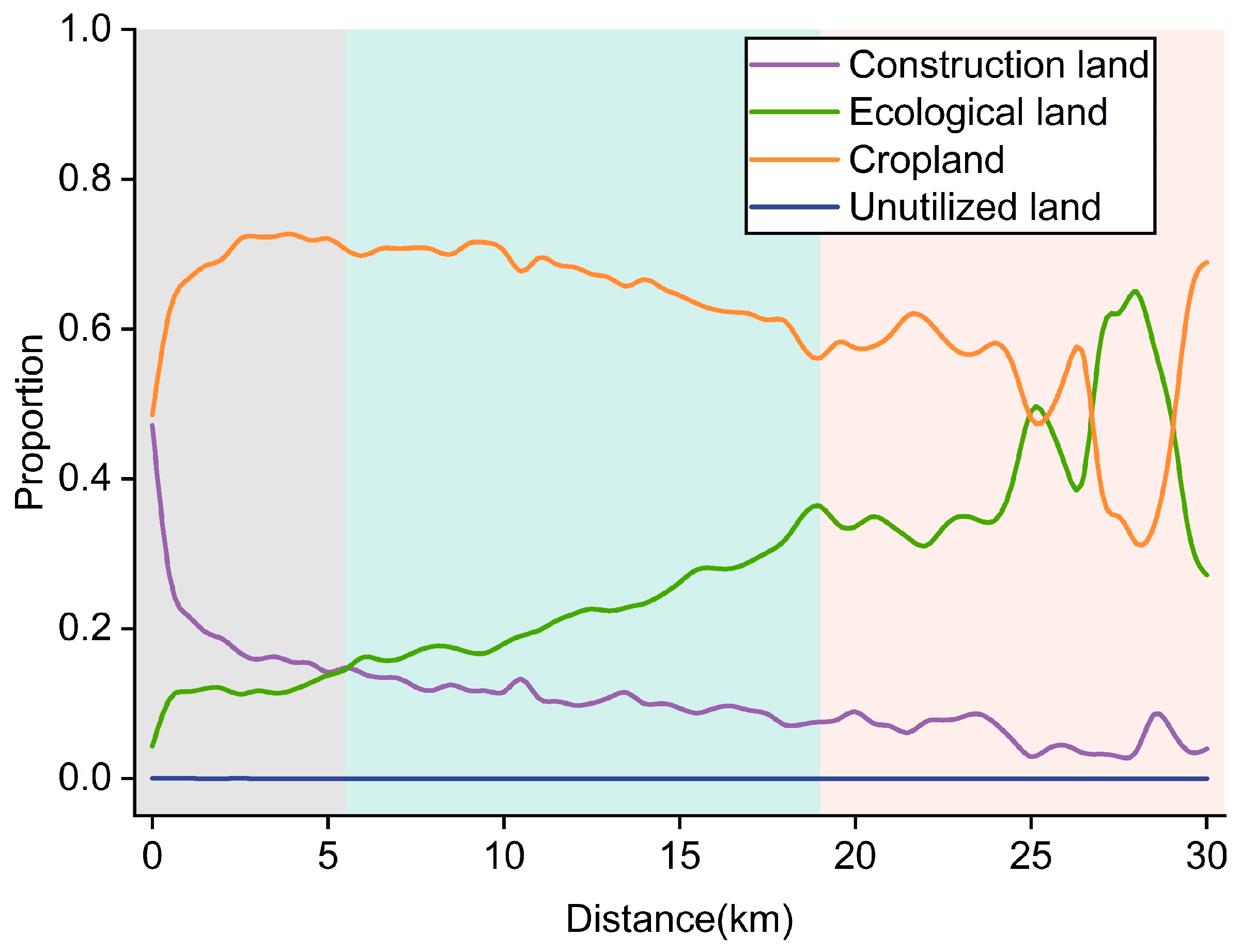
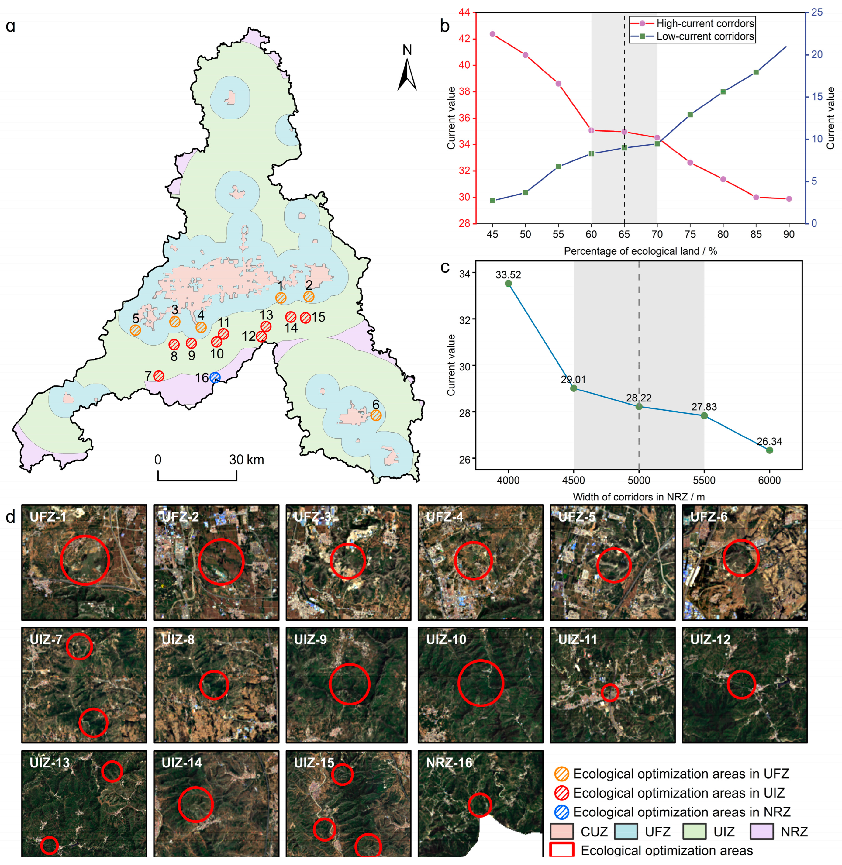
2.3.1. Urban–Rural Gradient Zoning
2.3.2. Identification of Ecological Sources
2.3.3. Construction of Ecological Resistance Surface
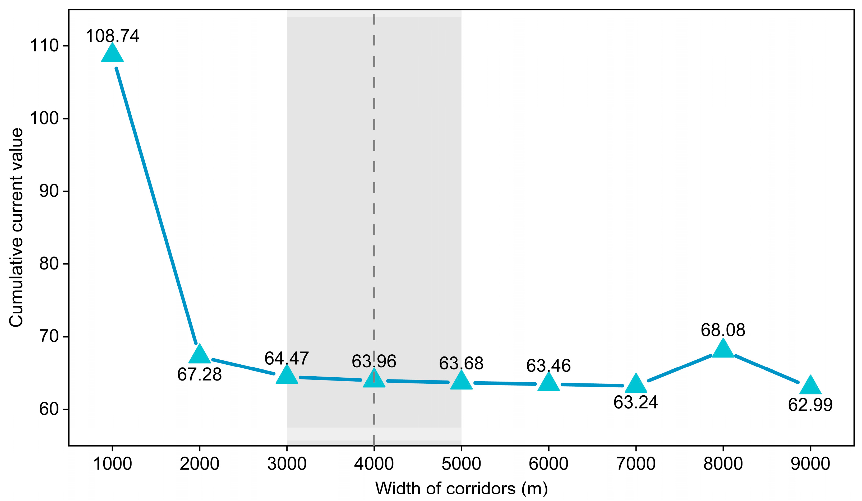
2.3.4. Simulation of Ecological Corridors
2.3.5. Evaluation of Ecological Network Connectivity
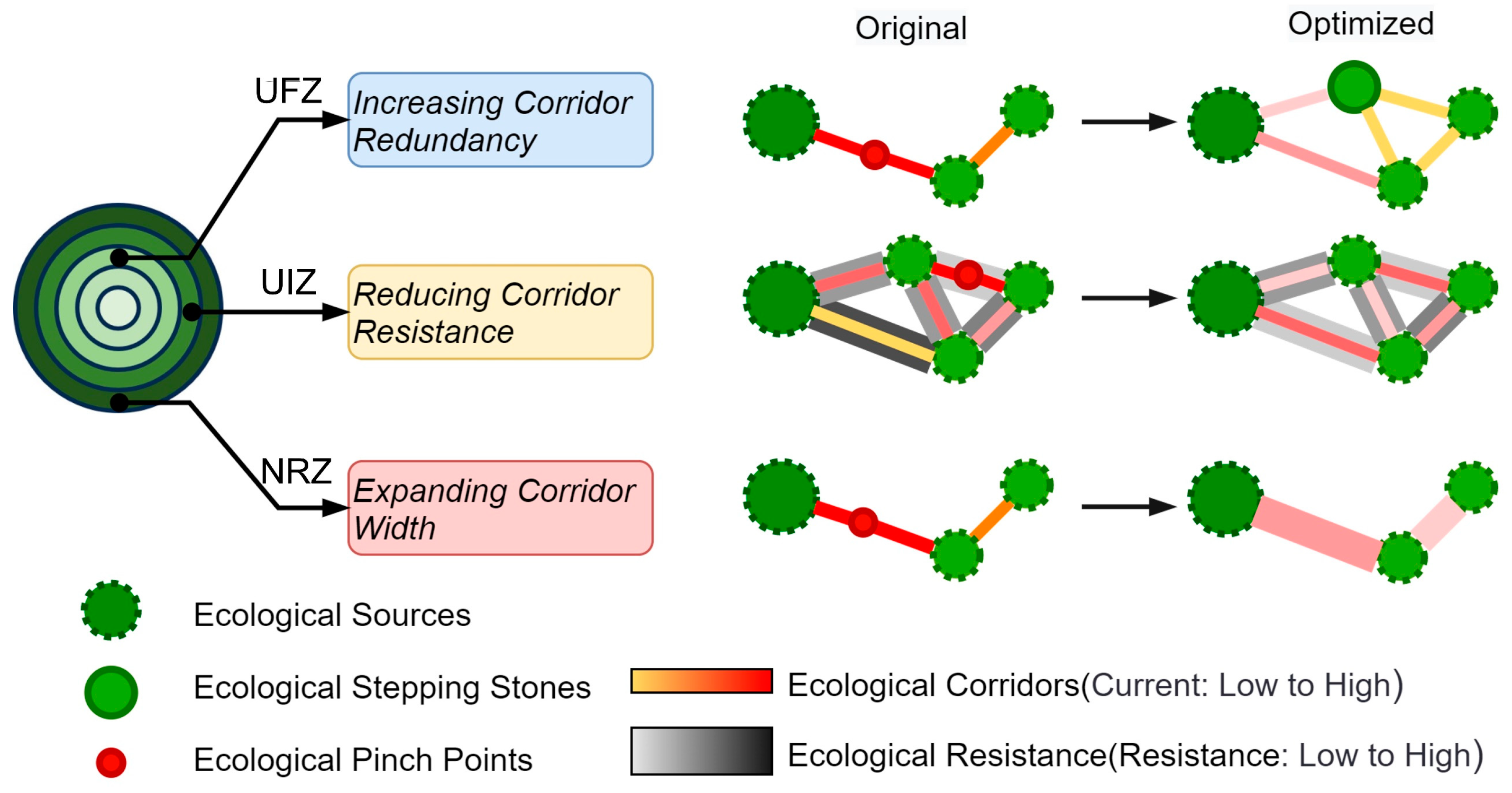
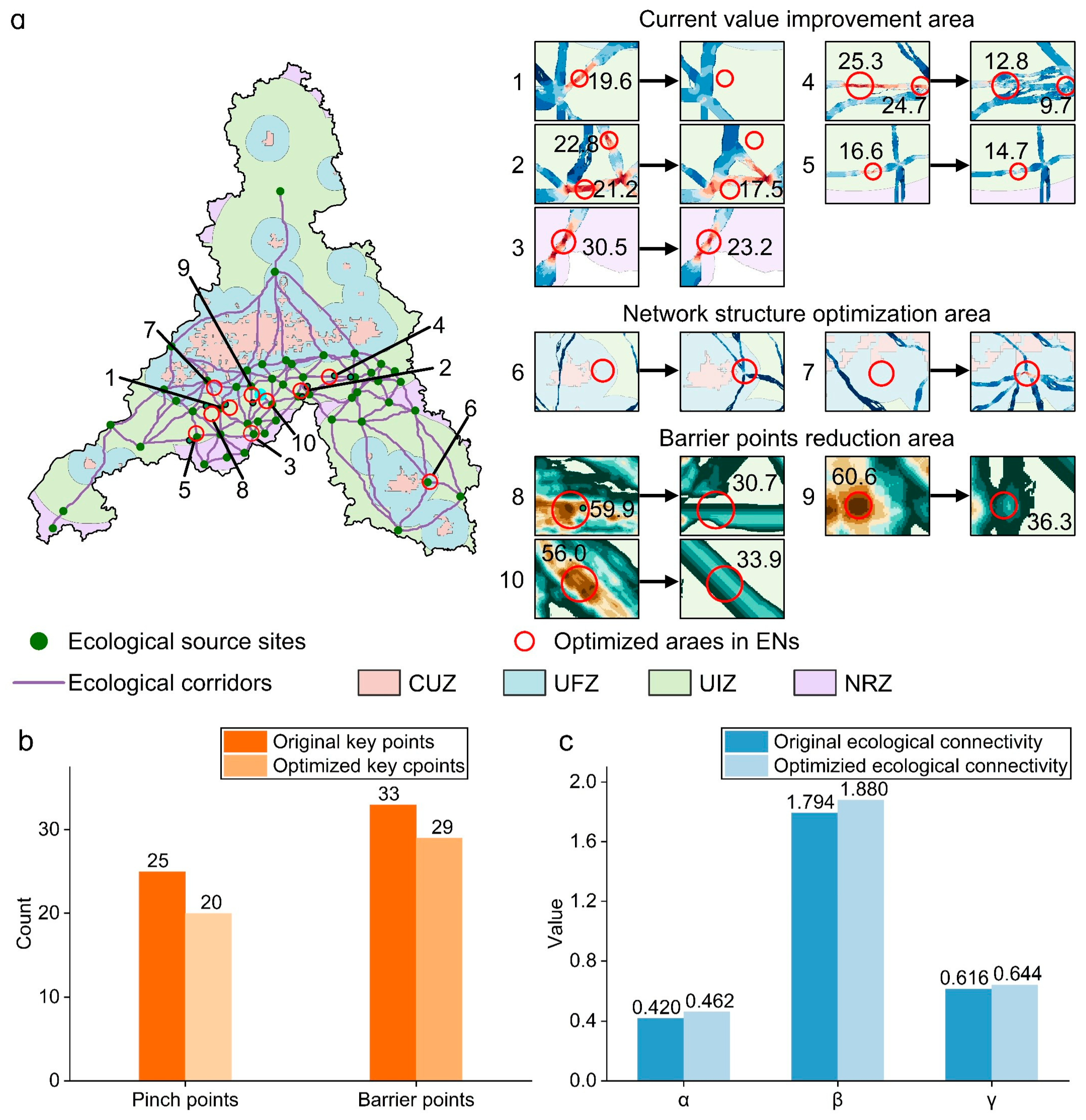
2.3.6. Ecological Networks Optimization Framework
- ➢
- UFZ: Increasing corridor redundancy
- ➢
- UIZ: Reducing corridor resistance
- ➢
- NRZ: Expanding corridor width
3. Results
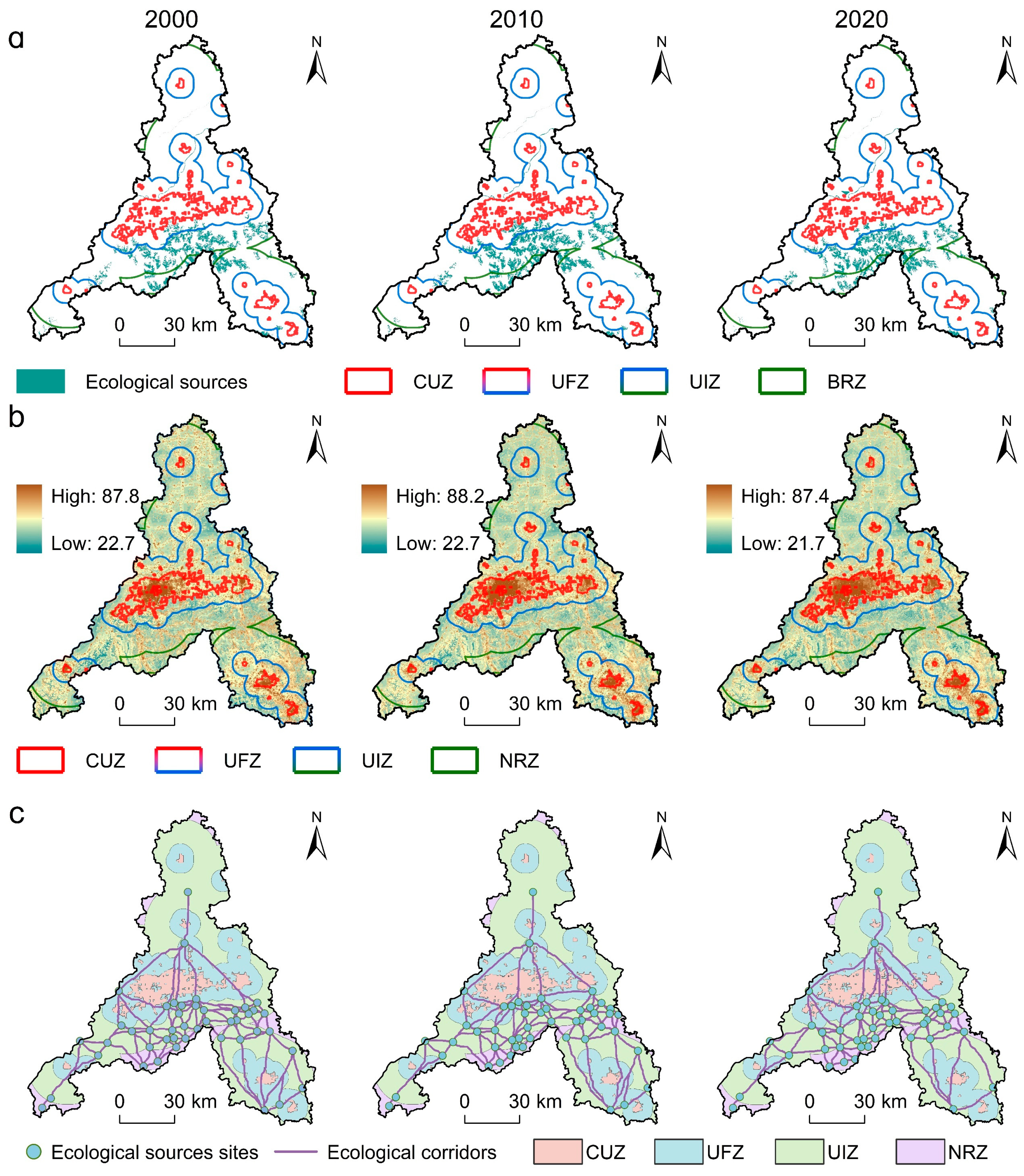
3.1. Spatio-Temporal Pattern Evolution of Ecological Networks
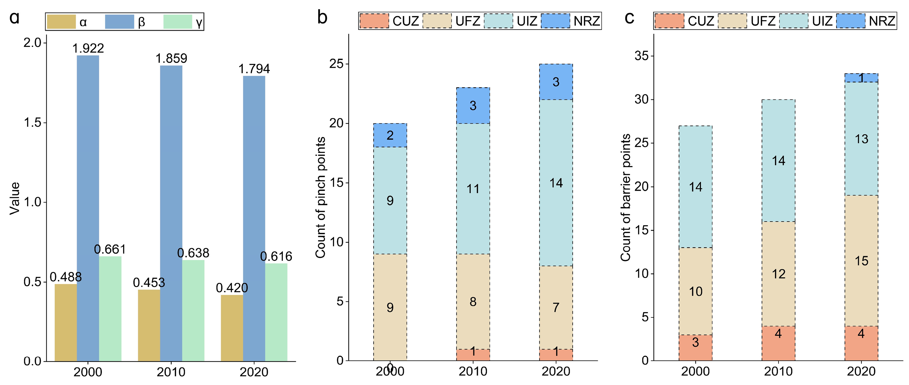
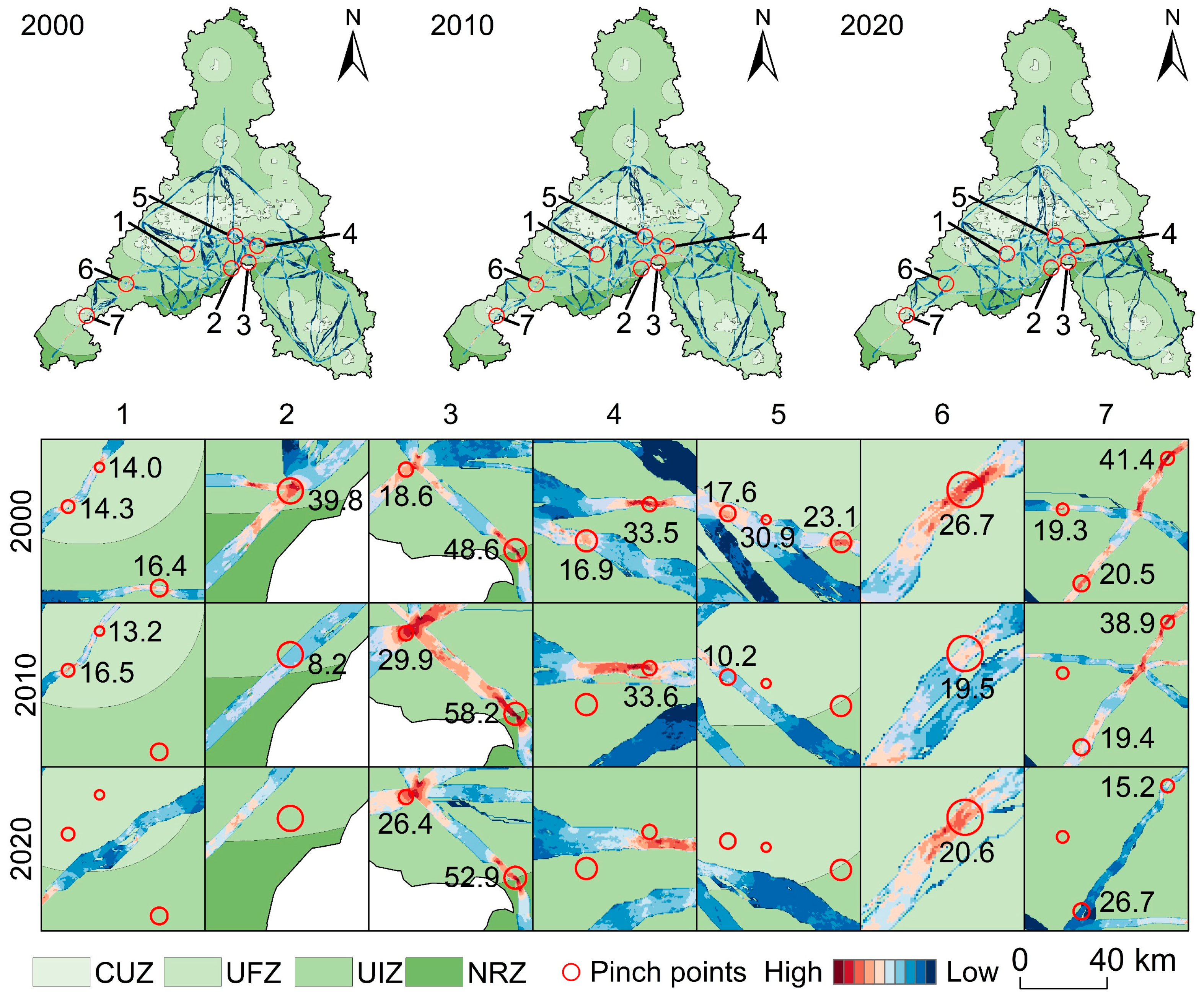
3.2. Spatio-Temporal Pattern Evolution of EN Connectivity
3.3. EN Optimization and Validation
4. Discussion
4.1. Impact of Urbanization on Ecological Connectivity and Its Countermeasures
4.2. Advantages of the Proposed EN Optimization Framework
4.3. Limitations and Future Work
5. Conclusions
Author Contributions
Funding
Data Availability Statement
Acknowledgments
Conflicts of Interest
Appendix A

| Indicators | Formulas and Meanings | ||
|---|---|---|---|
| Water Conservation | Supply function | (A1) | |
| where represents the annual average water retention capacity, which signifies water conservation supply. represents the flow velocity coefficient, represents the terrain index, represents the soil saturated hydraulic conductivity, and represents the water yield per unit grid (calculated by the water yield module of the Invest model), | |||
| Demand function | (A2) | ||
| (A3) | |||
| where represents the water resource usage demand per unit grid, which indicates the demand capacity for water resource services. represents the per capita water consumption, represents the population within a unit grid, represents the total annual water consumption, and represents the total population. | |||
| Carbon Sequestration | Supply function | (A4) | |
| where represents the total carbon supply in a unit grid, which is carbon sequestration supply. represents the total net primary productivity in a unit grid. | |||
| Demand function | (A5) | ||
| (A6) | |||
| (A7) | |||
| where represents the total carbon emissions. l represents the total electricity consumption, including residential, industrial, and agricultural electricity data for the entire society. represents the carbon emission coefficient. represents the total population. represents the per capita carbon emissions. represents the population count in a unit grid. represents the carbon emissions in a unit grid, which represents carbon sequestration demand services. | |||
| Soil Conservation | Supply function | (A8) | |
| where represents the annual average soil conservation amount, represents the rainfall erosivity factor, represents the soil erodibility factor (calculated based on the percentage of silt, sand, clay, and organic matter in the soil), represents the topographic factor, represents the crop management factor, and represents the conservation practice factor. | |||
| Demand function | InVEST model SDR module | ||
| Habitat Quality | Supply function | InVEST model habitat quality module | |
| Demand function | (A9) | ||
| where represents the habitat quality demand, represents the habitat quality supply index, which is the habitat quality supply capacity calculated based on Invest, and represents the habitat quality demand standard. | |||
| Landscape connectivity | (A10) | ||
| (A11) | |||
| where represents the total number of landscape patches, and and represent the areas of patches and , respectively. is the total landscape area of the study region. represents the maximum product of probabilities for all paths between patch and . represents the potential connectivity of landscape patches, and represents the potential connectivity of the remaining patches after removing a certain. | |||
| Ecological supply–demand ratio | . | (A12) | |
| In this equation, represents the supply–demand ratio within a single grid, represents the supply function of per grid, and represents the demand function of per grid. When > 0, it indicates that the supply of within the unit grid exceeds the demand, suggesting a surplus in supply and the absence of supply–demand imbalance. When = 0, it indicates that the supply within the unit grid exactly meets the demand, resulting in a supply–demand balance. When < 0, it indicates that the supply within the unit grid is insufficient to meet the demand, indicating a supply–demand imbalance. | |||
| Experimental Process | Key Thresholds |
|---|---|
| InVEST water yield module | Z parameter 5 |
| InVEST habitat quality module | Half-Saturation Constant 0.05 |
| InVEST SDR module | Threshold Flow Accumulation 3000 Borselli K Parameter 2 Maximum SDR Value 0.8 Borselli IC0 Parameter 0.5 Maximum L Value 122 |
| Linkage Mapper corridors simulation | Corridor connection distance thresholds, 20,000 |
References
- Zhou, L.; Dang, X.; Sun, Q.; Wang, S. Multi-scenario simulation of urban land change in Shanghai by random forest and CA-Markov model. Sustain. Cities Soc. 2020, 55, 102045. [Google Scholar] [CrossRef]
- Hasan, S.S.; Zhen, L.; Miah, M.G.; Ahamed, T.; Samie, A. Impact of land use change on ecosystem services: A review. Environ. Dev. 2020, 34, 100527. [Google Scholar] [CrossRef]
- Yang, X.; Wei, G.; Liang, C.; Yang, Z.; Fang, H.; Zhang, S. Construction of ecological security pattern based on ecosystem service evaluation and minimal cumulative resistance model: A case study of Hefei City, China. Environ. Dev. Sustain. 2023, 64, 233. [Google Scholar] [CrossRef]
- Zhang, R.; Zhang, Q.; Zhang, L.; Zhong, Q.; Liu, J.; Wang, Z. Identification and extraction of a current urban ecological network in Minhang District of Shanghai based on an optimization method. Ecol. Indic. 2022, 136, 108647. [Google Scholar] [CrossRef]
- An, Y.; Liu, S.; Sun, Y.; Shi, F.; Beazley, R. Construction and optimization of an ecological network based on morphological spatial pattern analysis and circuit theory. Landsc. Ecol. 2021, 36, 2059–2076. [Google Scholar] [CrossRef]
- Perino, A.; Pereira, H.M.; Navarro, L.M.; Fernández, N.; Bullock, J.M.; Ceaușu, S.; Cortés-Avizanda, A.; van Klink, R.; Kuemmerle, T.; Lomba, A.; et al. Rewilding complex ecosystems. Science 2019, 364, eaav5570. [Google Scholar] [CrossRef] [PubMed]
- de Montis, A.; Caschili, S.; Mulas, M.; Modica, G.; Ganciu, A.; Bardi, A.; Ledda, A.; Dessena, L.; Laudari, L.; Fichera, C.R. Urban–rural ecological networks for landscape planning. Land Use Policy 2016, 50, 312–327. [Google Scholar] [CrossRef]
- Fan, F.; Liu, Y.; Chen, J.; Dong, J. Scenario-based ecological security patterns to indicate landscape sustainability: A case study on the Qinghai-Tibet Plateau. Landsc. Ecol. 2021, 36, 2175–2188. [Google Scholar] [CrossRef]
- Wang, Y.; Pan, J. Building ecological security patterns based on ecosystem services value reconstruction in an arid inland basin: A case study in Ganzhou District, NW China. J. Clean. Prod. 2019, 241, 118337. [Google Scholar] [CrossRef]
- Miao, Z.; Pan, L.; Wang, Q.; Chen, P.; Yan, C.; Liu, L. Research on Urban Ecological Network Under the Threat of Road Networks—A Case Study of Wuhan. ISPRS Int. J. Geo-Inf. 2019, 8, 342. [Google Scholar] [CrossRef]
- Fan, J.; Wang, Q.; Ji, M.; Sun, Y.; Feng, Y.; Yang, F.; Zhang, Z. Ecological network construction and gradient zoning optimization strategy in urban-rural fringe: A case study of Licheng District, Jinan City, China. Ecol. Indic. 2023, 150, 110251. [Google Scholar] [CrossRef]
- Xu, X.; Wang, S.; Rong, W. Construction of ecological network in Suzhou based on the PLUS and MSPA models. Ecol. Indic. 2023, 154, 110740. [Google Scholar] [CrossRef]
- Zhang, Y.; Hu, W.; Min, M.; Zhao, K.; Zhang, S.; Liu, T. Optimization of ecological connectivity and construction of supply-demand network in Wuhan Metropolitan Area, China. Ecol. Indic. 2023, 146, 109799. [Google Scholar] [CrossRef]
- Jiang, J.; Cai, J.; Peng, R.; Li, P.; Chen, W.; Xia, Y.; Deng, J.; Zhang, Q.; Yu, Z. Establishment and optimization of urban ecological network based on ecological regulation services aiming at stability and connectivity. Ecol. Indic. 2024, 165, 112217. [Google Scholar] [CrossRef]
- Wang, Z.; Luo, K.; Zhao, Y.; Lechner, A.M.; Wu, J.; Zhu, Q.; Sha, W.; Wang, Y. Modelling regional ecological security pattern and restoration priorities after long-term intensive open-pit coal mining. Sci. Total Environ. 2022, 835, 155491. [Google Scholar] [CrossRef]
- Wu, S.; Zhao, C.; Yang, L.; Huang, D.; Wu, Y.; Xiao, P. Spatial and temporal evolution analysis of ecological security pattern in Hubei Province based on ecosystem service supply and demand analysis. Ecol. Indic. 2024, 162, 112051. [Google Scholar] [CrossRef]
- Xu, D.; Peng, J.; Jiang, H.; Dong, J.; Liu, M.; Chen, Y.; Wu, J.; Meersmans, J. Incorporating barriers restoration and stepping stones establishment to enhance the connectivity of watershed ecological security patterns. Appl. Geogr. 2024, 170, 103347. [Google Scholar] [CrossRef]
- Peng, J.; Yang, Y.; Liu, Y.; Hu, Y.N.; Du, Y.; Meersmans, J.; Qiu, S. Linking ecosystem services and circuit theory to identify ecological security patterns. Sci. Total Environ. 2018, 644, 781–790. [Google Scholar] [CrossRef]
- Peng, J.; Zhao, S.; Liu, Y.; Tian, L. Identifying the urban-rural fringe using wavelet transform and kernel density estimation: A case study in Beijing City, China. Environ. Model. Softw. 2016, 83, 286–302. [Google Scholar] [CrossRef]
- Yu, G.; Liu, T.; Wang, Q.; Li, T.; Li, X.; Song, G.; Feng, Y. Impact of Land Use/Land Cover Change on Ecological Quality during Urbanization in the Lower Yellow River Basin: A Case Study of Jinan City. Remote Sens. 2022, 14, 6273. [Google Scholar] [CrossRef]
- Zhou, X.; Wang, Y.-C. Spatial–temporal dynamics of urban green space in response to rapid urbanization and greening policies. Landsc. Urban Plan. 2011, 100, 268–277. [Google Scholar] [CrossRef]
- Hou, Y.; Müller, F.; Li, B.; Kroll, F. Urban-rural gradients of ecosystem services and the linkages with socioeconomics. Landsc. Online 2015, 39, 1–31. [Google Scholar] [CrossRef]
- Ye, Y.; Zhang, J.E.; Bryan, B.A.; Gao, L.; Qin, Z.; Chen, L.; Yang, J. Impacts of rapid urbanization on ecosystem services along urban-rural gradients: A case study of the Guangzhou-Foshan Metropolitan Area, South China. Écoscience 2018, 25, 235–247. [Google Scholar] [CrossRef]
- Zhang, L.; Peng, J.; Liu, Y.; Wu, J. Coupling ecosystem services supply and human ecological demand to identify landscape ecological security pattern: A case study in Beijing–Tianjin–Hebei region, China. Urban Ecosyst. 2017, 20, 701–714. [Google Scholar] [CrossRef]
- Zhao, X.; Xu, Y.; Pu, J.; Tao, J.; Chen, Y.; Huang, P.; Shi, X.; Ran, Y.; Gu, Z. Achieving the supply-demand balance of ecosystem services through zoning regulation based on land use thresholds. Land Use Policy 2024, 139, 107056. [Google Scholar] [CrossRef]
- Chen, J.; Lin, C.-Y.; Li, Y.; Qin, C.; Lu, K.; Wang, J.-M.; Chen, C.-K.; He, Y.-H.; Chang, T.-C.; Sze, S.M.; et al. LiSiOX-Based Analog Memristive Synapse for Neuromorphic Computing. IEEE Electron Device Lett. 2019, 40, 542–545. [Google Scholar] [CrossRef]
- Wu, X.; Fu, B.; Wang, S.; Liu, Y.; Yao, Y.; Li, Y.; Xu, Z.; Liu, J. Three main dimensions reflected by national SDG performance. Innovation 2023, 4, 100507. [Google Scholar] [CrossRef]
- Zhang, Z.; Wang, Q.; Yan, F.; Sun, Y.; Yan, S. Revealing spatio-temporal differentiations of ecological supply-demand mismatch among cities using ecological Network: A case study of typical cities in the “Upstream-Midstream-Downstream” of the Yellow River Basin. Ecol. Indic. 2024, 166, 112468. [Google Scholar] [CrossRef]
- Fu, Y.; Shi, X.; He, J.; Yuan, Y.; Qu, L. Identification and optimization strategy of county ecological security pattern: A case study in the Loess Plateau, China. Ecol. Indic. 2020, 112, 106030. [Google Scholar] [CrossRef]
- Li, Y.; Liu, W.; Feng, Q.; Zhu, M.; Yang, L.; Zhang, J.; Yin, X. The role of land use change in affecting ecosystem services and the ecological security pattern of the Hexi Regions, Northwest China. Sci. Total Environ. 2023, 855, 158940. [Google Scholar] [CrossRef]
- McRae, B.H.; Dickson, B.G.; Keitt, T.H.; Shah, V.B. Using circuit theory to model connectivity in ecology, evolution, and conservation. Ecology 2008, 89, 2712–2724. [Google Scholar] [CrossRef]
- Huang, X.; Wang, H.; Shan, L.; Xiao, F. Constructing and optimizing urban ecological network in the context of rapid urbanization for improving landscape connectivity. Ecol. Indic. 2021, 132, 108319. [Google Scholar] [CrossRef]
- Chen, X.; Zhu, B.; Liu, Y.; Li, T. Ecological and risk networks: Modeling positive versus negative ecological linkages. Ecol. Indic. 2024, 166, 112362. [Google Scholar] [CrossRef]
- Qian, W.; Zhao, Y.; Li, X. Construction of ecological security pattern in coastal urban areas: A case study in Qingdao, China. Ecol. Indic. 2023, 154, 110754. [Google Scholar] [CrossRef]
- Wang, C.; Wang, Q.; Liu, N.; Sun, Y.; Guo, H.; Song, X. The impact of LUCC on the spatial pattern of ecological network during urbanization: A case study of Jinan City. Ecol. Indic. 2023, 155, 111004. [Google Scholar] [CrossRef]
- Wei, Z.; Liu, T.; Liang, H.; Zhang, Z.; Wang, C.; Lv, Y.; Sun, J.; Wang, Q. Uncovering the impacts of LUCC on ecological connectivity in suburban open-pit mining concentration areas: A pattern collection of changing relationships between ecological resistance and ecological network elements. Ecol. Model. 2024, 496, 110815. [Google Scholar] [CrossRef]
- Men, D.; Pan, J. Ecological network identification and connectivity robustness evaluation in the Yellow River Basin under a multi-scenario simulation. Ecol. Model. 2023, 482, 110384. [Google Scholar] [CrossRef]
- Peng, J.; Xu, D.; Xu, Z.; Tang, H.; Jiang, H.; Dong, J.; Liu, Y. Ten key issues for ecological restoration of territorial space. Natl. Sci. Rev. 2024, 11, nwae176. [Google Scholar] [CrossRef]
- Shen, J.; Zhu, W.; Peng, Z.; Wang, Y. Improving landscape ecological network connectivity in urbanizing areas from dual dimensions of structure and function. Ecol. Model. 2023, 482, 110380. [Google Scholar] [CrossRef]
- Yu, Q.; Yue, D.; Wang, J.; Zhang, Q.; Li, Y.; Yu, Y.; Chen, J.; Li, N. The optimization of urban ecological infrastructure network based on the changes of county landscape patterns: A typical case study of ecological fragile zone located at Deng Kou (Inner Mongolia). J. Clean. Prod. 2017, 163, S54–S67. [Google Scholar] [CrossRef]
- Li, C.; Huang, L.; Xu, Q.; Cao, Z. Synergistic ecological network approach for sustainable development of highly urbanized area in the Bay Bottom region: A study in Chengyang District, Qingdao. Ecol. Indic. 2024, 158, 111443. [Google Scholar] [CrossRef]
- Luo, K.; Wang, H.; Yan, X.; Yi, S.; Wang, C.; Lei, C. Integrating CVOR and circuit theory models to construct and reconstruct ecological networks: A case study from the Tacheng-Emin Basin, China. Ecol. Indic. 2024, 165, 112170. [Google Scholar] [CrossRef]
- Xu, A.; Hu, M.; Shi, J.; Bai, Q.; Li, X. Construction and optimization of ecological network in inland river basin based on circuit theory, complex network and ecological sensitivity: A case study of Gansu section of Heihe River Basin. Ecol. Model. 2024, 488, 110578. [Google Scholar] [CrossRef]
- Wu, J.; Fan, X.; Li, K.; Wu, Y. Assessment of ecosystem service flow and optimization of spatial pattern of supply and demand matching in Pearl River Delta, China. Ecol. Indic. 2023, 153, 110452. [Google Scholar] [CrossRef]
- Zhang, Z.; Wang, Q.; Feng, Y.; Sun, Y.; Liu, N.; Yan, S. The spatio-temporal evolution of spatial structure and supply-demand relationships of the ecological network in the Yellow River Delta region of China. J. Clean. Prod. 2024, 471, 143388. [Google Scholar] [CrossRef]


| Data Name | Data Sources |
|---|---|
| Landsat remote sensing image dataset | America EROS (https://www.usgs.gov/centers/eros, accessed on 5 August 2024); spatial resolution: 30 m |
| Terrain data | Geospatial Data Cloud (https://www.gscloud.cn/, accessed on 2 August 2024); spatial resolution: 30 m |
| Precipitation and evapotranspiration | Resource and Environmental Science Data Platform, IGSNRR, CAS (http://www.resdc.cn/, accessed on 10 August 2024); spatial resolution: 1000 m |
| Net primary productivity | America LAADS DAAC (https://ladsweb.modaps.eosdis.nasa.gov, accessed on 5 August 2024); spatial resolution: 1000 m |
| Soil type data | National Tibetan Plateau/Third Pole Environment Data Center. (https://data.tpdc.ac.cn/, accessed on 7 August 2024); spatial resolution: 1000 m |
| Global population density distribution data | America LandScan Population (https://landscan.ornl.gov, accessed on 4 August 2024); spatial resolution: 1000 m |
| Electricity consumption and water consumption | Statistics Bureau of Jinan City (http://jntj.jinan.gov.cn/, accessed on 8 August 2024) |
| Resistance Factors | Criteria for Grading | Resistance Value | Weight |
|---|---|---|---|
| LULC | Grassland | 10 | 0.31 |
| Woodland | 15 | ||
| Waterbody | 40 | ||
| Cropland | 60 | ||
| Unutilized land | 80 | ||
| Construction land | 100 | ||
| Population intensity | 0–908 | 20 | 0.26 |
| 908–3290 | 40 | ||
| 3290–7300 | 60 | ||
| 7300–15,940 | 80 | ||
| ≥15,940 | 100 | ||
| Slope | 0.000–1.071° | 20 | 0.14 |
| 1.071–3.013° | 40 | ||
| 3.013–5.289° | 60 | ||
| 5.289–8.235° | 80 | ||
| ≥8.235° | 100 | ||
| DEM | 10–99 m | 20 | 0.11 |
| 99–225 m | 40 | ||
| 225–350 m | 60 | ||
| 350–500 m | 80 | ||
| ≥500 m | 100 | ||
| NDVI | 0–0.437 | 20 | 0.18 |
| 0.437–0.590 | 40 | ||
| 0.590–0.682 | 60 | ||
| 0.682–0.757 | 80 | ||
| ≥0.757 | 100 |
Disclaimer/Publisher’s Note: The statements, opinions and data contained in all publications are solely those of the individual author(s) and contributor(s) and not of MDPI and/or the editor(s). MDPI and/or the editor(s) disclaim responsibility for any injury to people or property resulting from any ideas, methods, instructions or products referred to in the content. |
© 2025 by the authors. Licensee MDPI, Basel, Switzerland. This article is an open access article distributed under the terms and conditions of the Creative Commons Attribution (CC BY) license (https://creativecommons.org/licenses/by/4.0/).
Share and Cite
Feng, Y.; Jin, F.; Wang, Q.; Zhang, Z.; Sun, Y.; Wang, F. Enhancing Ecological Network Connectivity Through Urban–Rural Gradient Zoning Optimization of Ecological Process Flow. Land 2025, 14, 668. https://doi.org/10.3390/land14040668
Feng Y, Jin F, Wang Q, Zhang Z, Sun Y, Wang F. Enhancing Ecological Network Connectivity Through Urban–Rural Gradient Zoning Optimization of Ecological Process Flow. Land. 2025; 14(4):668. https://doi.org/10.3390/land14040668
Chicago/Turabian StyleFeng, Yougui, Fengxiang Jin, Qi Wang, Zhe Zhang, Yingjun Sun, and Fang Wang. 2025. "Enhancing Ecological Network Connectivity Through Urban–Rural Gradient Zoning Optimization of Ecological Process Flow" Land 14, no. 4: 668. https://doi.org/10.3390/land14040668
APA StyleFeng, Y., Jin, F., Wang, Q., Zhang, Z., Sun, Y., & Wang, F. (2025). Enhancing Ecological Network Connectivity Through Urban–Rural Gradient Zoning Optimization of Ecological Process Flow. Land, 14(4), 668. https://doi.org/10.3390/land14040668