

Spatial Variability of Land Surface Temperature of a Coal Mining Region Using a Geographically Weighted Regression Model: A Case Study


Abstract
:1. Introduction
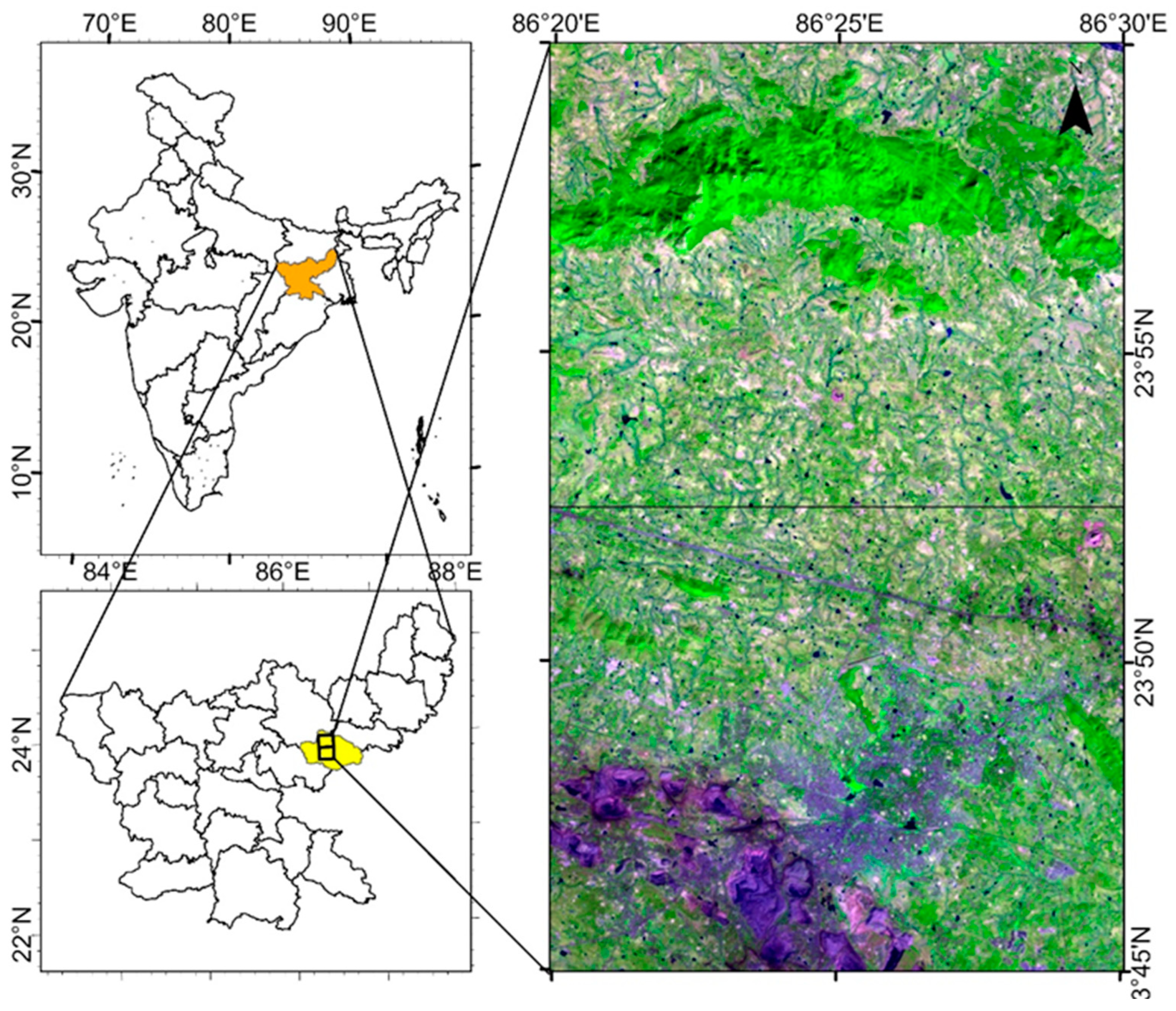
2. Description of Case Study Area
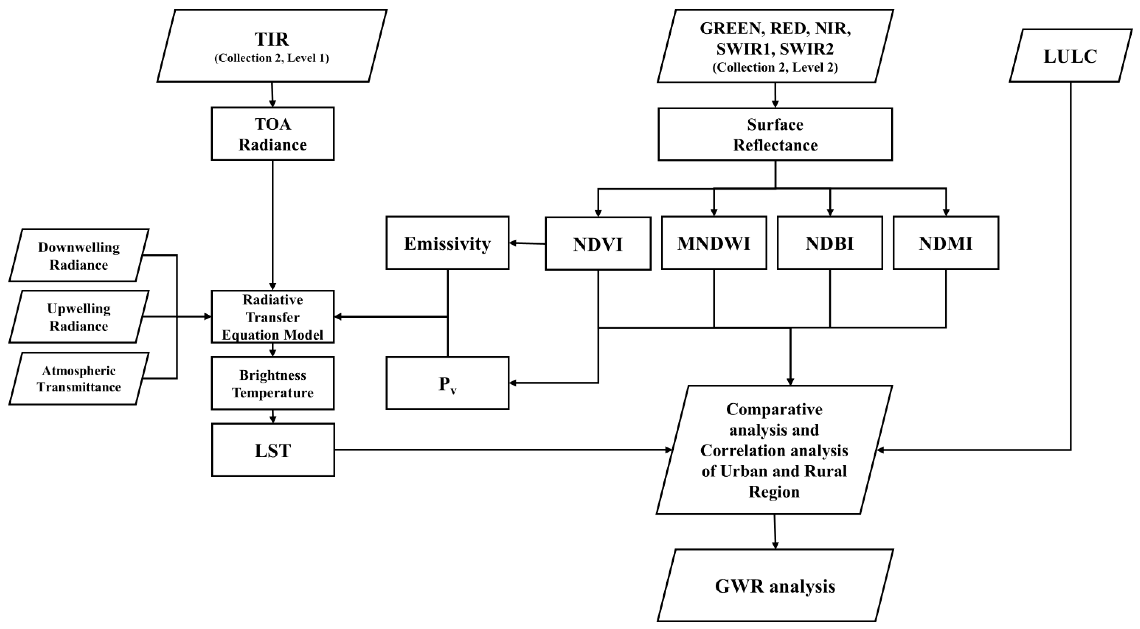
3. Data and Methodology
3.1. Conversion of Digital Number (DN) Values to Surface Reflectance
3.2. Land Use–Land Cover
3.3. Analysis Indices
3.3.1. Normalized Difference Vegetation Index (NDVI)
3.3.2. Modified Normalized Difference Water Index (MNDWI)
3.3.3. Normalized Difference Moisture Index (NDMI)
3.3.4. Normalized Difference Barren Index (NDBI)
3.4. Land Surface Temperature (LST)
3.5. Identification of Coal Fires
3.6. Geographically Weighted Regression (GWR)
4. Results and Discussions
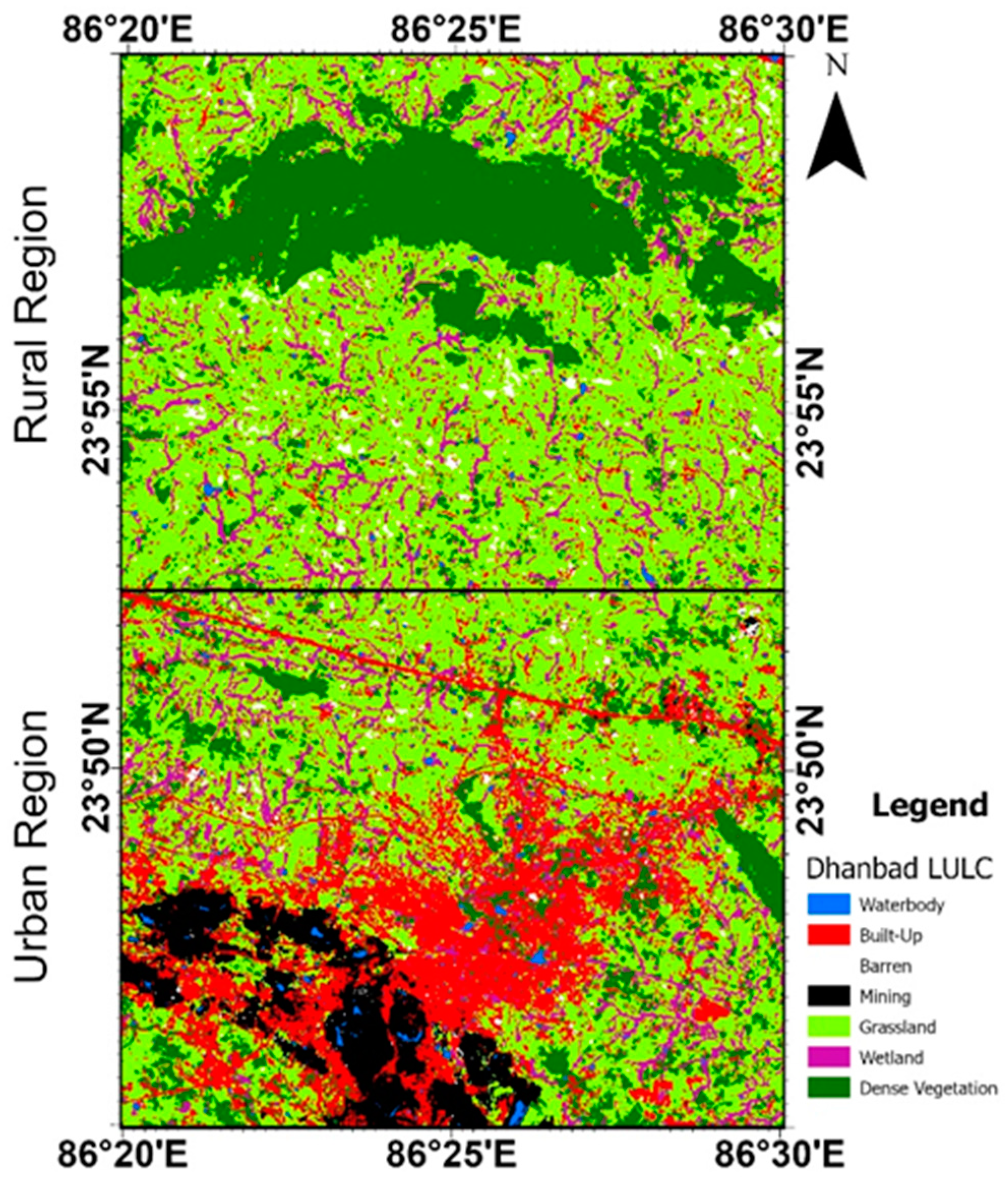
4.1. Land Use–Land Cover Map
4.2. NDVI Data
4.3. MNDWI Data
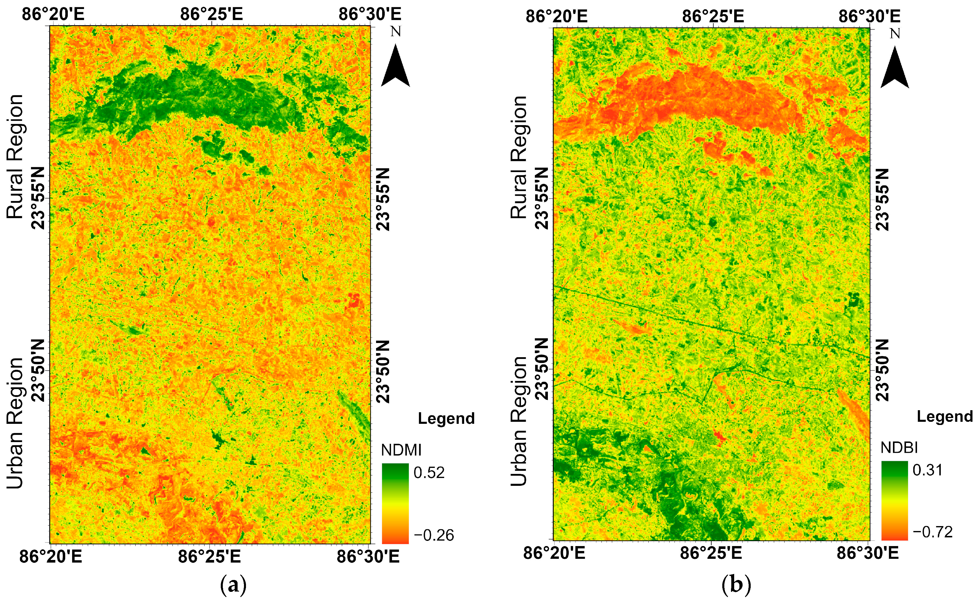
4.4. NDMI Data
4.5. NDBI Data
4.6. LST in Urban and Rural Areas
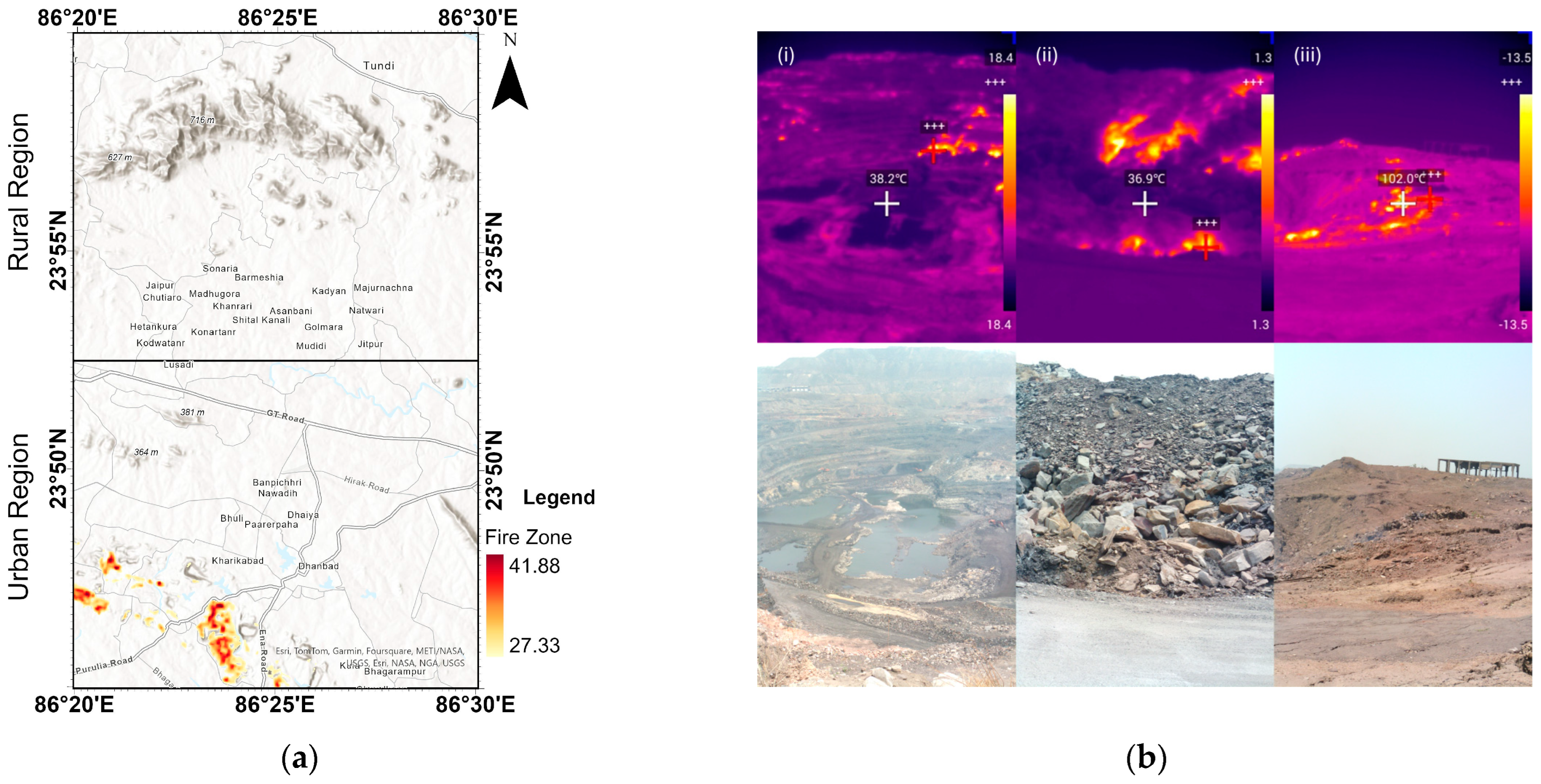
4.7. Identification of Coal Fire Areas
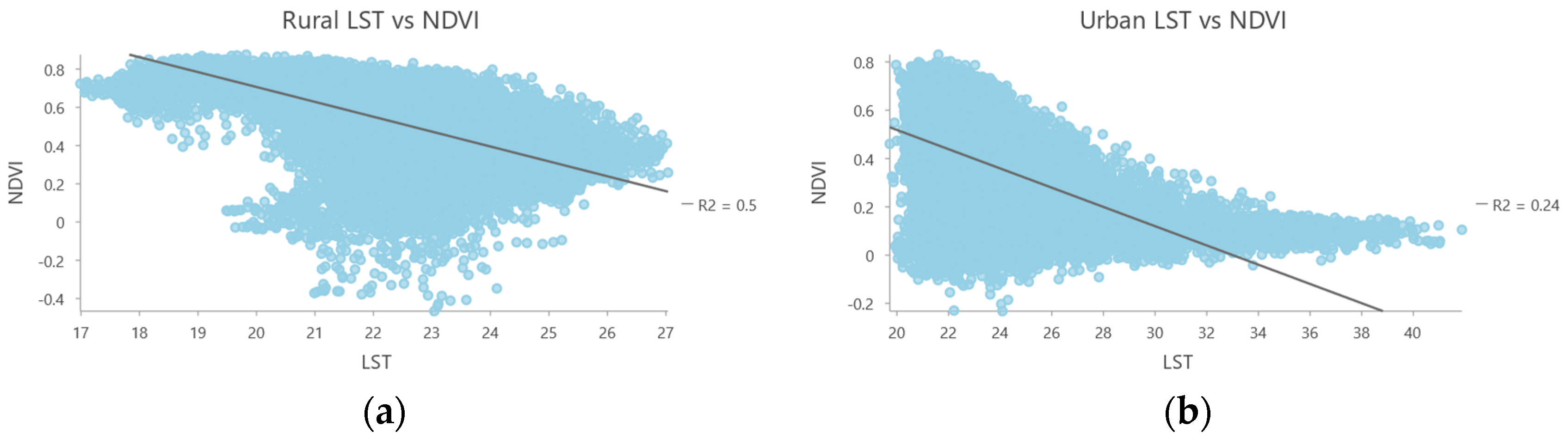
4.8. Relationship Between LST and Different Affecting Variables
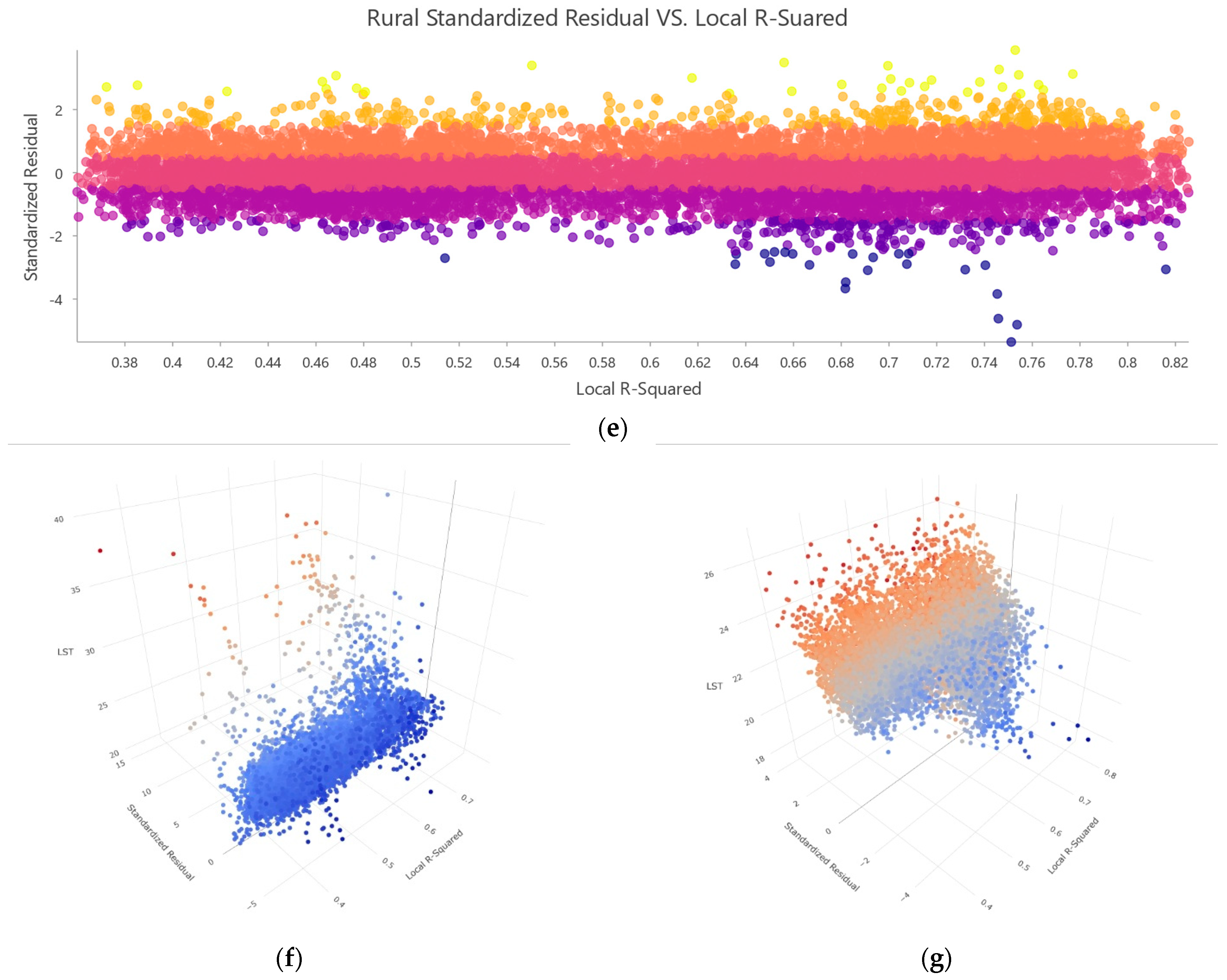
4.9. GWR Analysis
4.10. Limitations of the Study and Future Plans
5. Conclusions
Author Contributions
Funding
Data Availability Statement
Conflicts of Interest
References
- Zheng, Y.; Ren, C.; Xu, Y.; Wang, R.; Ho, J.; Lau, K.; Ng, E. GIS-Based Mapping of Local Climate Zone in the High-Density City of Hong Kong. Urban Clim. 2018, 24, 419–448. [Google Scholar] [CrossRef]
- Hu, J.; Yang, Y.; Pan, X.; Zhu, Q.; Zhan, W.; Wang, Y.; Ma, W.; Su, W. Analysis of the Spatial and Temporal Variations of Land Surface Temperature Based on Local Climate Zones: A Case Study in Nanjing, China. IEEE J. Sel. Top. Appl. Earth Obs. Remote Sens. 2019, 12, 4213–4223. [Google Scholar] [CrossRef]
- Ochola, E.M.; Fakharizadehshirazi, E.; Adimo, A.O.; Mukundi, J.B.; Wesonga, J.M.; Sodoudi, S. Inter-Local Climate Zone Differentiation of Land Surface Temperatures for Management of Urban Heat in Nairobi City, Kenya. Urban. Clim. 2020, 31, 100540. [Google Scholar] [CrossRef]
- International Energy Agency. Coal Mid-Year Update; International Energy Agency: Paris, France, 2024.
- Duda, A.; Valverde, G.F. The Economics of Coking Coal Mining: A Fossil Fuel Still Needed for Steel Production. Energies 2021, 14, 7682. [Google Scholar] [CrossRef]
- Phillips, J. Climate Change and Surface Mining: A Review of Environment-Human Interactions & Their Spatial Dynamics. Appl. Geogr. 2016, 74, 95–108. [Google Scholar]
- Oberschelp, C.; Pfister, S.; Raptis, C.E.; Hellweg, S. Global Emission Hotspots of Coal Power Generation. Nat. Sustain. 2019, 2, 113–121. [Google Scholar] [CrossRef]
- Ivanova, S.; Vesnina, A.; Fotina, N.; Prosekov, A. An Overview of Carbon Footprint of Coal Mining to Curtail Greenhouse Gas Emissions. Sustainability 2022, 14, 15135. [Google Scholar] [CrossRef]
- IPCC. Climate Change 2014: Synthesis Report; IPCC: Geneva, Switzerland, 2014.
- Onifade, M.; Genc, B. Spontaneous Combustion of Coals and Coal-Shales. Int. J. Min. Sci. Technol. 2018, 28, 933–940. [Google Scholar] [CrossRef]
- Bhagat, S.; Prasad, P.R.C. Assessing the Impact of Spatio-Temporal Land Use and Land Cover Changes on Land Surface Temperature, with a Major Emphasis on Mining Activities in the State of Chhattisgarh, India. Spat. Inf. Res. 2024, 32, 339–355. [Google Scholar] [CrossRef]
- Jaiswal, T.; Jhariya, D.; Kishore, N. The Effects of Coal Mining on Land Use and Land Surface Temperature: A Case Study of Korba District, Chhattisgarh. J. Environ. Inform. Lett. 2023, 10, 53–62. [Google Scholar] [CrossRef]
- Li, Q.; Guo, J.; Wang, F.; Song, Z. Monitoring the Characteristics of Ecological Cumulative Effect Due to Mining Disturbance Utilizing Remote Sensing. Remote Sens. 2021, 13, 5034. [Google Scholar] [CrossRef]
- Chaddad, F.; Mello, F.A.O.; Tayebi, M.; Safanelli, J.L.; Campos, L.R.; Amorim, M.T.A.; de Sousa, G.P.B.; Ferreira, T.O.; Ruiz, F.; Perlatti, F.; et al. Impact of Mining-Induced Deforestation on Soil Surface Temperature and Carbon Stocks: A Case Study Using Remote Sensing in the Amazon Rainforest. J. South. Am. Earth Sci. 2022, 119, 103983. [Google Scholar] [CrossRef]
- Siqi, J.; Yuhong, W. Effects of Land Use and Land Cover Pattern on Urban Temperature Variations: A Case Study in Hong Kong. Urban. Clim. 2020, 34, 100693. [Google Scholar] [CrossRef]
- Chatterjee, S.; Gupta, K. Urban Heat Island Formation in Relation to Land Transformation: A Study on a Mining Industrial Region of West Bengal. In Regional Development Planning and Practice: Contemporary Issues in South Asia; Mishra, M., Singh, R.B., Lucena, A.J., de Chatterjee, S., Eds.; Springer: Singapore, 2022; pp. 297–323. ISBN 978-981-16-5681-1. [Google Scholar]
- Cilek, M.U.; Cilek, A. Analyses of Land Surface Temperature (LST) Variability among Local Climate Zones (LCZs) Comparing Landsat-8 and ENVI-Met Model Data. Sustain. Cities Soc. 2021, 69, 102877. [Google Scholar] [CrossRef]
- Zhou, X.; Okaze, T.; Ren, C.; Cai, M.; Ishida, Y.; Watanabe, H.; Mochida, A. Evaluation of Urban Heat Islands Using Local Climate Zones and the Influence of Sea-Land Breeze. Sustain. Cities Soc. 2020, 55, 102060. [Google Scholar] [CrossRef]
- Sarker, T.; Fan, P.; Messina, J.P.; Macatangay, R.; Varnakovida, P.; Chen, J. Land Surface Temperature and Transboundary Air Pollution: A Case of Bangkok Metropolitan Region. Sci. Rep. 2024, 14, 10955. [Google Scholar] [CrossRef]
- Nimish, G.; Bharath, H.A.; Lalitha, A. Exploring Temperature Indices by Deriving Relationship Between Land Surface Temperature and Urban Landscape. Remote Sens. Appl. 2020, 18, 100299. [Google Scholar] [CrossRef]
- Taloor, A.K.; Manhas, D.S.; Kothyari, G.C. Retrieval of Land Surface Temperature, Normalized Difference Moisture Index, Normalized Difference Water Index of the Ravi Basin Using Landsat Data. Appl. Comput. Geosci. 2021, 9, 100051. [Google Scholar] [CrossRef]
- Xiang, Y.; Tang, Y.; Wang, Z.; Peng, C.; Huang, C.; Dian, Y.; Teng, M.; Zhou, Z. Seasonal Variations of the Relationship Between Spectral Indexes and Land Surface Temperature Based on Local Climate Zones: A Study in Three Yangtze River Megacities. Remote Sens. 2023, 15, 870. [Google Scholar] [CrossRef]
- Khalid, W.; Shamim, S.K.; Ahmad, A. Exploring Urban Land Surface Temperature with Geospatial and Regression Modelling Techniques in Uttarakhand Using SVM, OLS and GWR Models. Evol. Earth 2024, 2, 100038. [Google Scholar] [CrossRef]
- Xiao, X.D.; Dong, L.; Yan, H.; Yang, N.; Xiong, Y. The Influence of the Spatial Characteristics of Urban Green Space on the Urban Heat Island Effect in Suzhou Industrial Park. Sustain. Cities Soc. 2018, 40, 428–439. [Google Scholar] [CrossRef]
- Zhou, W.; Yu, W.; Zhang, Z.; Cao, W.; Wu, T. How Can Urban Green Spaces Be Planned to Mitigate Urban Heat Island Effect Under Different Climatic Backgrounds? A Threshold-Based Perspective. Sci. Total Environ. 2023, 890, 164422. [Google Scholar] [CrossRef] [PubMed]
- Yu, Z.; Guo, X.; Jørgensen, G.; Vejre, H. How Can Urban Green Spaces Be Planned for Climate Adaptation in Subtropical Cities? Ecol. Indic. 2017, 82, 152–162. [Google Scholar] [CrossRef]
- Masoudi, M.; Tan, P.Y. Multi-Year Comparison of the Effects of Spatial Pattern of Urban Green Spaces on Urban Land Surface Temperature. Landsc. Urban. Plan. 2019, 184, 44–58. [Google Scholar] [CrossRef]
- Zhou, W.; Wang, J.; Cadenasso, M.L. Effects of the Spatial Configuration of Trees on Urban Heat Mitigation: A Comparative Study. Remote Sens. Environ. 2017, 195, 1–12. [Google Scholar] [CrossRef]
- Hu, Z.; Xia, Q. An Integrated Methodology for Monitoring Spontaneous Combustion of Coal Waste Dumps Based on Surface Temperature Detection. Appl. Therm. Eng. 2017, 122, 27–38. [Google Scholar] [CrossRef]
- Cao, J.S.; Deng, Z.Y.; Li, W.; Hu, Y.D. Remote Sensing Inversion and Spatial Variation of Land Surface Temperature over Mining Areas of Jixi, Heilongjiang, China. PeerJ 2020, 8, e10257. [Google Scholar] [CrossRef]
- Mujawdiya, R.; Chatterjee, R.S.; Kumar, D. MODIS Land Surface Temperature Time Series Decomposition for Detecting and Characterizing Temporal Intensity Variations of Coal Fire Induced Thermal Anomalies in Jharia Coalfield, India. Geocarto Int. 2022, 37, 2160–2174. [Google Scholar] [CrossRef]
- Zhao, C.; Jensen, J.; Weng, Q.; Weaver, R. A Geographically Weighted Regression Analysis of the Underlying Factors Related to the Surface Urban Heat Island Phenomenon. Remote Sens. 2018, 10, 1428. [Google Scholar] [CrossRef]
- Guha, S.; Govil, H. Land Surface Temperature and Normalized Difference Vegetation Index Relationship: A Seasonal Study on a Tropical City. SN Appl. Sci. 2020, 2, 1661. [Google Scholar] [CrossRef]
- Ullah, W.; Ahmad, K.; Ullah, S.; Tahir, A.A.; Javed, M.F.; Nazir, A.; Abbasi, A.M.; Aziz, M.; Mohamed, A. Analysis of the Relationship among Land Surface Temperature (LST), Land Use Land Cover (LULC), and Normalized Difference Vegetation Index (NDVI) with Topographic Elements in the Lower Himalayan Region. Heliyon 2023, 9, e13322. [Google Scholar] [CrossRef]
- Ahmad, B.; Najar, M.B.; Ahmad, S. Analysis of LST, NDVI, and UHI Patterns for Urban Climate Using Landsat-9 Satellite Data in Delhi. J. Atmos. Sol. Terr. Phys. 2024, 265, 106359. [Google Scholar] [CrossRef]
- Yu, Z.; Xu, S.; Zhang, Y.; Jørgensen, G.; Vejre, H. Strong Contributions of Local Background Climate to the Cooling Effect of Urban Green Vegetation. Sci. Rep. 2018, 8, 6798. [Google Scholar] [CrossRef]
- Yucekaya, M.; Tirnakci, A. Microclimatic Effect of Urban Renewal: A Case Study of Kayseri/Turkey. Landsc. Ecol. Eng. 2023, 19, 471–483. [Google Scholar] [CrossRef]
- Manandhar, P.; Bande, L.; Tsoupos, A.; Marpu, P.R.; Armstrong, P. A Study of Local Climate Zones in Abu Dhabi with Urban Weather Stations and Numerical Simulations. Sustainability 2020, 12, 156. [Google Scholar] [CrossRef]
- Chi, Y.; Sun, J.; Sun, Y.; Liu, S.; Fu, Z. Multi-Temporal Characterization of Land Surface Temperature and Its Relationships with Normalized Difference Vegetation Index and Soil Moisture Content in the Yellow River Delta, China. Glob. Ecol. Conserv. 2020, 23, e01092. [Google Scholar] [CrossRef]
- Gao, Y.; Zhao, J.; Han, L. Exploring the Spatial Heterogeneity of Urban Heat Island Effect and Its Relationship to Block Morphology with the Geographically Weighted Regression Model. Sustain. Cities Soc. 2022, 76, 103431. [Google Scholar] [CrossRef]
- Yang, L.; Yu, K.; Ai, J.; Liu, Y.; Yang, W.; Liu, J. Dominant Factors and Spatial Heterogeneity of Land Surface Temperatures in Urban Areas: A Case Study in Fuzhou, China. Remote Sens. 2022, 14, 1266. [Google Scholar] [CrossRef]
- Jia, H.; Yang, D.; Deng, W.; Wei, Q.; Jiang, W. Predicting Land Surface Temperature with Geographically Weighed Regression and Deep Learning. Wiley Interdiscip. Rev. Data Min. Knowl. Discov. 2021, 11, e1396. [Google Scholar] [CrossRef]
- Li, H.; Xie, M.; Wang, H.; Li, S.; Xu, M. Spatial Heterogeneity of Vegetation Response to Mining Activities in Resource Regions of Northwestern China. Remote Sens. 2020, 12, 3247. [Google Scholar] [CrossRef]
- Kim, J.; Lin, S.Y.; Singh, R.P.; Lan, C.W.; Yun, H.W. Underground Burning of Jharia Coal Mine (India) and Associated Surface Deformation Using InSAR Data. Int. J. Appl. Earth Obs. Geoinf. 2021, 103, 102524. [Google Scholar] [CrossRef]
- Karanam, V.; Motagh, M.; Garg, S.; Jain, K. Multi-Sensor Remote Sensing Analysis of Coal Fire Induced Land Subsidence in Jharia Coalfields, Jharkhand, India. Int. J. Appl. Earth Obs. Geoinf. 2021, 102, 102439. [Google Scholar] [CrossRef]
- Singh, V.; Sardar, P.; Samadder, S.R.; Kumar, D.; Villuri, V.G.K. Predicting the Future Landscape of Dhanbad District: An Analysis of Land-Use Change and Urban Sprawl Through Cloud Computing and Neural Networks. Environ. Dev. Sustain. 2023, 26, 30749–30770. [Google Scholar] [CrossRef]
- IMD Pune. Climate of Jharkhand—Climatological Summaries of States Series—No. 17; IMD Pune: Pune, India, 2011.
- Fragou, S.; Kalogeropoulos, K.; Stathopoulos, N.; Louka, P.; Srivastava, P.K.; Karpouzas, S.; Kalivas, D.P.; Petropoulos, G.P. Quantifying Land Cover Changes in a Mediterranean Environment Using Lands at TM and Support Vector Machines. Forests 2020, 11, 750. [Google Scholar] [CrossRef]
- Huang, S.; Tang, L.; Hupy, J.P.; Wang, Y.; Shao, G. A Commentary Review on the Use of Normalized Difference Vegetation Index (NDVI) in the Era of Popular Remote Sensing. J. Res. 2021, 32, 1–6. [Google Scholar] [CrossRef]
- Tucker, C.J. Red and Photographic Infrared Linear Combinations for Monitoring Vegetation. Remote Sens. Environ. 1979, 8, 127–150. [Google Scholar]
- Xu, H. Modification of Normalised Difference Water Index (NDWI) to Enhance Open Water Features in Remotely Sensed Imagery. Int. J. Remote Sens. 2006, 27, 3025–3033. [Google Scholar] [CrossRef]
- Gao, B.-C. NDWI A Normalized Difference Water for Remote Sensing of Vegetation Water From Space. Remote Sens. Environ. 1996, 58, 257–266. [Google Scholar]
- Sekertekin, A.; Bonafoni, S. Land Surface Temperature Retrieval from Landsat 5, 7, and 8 over Rural Areas: Assessment of Different Retrieval Algorithms and Emissivity Models and Toolbox Implementation. Remote Sens. 2020, 12, 294. [Google Scholar] [CrossRef]
- Sobrino, J.A.; Jiménez-Muñoz, J.C.; Sòria, G.; Romaguera, M.; Guanter, L.; Moreno, J.; Plaza, A.; Martínez, P. Land Surface Emissivity Retrieval from Different VNIR and TIR Sensors. IEEE Trans. Geosci. Remote Sens. 2008, 46, 316–327. [Google Scholar]
- Carlson, T.N.; Riziley, D.A. On the Relation Between NDVI, Fractional Vegetation Cover, and Leaf Area Index. Remote Sens. Environ. 1997, 62, 241–252. [Google Scholar] [CrossRef]
- Biswal, S.S.; Gorai, A.K. Change Detection Analysis in Coverage Area of Coal Fire from 2009 to 2019 in Jharia Coalfield Using Remote Sensing Data. Int. J. Remote Sens. 2020, 41, 9545–9564. [Google Scholar] [CrossRef]
- Faka, A.; Kalogeropoulos, K.; Chalkias, C. Chapter 2—Quality of Life in Athens, Greece, Using Geonformatics. In Geoinformatics for Geosciences; Stathopoulos, N., Tsatsaris, A., Kalogeropoulos, K., Eds.; Earth Observation; Elsevier: Amsterdam, The Netherlands, 2023; pp. 31–44. ISBN 978-0-323-98983-1. [Google Scholar]
- Brunsdon, C.; Fotheringham, S.; Charlton, M. Geographically Weighted Regression. J. R. Stat. Soc. Ser. (Stat.) 1998, 47, 431–443. [Google Scholar] [CrossRef]
- Kawashima, S. Relation Between Vegetation, Surface Temperature, and Surface Composition Tokyo Region During Winter in The. Remote Sens. Environ. 1994, 50, 52–60. [Google Scholar] [CrossRef]
- Guha, S.; Govil, H.; Diwan, P. Analytical Study of Seasonal Variability in Land Surface Temperature with Normalized Difference Vegetation Index, Normalized Difference Water Index, Normalized Difference Built-Up Index, and Normalized Multiband Drought Index. J. Appl. Remote Sens. 2019, 13, 024518. [Google Scholar] [CrossRef]
- Guha, S.; Govil, H. Annual Assessment on the Relationship Between Land Surface Temperature and Six Remote Sensing Indices Using Landsat Data from 1988 to 2019. Geocarto Int. 2022, 37, 4292–4311. [Google Scholar] [CrossRef]
- Gupta, N.; Mathew, A.; Khandelwal, S. Analysis of Cooling Effect of Water Bodies on Land Surface Temperature in Nearby Region: A Case Study of Ahmedabad and Chandigarh Cities in India. Egypt. J. Remote Sens. Space Sci. 2019, 22, 81–93. [Google Scholar] [CrossRef]
- Hathway, E.A.; Sharples, S. The Interaction of Rivers and Urban Form in Mitigating the Urban Heat Island Effect: A UK Case Study. Build. Environ. 2012, 58, 14–22. [Google Scholar] [CrossRef]
- Onifade, M.; Genc, B. A Review of Research on Spontaneous Combustion of Coal. Int. J. Min. Sci. Technol. 2020, 30, 303–311. [Google Scholar] [CrossRef]
- Zheng, H.; Chen, Y.; Pan, W.; Cai, Y.; Chen, Z. Impact of Land Use/Land Cover Changes on the Thermal Environment in Urbanization: A Case Study of the Natural Wetlands Distribution Area in Minjiang River Estuary, China. Pol. J. Environ. Stud. 2019, 28, 3025–3041. [Google Scholar] [CrossRef]
- Taripanah, F.; Ranjbar, A. Quantitative Analysis of Spatial Distribution of Land Surface Temperature (LST) in Relation Ecohydrological, Terrain and Socio- Economic Factors Based on Landsat Data in Mountainous Area. Adv. Space Res. 2021, 68, 3622–3640. [Google Scholar] [CrossRef]
- Xu, Z.; Zhang, Z.; Li, C. Exploring Urban Green Spaces in China: Spatial Patterns, Driving Factors and Policy Implications. Land. Use Policy 2019, 89, 104249. [Google Scholar] [CrossRef]
- Zhang, M.; Yiğit, İ.; Adigüzel, F.; Hu, C.; Chen, E.; Siyavuş, A.E.; Elmastaş, N.; Ustuner, M.; Kaya, A.Y. Impact of Urban Surfaces on Microclimatic Conditions and Thermal Comfort in Burdur, Türkiye. Atmosphere 2024, 15, 1375. [Google Scholar] [CrossRef]
- Ge, X.; Mauree, D.; Castello, R.; Scartezzini, J.L. Spatio-Temporal Relationship between Land Cover and Land Surface Temperature in Urban Areas: A Case Study in Geneva and Paris. ISPRS Int. J. Geoinf. 2020, 9, 593. [Google Scholar] [CrossRef]
- Zhang, X.; Zhong, T.; Feng, X.; Wang, K. Estimation of the Relationship Between Vegetation Patches and Urban Land Surface Temperature with Remote Sensing. Int. J. Remote Sens. 2009, 30, 2105–2118. [Google Scholar] [CrossRef]
- Zhou, X.; Wang, Y.C. Dynamics of Land Surface Temperature in Response to Land-Use/Cover Change. Geogr. Res. 2011, 49, 23–36. [Google Scholar] [CrossRef]
- Chen, X.; Zhang, Y. Impacts of Urban Surface Characteristics on Spatiotemporal Pattern of Land Surface Temperature in Kunming of China. Sustain. Cities Soc. 2017, 32, 87–99. [Google Scholar] [CrossRef]
- Peng, J.; Jia, J.; Liu, Y.; Li, H.; Wu, J. Seasonal Contrast of the Dominant Factors for Spatial Distribution of Land Surface Temperature in Urban Areas. Remote Sens. Environ. 2018, 215, 255–267. [Google Scholar] [CrossRef]
- Lu, Y.; Feng, X.; Xiao, P.; Shen, C. Urban Heat Island in Summer of Nanjing Based on TM Data. In Proceedings of the 2009 Joint Urban Remote Sensing Event, Shanghai, China, 20–22 May 2009; p. 1. [Google Scholar]
- Siqi, J.; Yuhong, W.; Ling, C.; Xiaowen, B. A Novel Approach to Estimating Urban Land Surface Temperature by the Combination of Geographically Weighted Regression and Deep Neural Network Models. Urban. Clim. 2023, 47, 101390. [Google Scholar] [CrossRef]
- Oliveira, M.L.S.; da Boit, K.; Pacheco, F.; Teixeira, E.C.; Schneider, I.L.; Crissien, T.J.; Pinto, D.C.; Oyaga, R.M.; Silva, L.F.O. Multifaceted Processes Controlling the Distribution of Hazardous Compounds in the Spontaneous Combustion of Coal and the Effect of These Compounds on Human Health. Environ. Res. 2018, 160, 562–567. [Google Scholar] [CrossRef]
- Begum, N.; Maiti, A.; Chakravarty, D.; Das, B.S. Reflectance Spectroscopy Based Rapid Determination of Coal Quality Parameters. Fuel 2020, 280, 118676. [Google Scholar] [CrossRef]
- Peng, X.; Wu, W.; Zheng, Y.; Sun, J.; Hu, T.; Wang, P. Correlation Analysis of Land Surface Temperature and Topographic Elements in Hangzhou, China. Sci. Rep. 2020, 10, 10451. [Google Scholar] [CrossRef]


| Satellite | Sensor | Collection and Level | Year | Season, Date and Time * | Band Name | Wavelength (Micrometers) | Spatial Resolution (Meters) | |
|---|---|---|---|---|---|---|---|---|
| Summer | Winter | |||||||
| Landsat 8 | Operational Land Imager (OLI) | Collection 2, Level 2 | 2020 | 6 May 2020 10:12:22.68 | 15 January 2020 10:13:8.38 | Band 2—Blue | 0.452–0.512 | 30 |
| Band 3—Green | 0.533–0.590 | |||||||
| Band 4—Red | 0.636–0.673 | |||||||
| Band 5—Near-Infrared (NIR) | 0.851–0.879 | |||||||
| Band 6—Shortwave Infrared (SWIR) 1 | 1.566–1.651 | |||||||
| Band 7—Shortwave Infrared (SWIR) 2 | 2.107–2.294 | |||||||
| Landsat 8 | Thermal Infrared Sensor (TIRS) | Collection 2, Level 1 | 2020 | 6 May 2020 10:12:22.68 | 15 January 2020 10:13:8.38 | Band 10—Thermal Infrared (TIR) 1 | 10.600–11.190 | 100 (resampled to 30) |
| Range of Standardized Residuals | Category Name |
|---|---|
| <−2.5 | −C |
| −2.5 to −1.5 | −B |
| −1.5 to −0.5 | −A |
| −0.5 to 0.5 | A |
| 0.5 to 1.5 | +A |
| 1.5 to 2.5 | +B |
| >2.5 | +C |
| Rural LULC | NDVI | MNDWI | NDMI | NDBI | ||||||||||||
|---|---|---|---|---|---|---|---|---|---|---|---|---|---|---|---|---|
| Min | Max | Mean | Std | Min | Max | Mean | Std | Min | Max | Mean | Std | Min | Max | Mean | Std | |
| Waterbody | −0.31 | 0.56 | 0.17 | 0.17 | −0.34 | 0.67 | 0.13 | 0.22 | 0.01 | 0.48 | 0.25 | 0.09 | −0.64 | −0.20 | −0.44 | 0.10 |
| Built-up | 0.23 | 0.54 | 0.38 | 0.07 | −0.57 | −0.36 | −0.45 | 0.08 | −0.14 | 0.11 | −0.01 | 0.05 | −0.31 | 0.07 | −0.13 | 0.08 |
| Barren | 0.24 | 0.5 | 0.36 | 0.06 | −0.60 | −0.47 | −0.53 | 0.04 | −0.15 | −0.02 | −0.09 | 0.03 | −0.18 | 0.05 | −0.06 | 0.06 |
| Mining | 0.20 | 0.42 | 0.29 | 0.09 | −0.47 | −0.13 | −0.28 | 0.13 | −0.09 | 0.17 | 0.05 | 0.08 | −0.41 | −0.07 | −0.24 | 0.10 |
| Grassland | 0.33 | 0.68 | 0.51 | 0.06 | −0.60 | −0.43 | −0.51 | 0.03 | −0.11 | 0.20 | 0.03 | 0.05 | −0.47 | −0.02 | −0.25 | 0.08 |
| Wetland | 0.39 | 0.64 | 0.51 | 0.05 | −0.51 | −0.32 | −0.42 | 0.05 | 0.03 | 0.25 | 0.14 | 0.04 | −0.51 | −0.24 | −0.37 | 0.05 |
| Dense Vegetation | 0.55 | 0.84 | 0.73 | 0.06 | −0.57 | −0.43 | −0.5 | 0.03 | 0.05 | 0.43 | 0.25 | 0.06 | −0.72 | −0.28 | −0.53 | 0.08 |
| Urban LULC | NDVI | MNDWI | NDMI | NDBI | ||||||||||||
|---|---|---|---|---|---|---|---|---|---|---|---|---|---|---|---|---|
| Min | Max | Mean | Std | Min | Max | Mean | Std | Min | Max | Mean | Std | Min | Max | Mean | Std | |
| Waterbody | −0.14 | 0.57 | 0.19 | 0.15 | −0.33 | 0.56 | 0.06 | 0.19 | −0.06 | 0.52 | 0.19 | 0.11 | −0.70 | −0.08 | −0.35 | 0.15 |
| Built-up | 0.13 | 0.60 | 0.37 | 0.09 | −0.51 | −0.23 | −0.37 | 0.05 | −0.16 | 0.18 | 0.01 | 0.06 | −0.40 | 0.12 | −0.14 | 0.10 |
| Barren | 0.11 | 0.48 | 0.30 | 0.07 | −0.59 | −0.34 | −0.46 | 0.05 | −0.19 | −0.01 | −0.11 | 0.05 | −0.19 | 0.16 | 0.00 | 0.10 |
| Mining | 0.04 | 0.51 | 0.22 | 0.10 | −0.52 | −0.15 | −0.34 | 0.07 | −0.26 | 0.06 | −0.10 | 0.06 | −0.26 | 0.31 | 0.02 | 0.11 |
| Grassland | 0.34 | 0.69 | 0.52 | 0.06 | −0.57 | −0.38 | −0.48 | 0.04 | −0.1 | 0.21 | 0.05 | 0.06 | −0.48 | −0.06 | −0.27 | 0.08 |
| Wetland | 0.39 | 0.66 | 0.53 | 0.05 | −0.49 | −0.29 | −0.4 | 0.04 | 0.04 | 0.26 | 0.15 | 0.04 | −0.52 | −0.23 | −0.38 | 0.06 |
| Dense Vegetation | 0.51 | 0.79 | 0.65 | 0.06 | −0.56 | −0.33 | −0.44 | 0.05 | 0.06 | 0.33 | 0.19 | 0.05 | −0.64 | −0.27 | −0.46 | 0.07 |
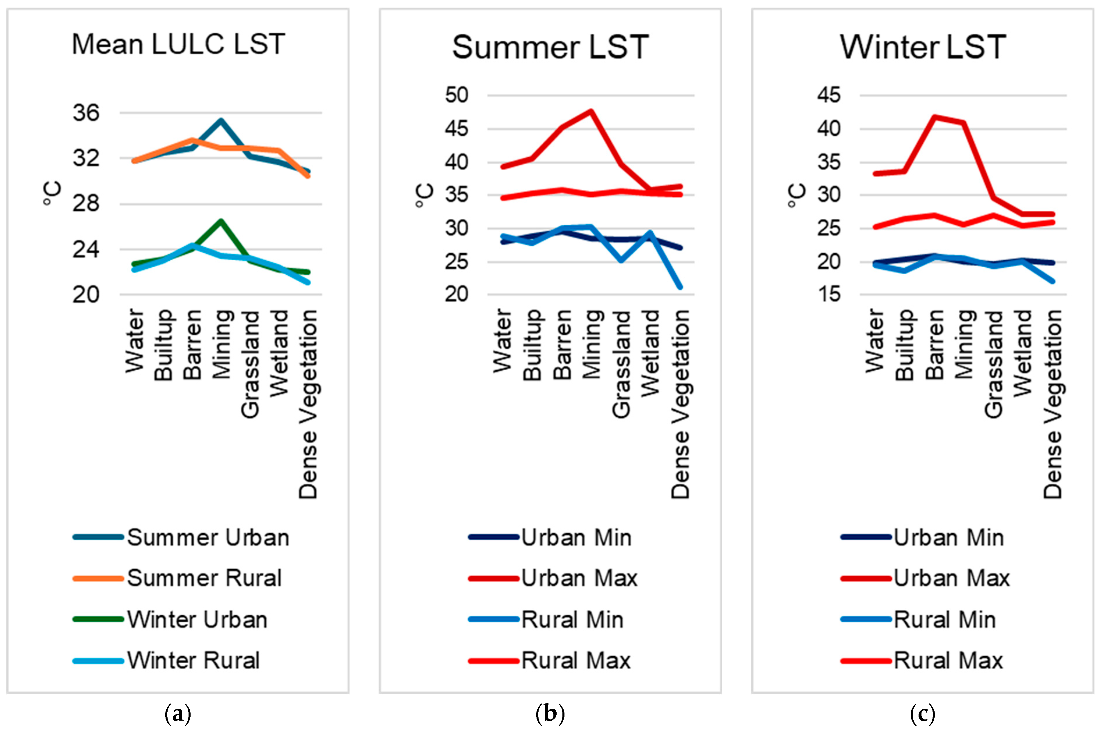
| Urban LST (°C) | Rural LST (°C) | ||||||||
|---|---|---|---|---|---|---|---|---|---|
| Season | LULC | Min | Max | Mean | Std | Min | Max | Mean | Std |
| Summer | Water | 28.03 | 39.32 | 31.74 | 1.87 | 28.77 | 34.66 | 31.8 | 1.05 |
| Built-up | 28.8 | 40.55 | 32.5 | 1.23 | 27.84 | 35.24 | 32.71 | 0.81 | |
| Barren | 29.62 | 45.3 | 32.95 | 1.35 | 30.09 | 35.77 | 33.58 | 0.7 | |
| Mining | 28.52 | 47.68 | 35.37 | 2.84 | 30.24 | 35.06 | 32.91 | 0.82 | |
| Grassland | 28.37 | 39.67 | 32.21 | 0.98 | 25.23 | 35.71 | 32.95 | 0.81 | |
| Wetland | 28.42 | 35.85 | 31.63 | 0.88 | 29.35 | 35.22 | 32.71 | 0.76 | |
| Dense Vegetation | 27.11 | 36.31 | 30.89 | 1.17 | 21.11 | 35.21 | 30.46 | 1.69 | |
| Winter | Water | 19.87 | 33.33 | 22.72 | 1.7 | 19.49 | 25.22 | 22.22 | 0.97 |
| Built-up | 20.31 | 33.64 | 23.08 | 1.18 | 18.56 | 26.39 | 23.02 | 0.86 | |
| Barren | 20.83 | 41.88 | 24.05 | 1.51 | 20.63 | 27.04 | 24.4 | 0.87 | |
| Mining | 20.02 | 41.01 | 26.47 | 3.33 | 20.55 | 25.58 | 23.44 | 0.9 | |
| Grassland | 19.72 | 29.57 | 22.99 | 0.81 | 19.36 | 27.02 | 23.2 | 0.84 | |
| Wetland | 20.1 | 27.11 | 22.19 | 0.58 | 20.03 | 25.41 | 22.45 | 0.62 | |
| Dense Vegetation | 19.81 | 27.1 | 21.99 | 0.66 | 16.99 | 25.86 | 21.09 | 1.18 | |
Disclaimer/Publisher’s Note: The statements, opinions and data contained in all publications are solely those of the individual author(s) and contributor(s) and not of MDPI and/or the editor(s). MDPI and/or the editor(s) disclaim responsibility for any injury to people or property resulting from any ideas, methods, instructions or products referred to in the content. |
© 2025 by the authors. Licensee MDPI, Basel, Switzerland. This article is an open access article distributed under the terms and conditions of the Creative Commons Attribution (CC BY) license (https://creativecommons.org/licenses/by/4.0/).
Share and Cite
Kandulna, W.; Jain, M.K.; Chugh, Y.P.; Agarwal, S. Spatial Variability of Land Surface Temperature of a Coal Mining Region Using a Geographically Weighted Regression Model: A Case Study. Land 2025, 14, 696. https://doi.org/10.3390/land14040696
Kandulna W, Jain MK, Chugh YP, Agarwal S. Spatial Variability of Land Surface Temperature of a Coal Mining Region Using a Geographically Weighted Regression Model: A Case Study. Land. 2025; 14(4):696. https://doi.org/10.3390/land14040696
Chicago/Turabian StyleKandulna, Wilson, Manish Kumar Jain, Yoginder P. Chugh, and Siddhartha Agarwal. 2025. "Spatial Variability of Land Surface Temperature of a Coal Mining Region Using a Geographically Weighted Regression Model: A Case Study" Land 14, no. 4: 696. https://doi.org/10.3390/land14040696
APA StyleKandulna, W., Jain, M. K., Chugh, Y. P., & Agarwal, S. (2025). Spatial Variability of Land Surface Temperature of a Coal Mining Region Using a Geographically Weighted Regression Model: A Case Study. Land, 14(4), 696. https://doi.org/10.3390/land14040696