


Exploration of Spatiotemporal Covariation in Vegetation–Groundwater Relationships: A Case Study in an Endorheic Inland River Basin


Abstract
1. Introduction
2. Materials and Methods
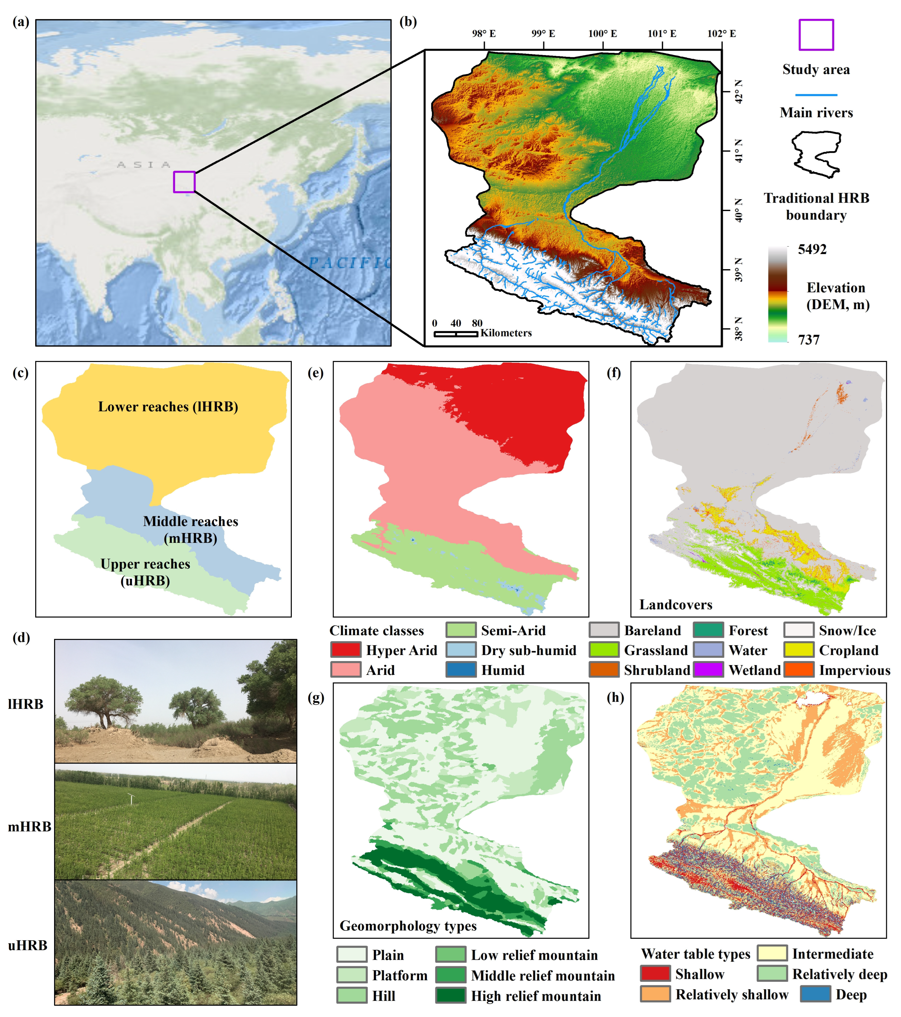
2.1. Study Area
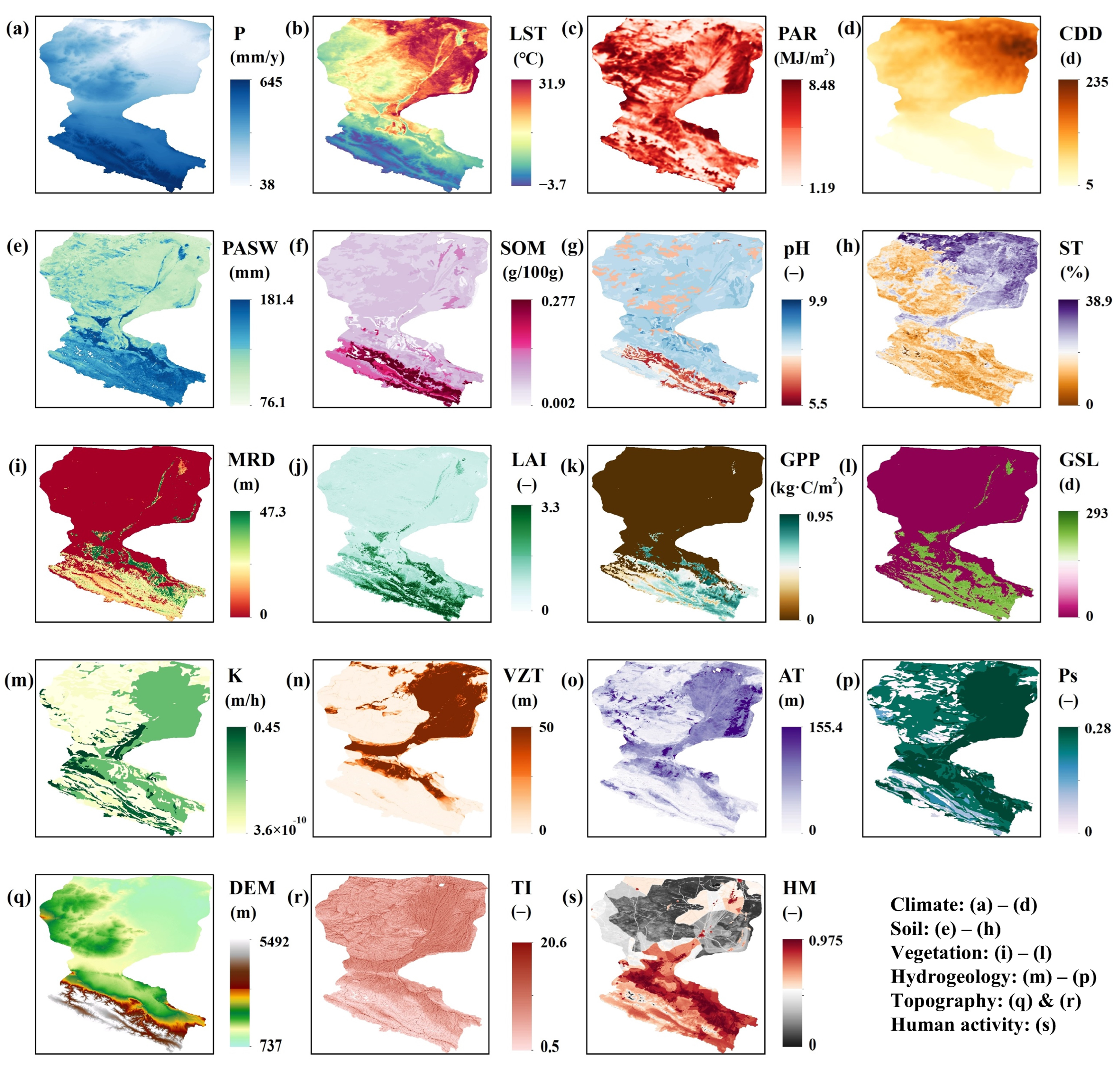
2.2. Dataset

| Parameter/Variable | Acronym | Original Spatial | Original Temporal | Source | ||
|---|---|---|---|---|---|---|
| Domain | Resolution | Period | Resolution | |||
| Climate class | - | Global | 30 arc-second | 1960–2000 | - | [75] |
| Landcover type | - | Qilian Mountain Area | 30 m | 1990–2020 | 5-year | [76] |
| Geomorphology type | - | China | 1 km | - | - | - |
| Water table depth | WTD | Global | 30 arc-second | 2003–2013 | Monthly | [41] |
| Normalized difference vegetation index | NDVI | HRB | 0.01 degree | 2001–2011 | Daily | [74] |
| Precipitation | P | China | 0.025 degree | 1951–2011 | Monthly | [77] |
| Land surface temperature | LST | China | 1 km | 2000–2022 | Daily | [78] |
| Photosynthetic effective radiation | PAR | HRB | 1 km | 2010–2015 | Hourly | [79] |
| Consecutive dry days | CDD | Global | 0.1 degree | - | - | [80] |
| Plant-available soil water | PASW | Global | 0.5 degree | - | - | [81] |
| Soil organic matter | SOM | China | 30 arc-second | - | - | [82] |
| Soil pondus hydrogenii | pH | China | 30 arc-second | - | - | [82] |
| Soil texture | ST | Global | 30 arc-second | - | - | [83] |
| Maximum rooting depth | MRD | Global | 30 arc-second | 2003–2013 | Monthly | [84] |
| Leaf area index | LA | HRB | 30 m | 2011–2015 | Monthly | [85] |
| Gross primary productivity | GPP | Global | 1 km | 2001–2023 | Monthly | - |
| Growing season length | GSL | Global | 300 m | - | - | [86] |
| Porosity | Ps | Global | Vector | - | - | [87] |
| Saturated hydraulic conductivity | Ks | Global | Vector | - | - | [87] |
| Aquifer thickness | AT | Global | 3 arc-second | - | - | [88] |
| Vadose zone thickness | VZT | Global | 30 arc-second | - | - | [89] |
| Digital elevation model | DEM | Qilian Mountain area | 30 m | 2018 | - | [90] |
| Topographic index | TI | Global | 30 arc-second | - | - | [91] |
| Human modification | HM | Global | 30 arc-second | 2016 1 | - | [92] |
| Groundwater-dependent ecosystem | GDE | Global | 30 m | - | - | [93] |
2.3. Methods
2.3.1. Spearman’s Rank Correlation Analysis
2.3.2. Cross-Correlation Analysis
2.3.3. Generalized Additive Model (GAM)
3. Results
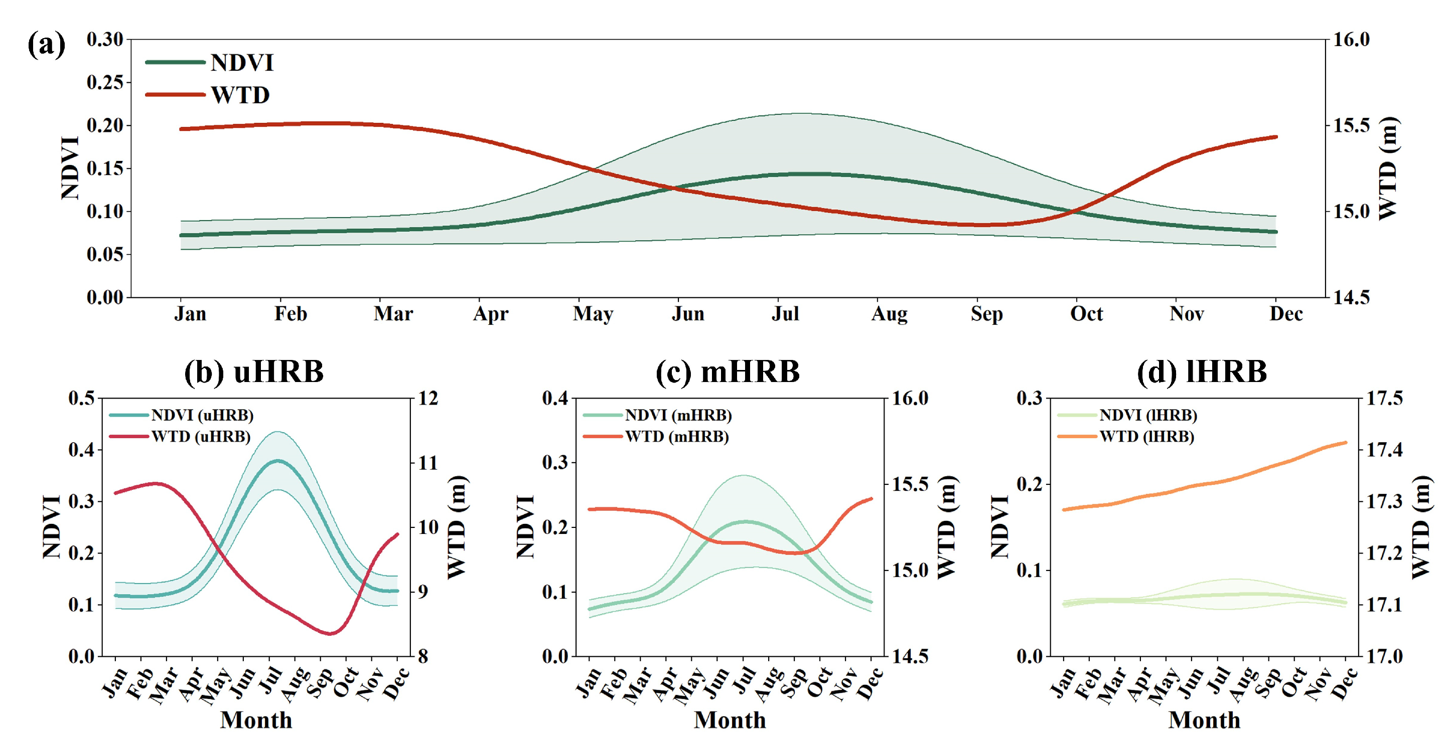
3.1. Seasonal Dynamics of Vegetation–Groundwater Relationships
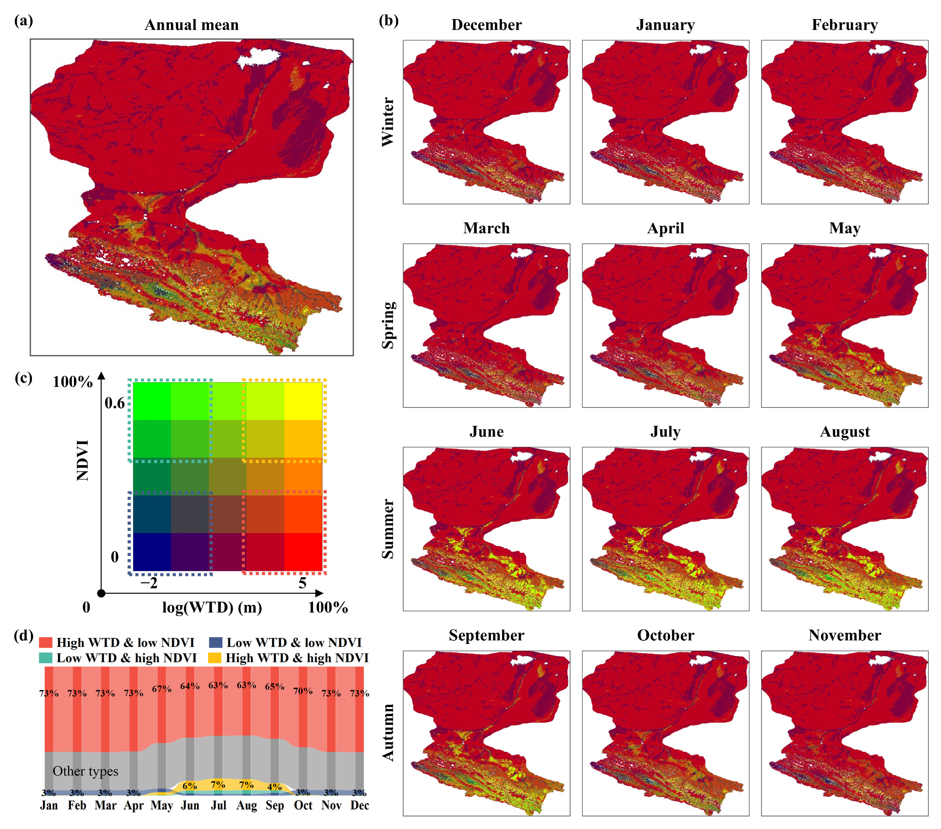
3.2. Spatiotemporal Distribution of Vegetation–Groundwater Relationships
3.3. Variability in the NDVI–WTD Correlations Across Landcover Types and Climate Zones
3.4. Variability in the NDVI–WTD Correlations with Geomorphological Characteristics
3.5. Association with Groundwater-Dependent Ecosystems (GDE) Area
3.6. Contributions of Environmental Variables
4. Discussion
4.1. Application of the NDVI–WTD Relationships in Investigating Vegetation-Groundwater Interactions
4.2. Utilization of Generalized Additive Models (GAMs) in Vegetation-Groundwater Studies
4.3. Factors Influencing the Contributions of Environmental Variables
5. Conclusions
Supplementary Materials
Author Contributions
Funding
Data Availability Statement
Acknowledgments
Conflicts of Interest
References
- Scanlon, B.R.; Fakhreddine, S.; Rateb, A.; De Graaf, I.; Famiglietti, J.; Gleeson, T.; Grafton, R.Q.; Jobbagy, E.; Kebede, S.; Kolusu, S.R.; et al. Global Water Resources and the Role of Groundwater in a Resilient Water Future. Nat. Rev. Earth Environ. 2023, 4, 87–101. [Google Scholar] [CrossRef]
- Thornton, J.M. Mountain Streamflow Threatened by Irreversible Simulated Groundwater Declines. Nat. Water 2024, 2, 403–404. [Google Scholar] [CrossRef]
- Gleeson, T.; Cuthbert, M.; Ferguson, G.; Perrone, D. Global Groundwater Sustainability, Resources, and Systems in the Anthropocene. Annu. Rev. Earth Planet. Sci. 2020, 48, 431–463. [Google Scholar]
- Liu, X.; Wang, N.; Wang, Y.; Meng, N.; Wang, Y.; Qiao, B.; Lu, R.; Yang, D. Research on Groundwater Drought and Sustainability in Badain Jaran Desert and Surrounding Areas Based on GRACE Satellite. Land 2025, 14, 173. [Google Scholar] [CrossRef]
- Maxwell, R.M.; Condon, L.E. Connections between Groundwater Flow and Transpiration Partitioning. Science 2016, 353, 377–380. [Google Scholar] [CrossRef]
- Gentine, P.; Green, J.K.; Guérin, M.; Humphrey, V.; Seneviratne, S.I.; Zhang, Y.; Zhou, S. Coupling between the Terrestrial Carbon and Water Cycles—A Review. Environ. Res. Lett. 2019, 14, 083003. [Google Scholar] [CrossRef]
- Koirala, S.; Jung, M.; Reichstein, M.; De Graaf, I.E.M.; Camps-Valls, G.; Ichii, K.; Papale, D.; Ráduly, B.; Schwalm, C.R.; Tramontana, G.; et al. Global Distribution of Groundwater-vegetation Spatial Covariation. Geophys. Res. Lett. 2017, 44, 4134–4142. [Google Scholar] [CrossRef]
- Jiao, W.; Wang, L.; Smith, W.K.; Chang, Q.; Wang, H.; D’Odorico, P. Observed Increasing Water Constraint on Vegetation Growth over the Last Three Decades. Nat. Commun. 2021, 12, 3777. [Google Scholar] [CrossRef]
- Glanville, K.; Sheldon, F.; Butler, D.; Capon, S. Effects and Significance of Groundwater for Vegetation: A Systematic Review. Sci. Total Environ. 2023, 875, 162577. [Google Scholar] [CrossRef]
- Bernardino, P.N.; De Keersmaecker, W.; Horion, S.; Oehmcke, S.; Gieseke, F.; Fensholt, R.; Van De Kerchove, R.; Lhermitte, S.; Abel, C.; Van Meerbeek, K.; et al. Predictability of Abrupt Shifts in Dryland Ecosystem Functioning. Nat. Clim. Chang. 2025, 15, 86–91. [Google Scholar] [CrossRef]
- Huggins, X.; Gleeson, T.; Serrano, D.; Zipper, S.; Jehn, F.; Rohde, M.M.; Abell, R.; Vigerstol, K.; Hartmann, A. Overlooked Risks and Opportunities in Groundwatersheds of the World’s Protected Areas. Nat. Sustain. 2023, 6, 855–864. [Google Scholar] [CrossRef]
- Rohde, M.M.; Stella, J.C.; Singer, M.B.; Roberts, D.A.; Caylor, K.K.; Albano, C.M. Establishing Ecological Thresholds and Targets for Groundwater Management. Nat. Water 2024, 2, 312–323. [Google Scholar] [CrossRef]
- Huggins, X.; Gleeson, T.; Villholth, K.G.; Rocha, J.C.; Famiglietti, J.S. Groundwaterscapes: A Global Classification and Mapping of Groundwater’s Large-Scale Socioeconomic, Ecological, and Earth System Functions. Water Resour. Res. 2024, 60, e2023WR036287. [Google Scholar] [CrossRef]
- Link, A.; El-Hokayem, L.; Usman, M.; Conrad, C.; Reinecke, R.; Berger, M.; Wada, Y.; Coroama, V.; Finkbeiner, M. Groundwater-Dependent Ecosystems at Risk—Global Hotspot Analysis and Implications. Environ. Res. Lett. 2023, 18, 094026. [Google Scholar] [CrossRef]
- Perrone, D.; Rohde, M.M.; Hammond Wagner, C.; Anderson, R.; Arthur, S.; Atume, N.; Brown, M.; Esaki-Kua, L.; Gonzalez Fernandez, M.; Garvey, K.A.; et al. Stakeholder Integration Predicts Better Outcomes from Groundwater Sustainability Policy. Nat. Commun. 2023, 14, 3793. [Google Scholar] [CrossRef] [PubMed]
- Chan, F.K.S.; Paszkowski, A.; Wang, Z.; Lu, X.; Mitchell, G.; Tran, D.D.; Warner, J.; Li, J.; Chen, Y.D.; Li, N.; et al. Building Resilience in Asian Mega-Deltas. Nat. Rev. Earth Environ. 2024, 5, 522–537. [Google Scholar] [CrossRef]
- Gleeson, T.; Alley, W.M.; Allen, D.M.; Sophocleous, M.A.; Zhou, Y.; Taniguchi, M.; VanderSteen, J. Towards Sustainable Groundwater Use: Setting Long-Term Goals, Backcasting, and Managing Adaptively. Groundwater 2012, 50, 19–26. [Google Scholar] [CrossRef]
- Lu, Z.; He, Y.; Peng, S. Assessing Integrated Hydrologic Model: From Benchmarking to Case Study in a Typical Arid and Semi-Arid Basin. Land 2023, 12, 697. [Google Scholar] [CrossRef]
- Scanlon, B.R.; Keese, K.E.; Flint, A.L.; Flint, L.E.; Gaye, C.B.; Edmunds, W.M.; Simmers, I. Global Synthesis of Groundwater Recharge in Semiarid and Arid Regions. Hydrol. Process. 2006, 20, 3335–3370. [Google Scholar] [CrossRef]
- Zeng, Y.; Xie, Z.; Yu, Y.; Liu, S.; Wang, L.; Jia, B.; Qin, P.; Chen, Y. Ecohydrological Effects of Stream–Aquifer Water Interaction: A Case Study of the Heihe River Basin, Northwestern China. Hydrol. Earth Syst. Sci. 2016, 20, 2333–2352. [Google Scholar] [CrossRef]
- Yao, Y.; Zheng, C.; Tian, Y.; Li, X.; Liu, J. Eco-hydrological Effects Associated with Environmental Flow Management: A Case Study from the Arid Desert Region of China. Ecohydrology 2018, 11, e1914. [Google Scholar] [CrossRef]
- Wang, T.; Wu, Z.; Wang, P.; Wu, T.; Zhang, Y.; Yin, J.; Yu, J.; Wang, H.; Guan, X.; Xu, H.; et al. Plant-Groundwater Interactions in Drylands: A Review of Current Research and Future Perspectives. Agric. For. Meteorol. 2023, 341, 109636. [Google Scholar] [CrossRef]
- Bernardino, P.N.; De Keersmaecker, W.; Fensholt, R.; Verbesselt, J.; Somers, B.; Horion, S. Global-scale Characterization of Turning Points in Arid and Semi-arid Ecosystem Functioning. Global Ecol. Biogeogr. 2020, 29, 1230–1245. [Google Scholar] [CrossRef]
- O’Connor, J.; Santos, M.J.; Rebel, K.T.; Dekker, S.C. The Influence of Water Table Depth on Evapotranspiration in the Amazon Arc of Deforestation. Hydrol. Earth Syst. Sci. 2019, 23, 3917–3931. [Google Scholar] [CrossRef]
- Zhao, T.; Zhu, Y.; Ye, M.; Yang, J.; Jia, B.; Mao, W.; Wu, J. A New Approach for Estimating Spatial-Temporal Phreatic Evapotranspiration at a Regional Scale Using NDVI and Water Table Depth Measurements. Agric. Water Manag. 2022, 264, 107500. [Google Scholar] [CrossRef]
- Šimanauskienė, R.; Linkevičienė, R.; Bartold, M.; Dąbrowska-Zielińska, K.; Slavinskienė, G.; Veteikis, D.; Taminskas, J. Peatland Degradation: The Relationship between Raised Bog Hydrology and Normalized Difference Vegetation Index. Ecohydrology 2019, 12, e2159. [Google Scholar] [CrossRef]
- Eamus, D.; Zolfaghar, S.; Villalobos-Vega, R.; Cleverly, J.; Huete, A. Groundwater-Dependent Ecosystems: Recent Insights from Satellite and Field-Based Studies. Hydrol. Earth Syst. Sci. 2015, 19, 4229–4256. [Google Scholar] [CrossRef]
- Bierkens, M.F.P.; Wada, Y. Non-Renewable Groundwater Use and Groundwater Depletion: A Review. Environ. Res. Lett. 2019, 14, 063002. [Google Scholar] [CrossRef]
- Li, W.; Manzanedo, R.D.; Jiang, Y.; Ma, W.; Du, E.; Zhao, S.; Rademacher, T.; Dong, M.; Xu, H.; Kang, X.; et al. Reassessment of Growth-Climate Relations Indicates the Potential for Decline across Eurasian Boreal Larch Forests. Nat. Commun. 2023, 14, 3358. [Google Scholar] [CrossRef]
- Sutanto, S.J.; Syaehuddin, W.A.; De Graaf, I. Hydrological Drought Forecasts Using Precipitation Data Depend on Catchment Properties and Human Activities. Commun. Earth Environ. 2024, 5, 118. [Google Scholar] [CrossRef]
- Koppa, A.; Keune, J.; Schumacher, D.L.; Michaelides, K.; Singer, M.; Seneviratne, S.I.; Miralles, D.G. Dryland Self-Expansion Enabled by Land–Atmosphere Feedbacks. Science 2024, 385, 967–972. [Google Scholar] [CrossRef]
- Rambhunjun, P.; Bertone, F.; Rossignol, A.; Sou, M. Mapping Sahelian Groundwater-Dependent Ecosystems Based on an Updated Typology. Hydrogeol. J. 2024, 32, 2031–2049. [Google Scholar] [CrossRef]
- Xu, W.; Kong, F.; Mao, R.; Song, J.; Sun, H.; Wu, Q.; Liang, D.; Bai, H. Identifying and Mapping Potential Groundwater-Dependent Ecosystems for a Semi-Arid and Semi-Humid Area in the Weihe River, China. J. Hydrol. 2022, 609, 127789. [Google Scholar] [CrossRef]
- Fildes, S.G.; Doody, T.M.; Bruce, D.; Clark, I.F.; Batelaan, O. Mapping Groundwater Dependent Ecosystem Potential in a Semi-Arid Environment Using a Remote Sensing-Based Multiple-Lines-of-Evidence Approach. Int. J. Digit. Earth 2023, 16, 375–406. [Google Scholar] [CrossRef]
- Duran-Llacer, I.; Arumí, J.L.; Arriagada, L.; Aguayo, M.; Rojas, O.; González-Rodríguez, L.; Rodríguez-López, L.; Martínez-Retureta, R.; Oyarzún, R.; Singh, S.K. A New Method to Map Groundwater-Dependent Ecosystem Zones in Semi-Arid Environments: A Case Study in Chile. Sci. Total Environ. 2022, 816, 151528. [Google Scholar] [CrossRef]
- Reinecke, R.; Gnann, S.; Stein, L.; Bierkens, M.; De Graaf, I.; Gleeson, T.; Essink, G.O.; Sutanudjaja, E.H.; Ruz Vargas, C.; Verkaik, J.; et al. Uncertainty in Model Estimates of Global Groundwater Depth. Environ. Res. Lett. 2024, 19, 114066. [Google Scholar] [CrossRef]
- Taylor, R.G.; Scanlon, B.; Döll, P.; Rodell, M.; Van Beek, R.; Wada, Y.; Longuevergne, L.; Leblanc, M.; Famiglietti, J.S.; Edmunds, M.; et al. Ground Water and Climate Change. Nature Clim. Chang. 2013, 3, 322–329. [Google Scholar] [CrossRef]
- Curran, D.; Gleeson, T.; Huggins, X. Applying a Science-Forward Approach to Groundwater Regulatory Design. Hydrogeol. J. 2023, 31, 853–871. [Google Scholar] [CrossRef]
- Huggins, X.; Gleeson, T.; Castilla-Rho, J.; Holley, C.; Re, V.; Famiglietti, J.S. Groundwater Connections and Sustainability in Social-Ecological Systems. Groundwater 2023, 61, 463–478. [Google Scholar] [CrossRef]
- Saito, L.; Christian, B.; Diffley, J.; Richter, H.; Rohde, M.M.; Morrison, S.A. Managing Groundwater to Ensure Ecosystem Function. Groundwater 2021, 59, 322–333. [Google Scholar] [CrossRef]
- Fan, Y.; Li, H.; Miguez-Macho, G. Global Patterns of Groundwater Table Depth. Science 2013, 339, 940–943. [Google Scholar] [CrossRef] [PubMed]
- D’Acunha, B.; Lee, S.; Johnson, M.S. Ecohydrological Responses to Rewetting of a Highly Impacted Raised Bog Ecosystem. Ecohydrology 2018, 11, e1922. [Google Scholar] [CrossRef]
- Fan, Y.; Miguez-Macho, G. Infiltration Depth, Rooting Depth, and Regolith Flushing—A Global Perspective. PNAS Nexus 2024, 3, pgae514. [Google Scholar] [CrossRef]
- Miguez-Macho, G.; Fan, Y. Spatiotemporal Origin of Soil Water Taken up by Vegetation. Nature 2021, 598, 624–628. [Google Scholar] [CrossRef] [PubMed]
- Griebler, C.; Avramov, M. Groundwater Ecosystem Services: A Review. Freshw. Sci. 2015, 34, 355–367. [Google Scholar] [CrossRef]
- Hou, X.; Yang, H.; Cao, J.; Feng, W.; Zhang, Y. A Review of Advances in Groundwater Evapotranspiration Research. Water 2023, 15, 969. [Google Scholar] [CrossRef]
- Li, M.; Li, F.; Fu, S.; Chen, H.; Wang, K.; Chen, X.; Huang, J. Identification, Mapping, and Eco-Hydrological Signal Analysis for Groundwater-Dependent Ecosystems (GDEs) in Langxi River Basin, North China. Hydrol. Earth Syst. Sci. 2024, 28, 4623–4642. [Google Scholar] [CrossRef]
- MacAllister, D.J.; Krishan, G.; Basharat, M.; Cuba, D.; MacDonald, A.M. A Century of Groundwater Accumulation in Pakistan and Northwest India. Nat. Geosci. 2022, 15, 390–396. [Google Scholar] [CrossRef]
- An, Q.; Staal, A.; Liu, L.; Cheng, Y.; Liu, J.; Huang, G. Crops Feed Rain to Drylands in Northwest China. Earth’s Future 2024, 12, e2024EF004791. [Google Scholar] [CrossRef]
- Lian, X.; Piao, S.; Chen, A.; Huntingford, C.; Fu, B.; Li, L.Z.X.; Huang, J.; Sheffield, J.; Berg, A.M.; Keenan, T.F.; et al. Multifaceted Characteristics of Dryland Aridity Changes in a Warming World. Nat. Rev. Earth Environ. 2021, 2, 232–250. [Google Scholar] [CrossRef]
- Rohde, M.M.; Stella, J.C.; Roberts, D.A.; Singer, M.B. Groundwater Dependence of Riparian Woodlands and the Disrupting Effect of Anthropogenically Altered Streamflow. Proc. Natl. Acad. Sci. USA 2021, 118, e2026453118. [Google Scholar] [CrossRef] [PubMed]
- Elshall, A.S.; Arik, A.D.; El-Kadi, A.I.; Pierce, S.; Ye, M.; Burnett, K.M.; Wada, C.A.; Bremer, L.L.; Chun, G. Groundwater Sustainability: A Review of the Interactions between Science and Policy. Environ. Res. Lett. 2020, 15, 93004. [Google Scholar] [CrossRef]
- Shen, X.; Niu, L.; Jia, X.; Yang, T.; Hu, W.; Wu, C.; Chu, J.; Biswas, A.; Shao, M. Disentangling Ecological Restoration’s Impact on Terrestrial Water Storage. Geophys. Res. Lett. 2025, 52, e2024GL111669. [Google Scholar] [CrossRef]
- Rodell, M.; Reager, J.T. Water Cycle Science Enabled by the GRACE and GRACE-FO Satellite Missions. Nat. Water 2023, 1, 47–59. [Google Scholar] [CrossRef]
- Lu, Z.; Wei, J.; Yang, X. Effects of Hydraulic Conductivity on Simulating Groundwater–Land Surface Interactions over a Typical Endorheic River Basin. J. Hydrol. 2024, 638, 131542. [Google Scholar] [CrossRef]
- Cai, L.; Kreft, H.; Taylor, A.; Denelle, P.; Schrader, J.; Essl, F.; Van Kleunen, M.; Pergl, J.; Pyšek, P.; Stein, A.; et al. Global Models and Predictions of Plant Diversity Based on Advanced Machine Learning Techniques. New Phytol. 2023, 237, 1432–1445. [Google Scholar] [CrossRef]
- Valavi, R.; Guillera-Arroita, G.; Lahoz-Monfort, J.J.; Elith, J. Predictive Performance of Presence-only Species Distribution Models: A Benchmark Study with Reproducible Code. Ecol. Monogr. 2022, 92, e01486. [Google Scholar] [CrossRef]
- Wood, S.N. Generalized Additive Models: An Introduction with R., 2nd ed.; Chapman and Hall/CRC: Boca Raton, FL, USA, 2017; ISBN 1-315-37027-1. [Google Scholar]
- Li, X.; Cheng, G.; Fu, B.; Xia, J.; Zhang, L.; Yang, D.; Zheng, C.; Liu, S.; Li, X.; Song, C.; et al. Linking Critical Zone With Watershed Science: The Example of the Heihe River Basin. Earth’s Future 2022, 10, e2022EF002966. [Google Scholar] [CrossRef]
- Lu, Z.; Chai, L.; Liu, S.; Cui, H.; Zhang, Y.; Jiang, L.; Jin, R.; Xu, Z. Estimating Time Series Soil Moisture by Applying Recurrent Nonlinear Autoregressive Neural Networks to Passive Microwave Data over the Heihe River Basin, China. Remote Sens. 2017, 9, 574. [Google Scholar] [CrossRef]
- Jiao, D.; Liu, S.; Xu, Z.; Song, L.; Li, Y.; Liu, R.; Wei, J.; He, X.; Wu, D.; Xu, T.; et al. Spatio-Temporal Variations and Multi-Scale Correlations of Climate, Water, Land, and Vegetation Resources over the Past Four Decades in the Heihe River Basin. J. Hydrol. Reg. Stud. 2024, 55, 101941. [Google Scholar] [CrossRef]
- Mao, L.; Pei, X.; He, C.; Bian, P.; Song, D.; Fang, M.; Wu, W.; Zhan, H.; Zhou, W.; Tian, G. Spatiotemporal Changes in Vegetation Cover and Soil Moisture in the Lower Reaches of the Heihe River Under Climate Change. Forests 2024, 15, 1921. [Google Scholar] [CrossRef]
- Yao, Y.; Tian, Y.; Andrews, C.; Li, X.; Zheng, Y.; Zheng, C. Role of Groundwater in the Dryland Ecohydrological System: A Case Study of the Heihe River Basin. J. Geophys. Res. Atmos. 2018, 123, 6760–6776. [Google Scholar] [CrossRef]
- Xu, Z.; Zhu, Z.; Liu, S.; Song, L.; Wang, X.; Zhou, S.; Yang, X.; Xu, T. Evapotranspiration Partitioning for Multiple Ecosystems within a Dryland Watershed: Seasonal Variations and Controlling Factors. J. Hydrol. 2021, 598, 126483. [Google Scholar] [CrossRef]
- Zhang, Y.; Liu, S.; Song, L.; Li, X.; Jia, Z.; Xu, T.; Xu, Z.; Ma, Y.; Zhou, J.; Yang, X.; et al. Integrated Validation of Coarse Remotely Sensed Evapotranspiration Products over Heterogeneous Land Surfaces. Remote Sens. 2022, 14, 3467. [Google Scholar] [CrossRef]
- Zhong, B.; Yang, A.; Nie, A.; Yao, Y.; Zhang, H.; Wu, S.; Liu, Q. Finer Resolution Land-Cover Mapping Using Multiple Classifiers and Multisource Remotely Sensed Data in the Heihe River Basin. IEEE J. Sel. Top. Appl. Earth Obs. Remote Sens. 2015, 8, 4973–4992. [Google Scholar] [CrossRef]
- Chen, Y.; Wang, S.; Ren, Z.; Huang, J.; Wang, X.; Liu, S.; Deng, H.; Lin, W. Increased Evapotranspiration from Land Cover Changes Intensified Water Crisis in an Arid River Basin in Northwest China. J. Hydrol. 2019, 574, 383–397. [Google Scholar] [CrossRef]
- Wang, Z.; Shi, W. Robust Variogram Estimation Combined with Isometric Log-Ratio Transformation for Improved Accuracy of Soil Particle-Size Fraction Mapping. Geoderma 2018, 324, 56–66. [Google Scholar] [CrossRef]
- Ge, Y.; Li, X.; Cheng, G.; Fu, B.; Liu, J.; Gao, L.; Zhong, F.; Zhang, L.; Wang, S. What Dominates Sustainability in Endorheic Regions? Sci. Bull. 2022, 67, 1636–1640. [Google Scholar] [CrossRef]
- Jiang, Y.; Xu, X.; Huang, Q.; Huo, Z.; Huang, G. Assessment of Irrigation Performance and Water Productivity in Irrigated Areas of the Middle Heihe River Basin Using a Distributed Agro-Hydrological Model. Agric. Water Manag. 2015, 147, 67–81. [Google Scholar] [CrossRef]
- Lu, Z.; Yang, X. Effects of Microtopography on Patterns and Dynamics of Groundwater–Surface Water Interactions. Adv. Water Resour. 2024, 188, 104704. [Google Scholar] [CrossRef]
- Li, X.; Liu, S.; Xiao, Q.; Ma, M.; Jin, R.; Che, T.; Wang, W.; Hu, X.; Xu, Z.; Wen, J.; et al. A Multiscale Dataset for Understanding Complex Eco-Hydrological Processes in a Heterogeneous Oasis System. Sci. Data 2017, 4, 170083. [Google Scholar] [CrossRef]
- Wu, S.; Wei, Y.; Li, Y.; Lu, Z. Impacts of Societal Development on the Evolution of Ecosystem Services in the Heihe River Basin, China. Ecosyst. Health Sustain. 2023, 9, 0008. [Google Scholar] [CrossRef]
- Zhou, J.; Jia, L.; Hu, G.; Menenti, M. A Global Evaluation of Harmonic Analysis of Time Series under Distinct Gap Conditions. EARSeL eProceedings 2013, 12, 58–66. [Google Scholar] [CrossRef]
- Zomer, R.J.; Xu, J.; Trabucco, A. Version 3 of the Global Aridity Index and Potential Evapotranspiration Database. Sci. Data 2022, 9, 409. [Google Scholar] [CrossRef] [PubMed]
- Yang, A.; Zhong, B.; Wang, X.; Feng, A.; Hu, L.; Ao, K.; Zhai, Q.; Wu, S.; Du, B.; Wu, J. 30 m 5-Yearly Land Cover Maps of Qilian Mountain Area (QMA_LC30) from 1990 to 2020. Sci. Data 2024, 11, 1339. [Google Scholar] [CrossRef]
- Zhao, H.; Huang, W.; Xie, T.; Wu, X.; Xie, Y.; Feng, S.; Chen, F. Optimization and Evaluation of a Monthly Air Temperature and Precipitation Gridded Dataset with a 0.025° Spatial Resolution in China during 1951–2011. Theor. Appl. Climatol. 2019, 138, 491–507. [Google Scholar] [CrossRef]
- Zhang, X.; Zhou, J.; Liang, S.; Wang, D. A Practical Reanalysis Data and Thermal Infrared Remote Sensing Data Merging (RTM) Method for Reconstruction of a 1-Km All-Weather Land Surface Temperature. Remote Sens. Environ. 2021, 260, 112437. [Google Scholar] [CrossRef]
- Huang, G.; Li, X.; Ma, M.; Li, H.; Huang, C. High Resolution Surface Radiation Products for Studies of Regional Energy, Hydrologic and Ecological Processes over Heihe River Basin, Northwest China. Agric. For. Meteorol. 2016, 230–231, 67–78. [Google Scholar] [CrossRef]
- Bickel, S.; Or, D. Soil Bacterial Diversity Mediated by Microscale Aqueous-Phase Processes across Biomes. Nat. Commun. 2020, 11, 116. [Google Scholar] [CrossRef]
- Gupta, S.; Lehmann, P.; Bickel, S.; Bonetti, S.; Or, D. Global Mapping of Potential and Climatic Plant-Available Soil Water. J. Adv. Model Earth Syst. 2023, 15, e2022MS003277. [Google Scholar] [CrossRef]
- Dai, Y.; Xin, Q.; Wei, N.; Zhang, Y.; Shangguan, W.; Yuan, H.; Zhang, S.; Liu, S.; Lu, X. A Global High-Resolution Data Set of Soil Hydraulic and Thermal Properties for Land Surface Modeling. J. Adv. Model Earth Syst. 2019, 11, 2996–3023. [Google Scholar] [CrossRef]
- Dai, Y.; Wei, N.; Yuan, H.; Zhang, S.; Shangguan, W.; Liu, S.; Lu, X.; Xin, Y. Evaluation of Soil Thermal Conductivity Schemes for Use in Land Surface Modeling. J. Adv. Model Earth Syst. 2019, 11, 3454–3473. [Google Scholar] [CrossRef]
- Fan, Y.; Miguez-Macho, G.; Jobbágy, E.G.; Jackson, R.B.; Otero-Casal, C. Hydrologic Regulation of Plant Rooting Depth. Proc. Natl. Acad. Sci. USA 2017, 114, 10572–10577. [Google Scholar] [CrossRef] [PubMed]
- Zhao, J.; Li, J.; Liu, Q.; Fan, W.; Zhong, B.; Wu, S.; Yang, L.; Zeng, Y.; Xu, B.; Yin, G. Leaf Area Index Retrieval Combining HJ1/CCD and Landsat8/OLI Data in the Heihe River Basin, China. Remote Sens. 2015, 7, 6862–6885. [Google Scholar] [CrossRef]
- European Commission Directorate-General Joint Research Centre Land Surface Phenology Season Lenght 2023-Present (Raster 300 m), Global, Yearly—Version 1 2024. Season Length (raster 300 m), Global, Yearly, Version 1. Available online: https://land.copernicus.eu/en (accessed on 28 January 2025).
- Gleeson, T.; Moosdorf, N.; Hartmann, J.; Van Beek, L.P.H. A Glimpse beneath Earth’s Surface: GLobal HYdrogeology MaPS (GLHYMPS) of Permeability and Porosity. Geophys. Res. Lett. 2014, 41, 3891–3898. [Google Scholar] [CrossRef]
- Yan, F.; Shangguan, W.; Zhang, J.; Hu, B. Depth-to-Bedrock Map of China at a Spatial Resolution of 100 Meters. Sci Data 2020, 7, 2. [Google Scholar] [CrossRef]
- Crouvi, O.; Pelletier, J.D.; Rasmussen, C. Predicting the Thickness and Aeolian Fraction of Soils in Upland Watersheds of the Mojave Desert. Geoderma 2013, 195–196, 94–110. [Google Scholar] [CrossRef]
- Qi, Y.; Zhang, J.; Zhou, S.; Wang, H. 30 m Aster-Gdem Data in Qilian Mountain Area (2018). National Tibetan Plateau Data Center 2019. Available online: https://cstr.cn/18406.11.Geogra.tpdc.270148 (accessed on 20 August 2024).
- Marthews, T.R.; Dadson, S.J.; Lehner, B.; Abele, S.; Gedney, N. High-Resolution Global Topographic Index Values. Hydrol. Earth Syst. Sci. 2015, 19, 91–104. [Google Scholar]
- Kennedy, C.M.; Oakleaf, J.R.; Theobald, D.M.; Baruch-Mordo, S.; Kiesecker, J. Managing the Middle: A Shift in Conservation Priorities Based on the Global Human Modification Gradient. Glob. Change Biol. 2019, 25, 811–826. [Google Scholar] [CrossRef]
- Rohde, M.M.; Albano, C.M.; Huggins, X.; Klausmeyer, K.R.; Morton, C.; Sharman, A.; Zaveri, E.; Saito, L.; Freed, Z.; Howard, J.K.; et al. Groundwater-Dependent Ecosystem Map Exposes Global Dryland Protection Needs. Nature 2024, 632, 101–107. [Google Scholar] [CrossRef]
- Wood, S.N. Fast Stable Restricted Maximum Likelihood and Marginal Likelihood Estimation of Semiparametric Generalized Linear Models. J. R. Stat. Soc. B 2011, 73, 3–36. [Google Scholar] [CrossRef]
- Wood, S.N.; Pya, N.; Säfken, B. Smoothing Parameter and Model Selection for General Smooth Models. J. Am. Stat. Assoc. 2016, 111, 1548–1563. [Google Scholar] [CrossRef]
- Liu, J.; Chai, L.; Dong, J.; Zheng, D.; Wigneron, J.-P.; Liu, S.; Zhou, J.; Xu, T.; Yang, S.; Song, Y.; et al. Uncertainty Analysis of Eleven Multisource Soil Moisture Products in the Third Pole Environment Based on the Three-Corned Hat Method. Remote Sens. Environ. 2021, 255, 112225. [Google Scholar] [CrossRef]
- Hu, Z.; Chai, L.; Crow, W.T.; Liu, S.; Zhu, Z.; Zhou, J.; Qu, Y.; Liu, J.; Yang, S.; Lu, Z. Applying a Wavelet Transform Technique to Optimize General Fitting Models for SM Analysis: A Case Study in Downscaling over the Qinghai–Tibet Plateau. Remote Sens. 2022, 14, 3063. [Google Scholar] [CrossRef]
- Lu, Z.; He, Y.; Peng, S.; Yang, X. Comprehensive Evaluation of Multisource Soil Moisture Products in a Managed Agricultural Region: An Integrated Hydrologic Modeling Approach. IEEE J. Sel. Top. Appl. Earth Obs. Remote Sens. 2023, 16, 1–17. [Google Scholar] [CrossRef]
- Cheng, W.; Zhou, C.; Li, B.; Shen, Y.; Zhang, B. Structure and Contents of Layered Classification System of Digital Geomorphology for China. J. Geogr. Sci. 2011, 21, 771–790. [Google Scholar] [CrossRef]
- Kløve, B.; Ala-aho, P.; Bertrand, G.; Boukalova, Z.; Ertürk, A.; Goldscheider, N.; Ilmonen, J.; Karakaya, N.; Kupfersberger, H.; Kvœrner, J.; et al. Groundwater Dependent Ecosystems Part I: Hydroecological Status and Trends. Environ. Sci. Policy 2011, 14, 770–781. [Google Scholar] [CrossRef]


Disclaimer/Publisher’s Note: The statements, opinions and data contained in all publications are solely those of the individual author(s) and contributor(s) and not of MDPI and/or the editor(s). MDPI and/or the editor(s) disclaim responsibility for any injury to people or property resulting from any ideas, methods, instructions or products referred to in the content. |
© 2025 by the authors. Licensee MDPI, Basel, Switzerland. This article is an open access article distributed under the terms and conditions of the Creative Commons Attribution (CC BY) license (https://creativecommons.org/licenses/by/4.0/).
Share and Cite
Lu, Z.; Wu, D.; Meng, S.; Kou, X.; Jiao, L. Exploration of Spatiotemporal Covariation in Vegetation–Groundwater Relationships: A Case Study in an Endorheic Inland River Basin. Land 2025, 14, 715. https://doi.org/10.3390/land14040715
Lu Z, Wu D, Meng S, Kou X, Jiao L. Exploration of Spatiotemporal Covariation in Vegetation–Groundwater Relationships: A Case Study in an Endorheic Inland River Basin. Land. 2025; 14(4):715. https://doi.org/10.3390/land14040715
Chicago/Turabian StyleLu, Zheng, Dongxing Wu, Shasha Meng, Xiaokang Kou, and Lipeng Jiao. 2025. "Exploration of Spatiotemporal Covariation in Vegetation–Groundwater Relationships: A Case Study in an Endorheic Inland River Basin" Land 14, no. 4: 715. https://doi.org/10.3390/land14040715
APA StyleLu, Z., Wu, D., Meng, S., Kou, X., & Jiao, L. (2025). Exploration of Spatiotemporal Covariation in Vegetation–Groundwater Relationships: A Case Study in an Endorheic Inland River Basin. Land, 14(4), 715. https://doi.org/10.3390/land14040715