Green Infrastructure and Integrated Optimisation Approach Towards Urban Sustainability: Case Study in Altstetten-Albisrieden, Zurich

Abstract

In light of the challenges confronting urban areas due to increasing populations and spatial constraints, urban green infrastructure is vital for fostering environmental balance, enhancing community well being, and promoting sustainable urban development. This situation underscores the necessity for strategies that reconcile the escalating demand for constructed environments with the enhancement of urban green infrastructure in urban areas. This study seeks to empirically investigate an integrated spatial analysis approach that synthesises the quality of urban green infrastructure and land characteristics by incorporating diverse perspectives, utilising the Altstetten-Albisrieden district of Zurich as a case study. It systematically evaluates factors including development density, green surface coverage, leaf area, green ratio and connectivity, and the accessibility of public green spaces within the studied district. A 10-m rectangular grid was employed to visualise and integrate the evaluation results from different perspectives. Furthermore, clustering algorithms were utilised to generate spatial patterns indicative of unique land characteristics. By comparing the results from various clustering algorithms, this study adopted the fifteen clusters derived from the K-Means method, employing radar charts to describe the characteristics of each cluster, and partitioned the district into five zones to provide recommendations regarding the provision and optimisation of urban green infrastructure within the district. Ultimately, it highlighted the necessity of increasing community gardens and green spaces in densely built areas and leveraging existing structures to augment vegetation and plant life for the enhancement of ecological benefits.

1. Introduction

Over the past century, a notable acceleration in the development of cities and urban areas has been observed globally. This progression, characterised by a significant increase in urban populations, the expansion of urban boundaries, and the intensification of urban functions primarily driven by economic growth and profitability, has led to a plethora of social and environmental challenges. In light of the critical significance of social well being and environmental sustainability, the essential roles of urban green infrastructure in mitigating the adverse effects of rapid urban development have been increasingly recognised.

Urban green infrastructure, defined as a strategically planned network of natural and semi-natural areas alongside various environmental features, is designed to provide a comprehensive array of ecosystem services while enhancing biodiversity [1]. This infrastructure incorporates natural elements, including vegetation, wildlife, water, and microorganisms, organised into diverse landscape formats such as public gardens, parks, woodlands, street trees, open green spaces, green roofs, facades, and cultivated fields [2,3]. Owing to its resemblance to natural ecosystems in terms of components and the integration of artificial settings, urban green infrastructure serves multiple functions on both local and global scales [2]. A significant body of research has documented the advantages of urban green infrastructure within the urban fabric, which encompasses the reduction in urban heat islands [4,5,6] and the promotion of equilibrium between urban and natural environments, as well as contributing to ecosystem services [7,8], the enhancement of community well being [9,10], and the mitigation of the detrimental effects of climate change [11].

More specifically, the average temperature of a park can be 0.94 °C lower than that of the surrounding urban areas during daytime [4]. It has been determined that a 10% increase in green spaces within urbanised areas could result in a decrease in surface temperature by up to 4 °C by the 2080s under both low- and high-emission scenarios in Greater Manchester, UK [12]. Concurrently, a 1% increase in investment towards green infrastructure in urban settings, manifested through the enhancement of urban greenery and greater public awareness regarding environmental issues and pollution control, corresponds to an approximate 1.1% reduction in carbon emissions across several major cities in China; however, this effect is not cumulative [13]. A meta-analysis of urban green infrastructure and its impact within the Guangdong–Hong Kong–Macao Greater Bay Area in China indicated a decrease of 0.01 °C in air temperature for every 1% increase in urban green infrastructure [14]. This significant cooling effect has led to substantial reductions in carbon emissions throughout the region, both directly and indirectly; the reductions varied from 2.2% to an impressive 88.0%, influenced by the morphological differences of the cities, particularly concerning the extent of urban green infrastructure in relation to built-up areas [14]. Furthermore, a positive correlation has been observed between average vegetation coverage and diversity on rooftop greenery and the diversity and evenness of avian communities, as evidenced by two-year natural recolonisation experiments conducted in Hong Kong [15]. Additionally, bird census data from public parks in Hong Kong reveal a positive association between park size and the richness of avian species during both wintering and breeding seasons [16]. Moreover, the dimensions of public green spaces and their proximity to residential areas can favourably impact the frequency and duration of outdoor activities engaged by residents, as noted in the four public park clusters extending through Altstetten and Albisrieden, Zurich [17]. Notwithstanding, as indicated by the World Health Organisation, exposure to the natural environment for a minimum of 120 min per week is correlated with significant benefits for both physical health and mental well being [18]. Conversely, urban areas with a high mortality burden are associated with circumstances such as a deficiency of green spaces, an unequal distribution of green spaces within the urban landscape, and a scarcity of tree coverage beyond designated green spaces [19]. In light of the aforementioned benefits, it is unequivocal that urban green infrastructure constitutes one of the nature-based solutions for sustainable urban development [20,21].

Upon reviewing the existing bibliography concerning the advantages of urban green infrastructure, it is noteworthy to mention that the majority of studies have primarily examined performance from a singular perspective without concurrently evaluating the trade-off influences arising from alternative dimensions. For example, Zhou and Chu articulated in their research that visitor rates negatively impacted the observed richness and diversity of bird species, indicating a competing relationship in the utilisation of public parks between humans and avian species [16]. Conversely, contrasting phenomena may be observed in certain open green spaces characterised by limited management and maintenance, which prioritise ecosystems and biodiversity but may inadvertently result in negative consequences, such as the proliferation of harmful insects, and issues related to hygiene, safety, or security. Such dichotomous situations can also arise between the recreational function and the aesthetic and amenity purposes of green spaces, as well as between the costs associated with installation and maintenance and the regulation of macro- and micro-climates [22]. These factors raise significant concerns regarding the planning and provision of urban green infrastructure to maximise its benefits while minimising such paradoxes in both designated functions and practical performances, highlighting one of the prevalent challenges in establishing a well-structured urban green infrastructure within urban areas [2].

Considering that modifying the use of land after it has been developed or designated for a specific function is typically an irreversible or highly challenging and costly endeavour, the planning and provision of urban green infrastructure demand a comprehensive evaluation from multiple perspectives, thoroughly integrated into the overarching regional or city plan within specific urban contexts, if not more advanced. This necessity emerges not only from the intricate interconnections among various functions but also from its capacity to facilitate decision-making processes that reconcile diverse priorities in urban planning and design [23,24,25,26], prevent conflicting trade-offs between ecological, social, and economic values, and mitigate disputes among stakeholder perspectives [27].

In Zurich, the rapid growth of the population, coupled with its direct consequence—an increase in buildings and building density—has generated substantial public concern regarding the availability of green spaces and urban greenery within developed areas. The projected growth of an additional 25% of the population, in contrast to the prevailing public consensus favouring the densification of existing urban areas rather than the extension of urban boundaries, suggests that a more compact living environment will emerge in the coming decades. This development necessitates serious consideration in creating a built environment capable of meeting urban development requirements while balancing the relationship between construction and nature and striving to maintain, if not enhance, the quality of life in Zurich. The challenge is apparent; on one hand, population growth demands an increase in both living and working spaces within the city; on the other hand, the federal and cantonal governments are committed to preserving areas designated for forests and agricultural lands, as well as providing public gardens, open spaces, recreational venues, and additional forms of urban greenery to foster robust urban life and resilience. This includes the regeneration of urban ecosystems, improvement of the living environment, and enhancement of social integration and equality. Conversely, this situation presents opportunities to adopt a comprehensive approach aiming at amplifying the multifaceted roles of urban green infrastructure within urban areas.

As part of the interdisciplinary research module titled “Dense and Green Cities” at the Future Cities Laboratory Global, which aims to explore strategies and approaches for urban densification and transformation in Zurich, this study seeks to address the inquiry regarding the types of urban green infrastructure required and the optimal locations for its implementation to maximise benefits in specific urban settings and enhance the quality of life for both human populations and ecosystems. The objectives of this study are twofold. Methodologically, the research intends to employ an integrated spatial analysis approach that synthesises the quality of urban green infrastructure and land features by incorporating both social and ecosystem perspectives. Additionally, it aims to contribute to strategic recommendations for optimising and enhancing local green spaces through a comprehensive understanding of spatial patterns at the district scale.

Following the introductory section, the paper delineates the methodological strategies and approaches employed to investigate and categorise urban green infrastructure factors from diverse perspectives. By utilising an integrated land feature clustering map and elucidating the characteristics of each cluster, the paper furnishes insights and recommendations for urban green infrastructure within the studied district. In conclusion, this study addresses its limitations and provides suggestions for further development.

2. Methods

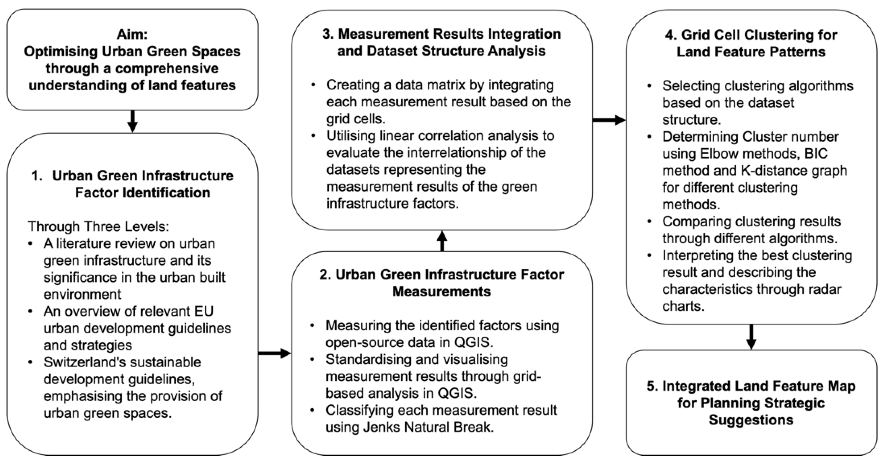
2.1. Methodologies and Framework

The objective of this study is to delineate and optimise the provision of urban green infrastructure, predicated upon a comprehensive understanding of its social, ecological, and environmental functions. This inquiry is structured around four key questions that will direct the analytical process as follows:

• What factors pertinent to the functions of urban green infrastructure, from various perspectives, should be considered in this study?
• How does the examined district perform in relation to these selected factors?
• What interrelationships exist among these identified factors?
• Furthermore, can the measurement outcomes of these factors be synthesised to provide a holistic characterisation of the land use situation from multiple viewpoints?
• In what ways can common patterns of land use situations be identified to inform strategic recommendations for enhancing the provision of urban green infrastructure within the studied district?

Consequently, this study was organised into five distinct phases (Figure 1). The initial phase identified the factors of urban green infrastructure from three perspectives. A brief literature review of the existing scholarship on the factors of urban green infrastructure and their significance within the urban built environment yielded the candidate factors from a scientific viewpoint. The subsequent selection of the involved factors was refined through adherence to the EU sustainable urban development guidelines and the Sustainable Development Strategies of Switzerland and Zurich 2030 in order to focus on the most relevant elements for the city redevelopment within the studied district. These selected factors were measured within a geographic information system (GIS) during the second phase. The findings were classified utilising the Jenks Natural Break method and visualised using a rectangular grid system, transforming polygon-based land use data into standardised grid cell information for enhanced comparison and integration.

The subsequent phase integrated the measurement results of each factor into a multi-variable data matrix based on the grid cells and examined the interrelations among these variables. Later, this study employed statistical algorithms to categorise grid cells into groups with similar characteristics, culminating in a clustering map of the studied area. The cluster centroids, representing the average values of each variable, illustrated the characteristics of the clusters through multi-dimensional radar charts. This methodology enabled this study to identify patterns in land features across the district, serving as a decision-support tool and offering valuable insights for optimising green infrastructure within the district for planners, designers, and policymakers.

2.2. Study Area

The district of Altstetten-Albisrieden is situated to the west of Zurich City, encompassing an area of 12.1 square kilometres, ranging from the Limmat River in the northeast to the Uetliberg mountains in the southwest (refer to Figure 2). The progression of the Altstetten-Albisrieden district over the past century exemplifies the patterns of urbanisation witnessed in Switzerland and across Europe. As a region bordering the central city, the overall development of this area is primarily attributable to the rapid industrialisation and the enhancement of infrastructure connecting the central city to its surrounding locales. Furthermore, during the 1980s, the flourishing economy and the escalating demand for improved living conditions rendered the district’s verdant landscape appealing, thereby stimulating residential developments aimed at delivering superior living conditions characterised by relatively low population and building densities. Such conditions highlight the significant potential for urbanisation driven by progressive redevelopment concentrating on densification, thereby necessitating critical considerations concerning the provision of urban green spaces within the modern built environment. A similar scenario is observable in the districts of Seebach and Oerlikon, situated in the northern region of Zurich. In contrast to other districts, the Altstetten-Albisrieden area exhibits a diverse topography marked by various geographical features, with railways at its core and mountains delineating its boundaries. As one of the earliest incorporated communities, Altstetten-Albisrieden displays a blend of architectural styles and urban forms, ranging from single-family homes to contemporary high-rise buildings, reflecting the evolution of urban development over time.

Currently, Altstetten is home to 34,098 residents, encompassing 18,059 housing units and 46,839 job opportunities, with 47% of the area developed and 28% designated as green space. In contrast, Albisrieden accommodates 22,412 inhabitants, 12,000 housing units, and 12,310 jobs, with 41% of the area developed and 43% covered by forest. In efforts to enhance green infrastructure in construction areas, this study excluded closed forests adjacent to the river and the mountain foothills from its analysis.

2.3. Urban Green Infrastructure Factors

Encompassing both global and Swiss regional contexts, a thorough examination of sustainable urban development strategies and guidelines underscores essential principles for Switzerland’s Green Urban Agenda. These principles underscore the significance of conserving urban nature and green spaces, ensuring the provision of high-quality open and public spaces, improving ecological livelihoods, promoting accessibility to public green areas and vital amenities within short distances from residential neighbourhoods, and fostering social inclusion while safeguarding natural resources [28].

The existing body of literature, focusing on addressing these principles, examines the functions of urban green infrastructure from varying perspectives. The advantages of regulating outdoor temperatures and mitigating the urban heat island effect in urban areas are evident through the extent of green surfaces and the quantity of greenery, which are widely acknowledged globally [4]. While the integration of substantial green spaces into urban environments generally enhances air quality, the highly context-dependent contributions of urban green infrastructure have been analysed through empirical simulation modelling and actual measurement. The structural configurations and density of buildings and vegetation significantly influence interactions with wind flows, thereby affecting the dispersion of air pollutants [29,30,31] and, consequently, impacting individual health [32,33,34]. Furthermore, they encourage the establishment of green paths and corridors that enhance ecological sustainability [8,35]. The spatial distribution of greenery, particularly the allocation of public green spaces within urban areas, which contributes to outdoor activities and social equity, is typically assessed through metrics of accessibility based on space size [17,36,37] alongside the types and density of vegetation [38,39].

Consequently, this study has identified six primary factors for the examination of urban green infrastructure. Quantity-based metrics, such as green surfaces and leaf area, assess the extent of greenery that covers the ground and vegetation canopies, thereby emphasising the quantity of greenery present within land use. Distance-based measures, including accessible public green spaces and total areas, evaluate the spatial distribution of public green areas in relation to district residents, reflecting human activities as well as considerations pertaining to social justice. Furthermore, the metric associated with land development intensity, characterised by the green ratio and connections, illustrates the support rendered to natural habitats and ecosystems.

2.4. Data

This study utilised relevant geo-information and data obtained from the City of Zurich’s open-access resources in 2021, which comprised building information, household locations, land use, and tree data. Updated building information detailing the number of households and job positions within each structure was acquired from the City of Zurich in 2023. Furthermore, this study employed street networks sourced from OpenStreetMap to analyse spatial connections and assess service coverage areas of public green spaces throughout the district.

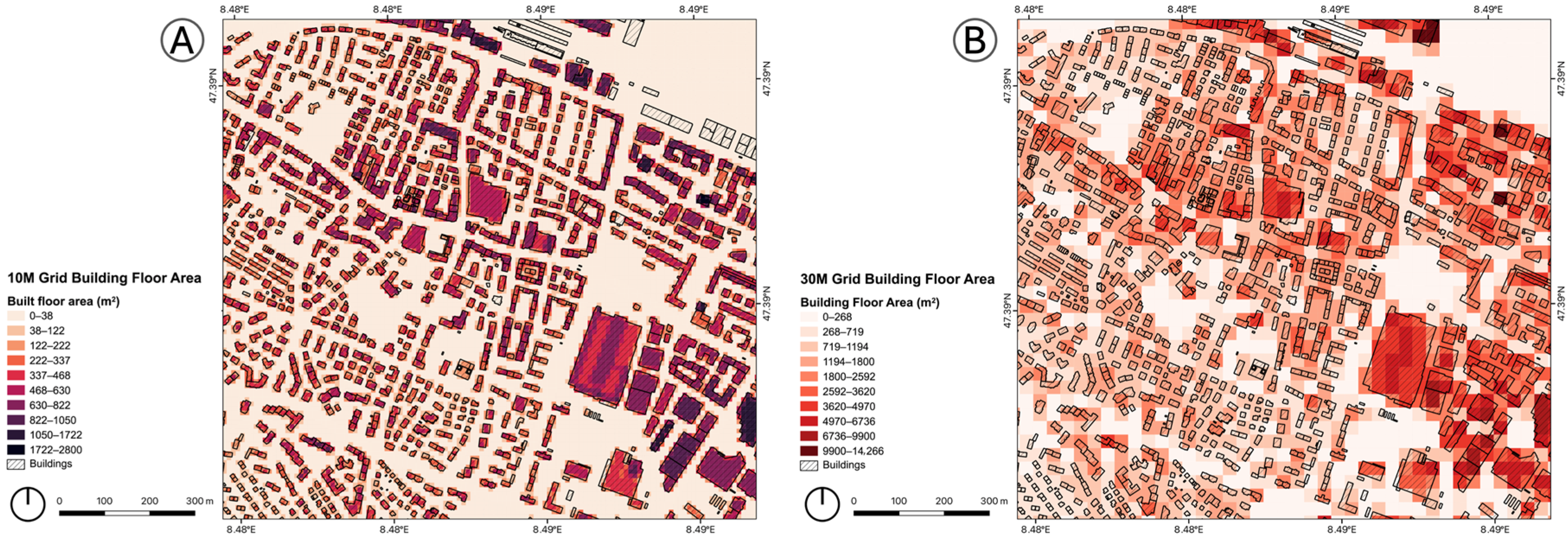
2.5. 10-m Rectangle Grid for Data Analysis and Visualisation

This study employed grid-based analysis to visualise, integrate, and cluster spatial data derived from various factors. This approach is particularly effective in managing continuous datasets and enhances the understanding of spatial phenomena across a given landscape [40]. It is acknowledged that grid size can significantly impact the analysis results [41,42,43]; thus, this study initially utilised a grid size of 30 m based on its achievement of the highest accuracy of 82.9% in the comparative analysis conducted by Lv et al. [44], slightly surpassing the performance of the 10-m and 15-m gride sizes. However, the 30-m grid was inadequate in delineating the general profiles of buildings and other spatial entities, and it also presented some misleading information in areas where building data were absent. This observation promoted the adoption of a grid size of 10 m, as recommended by N. Dong et al. [41], whose study evaluated the efficacy of various grid sizes in population distribution, ranging from 5 to 200 m. Figure 3 illustrates the distinctions between the 10-m and the 30-m grids concerning the representation of building floor areas within the study district.

Furthermore, the preference for grid-based analysis over direct use of land plots provided in the geo-information arises from several considerations as follows:

• A preliminary study examining buildings and developments within the district has revealed that numerous projects were strategically constructed across neighbouring land plots to maximise building volume and green spaces. Furthermore, certain land plots have been subdivided into multiple smaller segments to facilitate developments at various stages. These instances raised concerns that reliance solely on plot data derived from geo-information might fail to accurately capture the true distribution of green, grey, and built surfaces.
• In the assessment of the accessibility of public green spaces within the studied district, distinct segments of some specific large plot developments displayed discrepancies in both the quantity and size of accessible public green spaces, thereby complicating the data validation and clustering processes. In this context, the designated grid network served to standardise the measurement of the green factor across land units.
• Most buildings have direct connections to roads and streets, and land plots do not adequately group buildings or establish a coherent spatial hierarchy beyond individual structures. This is especially relevant when analysing accessibility to green spaces; thus, land plots are more suited to administrative purposes than to fostering spatial development.

Consequently, the 10-m rectangular grid partitioned the entirety of the studied area into 122,008 square units, of which 87,622 units were incorporated in the green factor measurement and clustering process of this study, excluding the forested regions located in the southern section of the district.

2.6. Methods and Application

2.6.1. Land Development

The land development analysis examined the constructed surface area and construction volume within the targeted regions. This included roadways, streets, railways, building footprints, and other impervious surfaces that were classified as constructed surfaces, along with building floor areas contributing to the overall construction volumes. The geo-information related to roadways, streets, railways, and other impervious surfaces was obtained directly from the City of Zurich, while the building floor areas were derived from the polygons representing building footprints, combined with the updated building floor counts as of 2023 provided by the City of Zurich.

2.6.2. Green Surface in Land Use

The essential geographical information regarding green spaces was derived from open-source data provided by the City of Zurich. These data include attributes such as polygon geometries and classifications of green spaces. Given that multiple plots within the district have experienced redevelopment over the past five years, on-site observations and Google Earth imagery were also used to update and verify the geographical information concerning these green areas.

2.6.3. Leaf Area

This study used the leaf area index (LAI) to assess the density of leaves within the district. The LAI is a critical metric in the field of climate change research [45]. It measures half the total intercepting area per unit of ground surface area [46] and quantifies the amount of leaf area in an ecosystem [45]. The leaf area calculation of this study consists of two parts: the ground green surfaces and the canopies of trees in the urban area. The green ground surfaces functioning as open spaces in gardens and parks and green landscape areas surrounding buildings, urban farming areas, and intensively cultivated fields were calculated as grasslands, gardening fields, and crop fields, respectively. The leaf area of tree canopies was determined using the particular LAI values along with tree information, such as canopy dimension and species information, provided by the City of Zurich.

A substantial body of research has examined and quantified the LAI values of various vegetation species, employing diverse methodologies and perspectives. Since LAI values can fluctuate significantly due to numerous factors affecting plants, such as cultivation conditions, age, season, life stages, and the methods of measurement [45], this study adopted LAI values, listed in Table 1, grounded in specific principles.

• The case study area encompasses over two hundred tree species. This study streamlined the information and categorised these species based on their respective vegetation genus and Latin nomenclature.
• Considering the impact of climate on vegetative growth, this study primarily selected LAI values from research conducted within temperate climate zones that closely resemble the studied area. In instances where specific LAI values were not available from the aforementioned research, this study utilised data from tropical zones, particularly referencing the vegetation database provided by EarthData, NASA, and the Flora & Fauna Web by Singapore National Parks.
• For tree species lacking available LAI values, this study adopted general LAI values pertinent to broadleaf and coniferous trees.
• In addressing the variations in canopy structure and leaf density across different life stages, particularly the seasonal fluctuations in deciduous trees, this study favoured LAI values corresponding to mature trees measured during the period of maximum foliage, typically from early summer to early autumn, with variations depending on plant species and cultivation techniques.
• Numerous studies have examined the divergence in LAI values among tree species attributable to the application of diverse measurement and calculation methods, including litter traps, Allometric methods, Digital Hemispherical Photography (DHP), and Tracing Radiation and Architecture of Canopies (TRAC) [45]. In such instances, this study preferred to utilise either the proposed LAI value from the existing research or the average values obtained from various measurement approaches.
• Urban farming zones are areas where vegetables and flowers are typically cultivated. This study applied the average LAI value for several common vegetables and flowers. The intensively cultivated fields within the case study recorded an LAI value of 2.9, referencing the statistics derived from the LAI dataset by region [47]. Furthermore, the LAI value associated with grassland is significantly correlated with the height of grasses and the species present within a given year. For the case study, the mean LAI value of 2.9 was utilised, as recorded in Italy during the summer months [48].

Table 1. Main tree species of the studied area (the information on tree species referred to the data from the Swiss National Forest Inventory [49] and tree information provided by the City of Zurich) and the leaf area index (LAI) values used in this study.

Category	Species	Leaf Area Index (LAI)
Tree	Spruce (Picea)	7.5 (It is the mean value of the results from three studies: a Litterfall study in 1998 with a result of 7.5, an LAI-2000 measurement result of 7.8 carried out in the summer of 2001 [50], and a study conducted in the Alpine biogeographic region suggesting a value of 7.28 [51].)
	Fir (Abies)	5.1 (The value referred to the three research measuring the LAI through the Litterfall traps method in the Southern Carpathian Mountains, Romania [52] and the mixed forest in Italy [53,54].)
	Larch (Larix)	3.6 (The study conducted in the Alpine biogeographic region suggested the mean value to be 3.61 [51].)
	Pine (Pinus)	5.7 (It is the mean value referring to the result of a study conducted in the forests of Spain [55].)
	Beech (Fagus)	5.5 (It is the mean value of the given LAI values ranging from 2.3 to 7.8 in the study conducted in Switzerland [50].)
	Maple (Acer)	4.0 (It is a suggested value by Cerny [56].)
	Ash (Fraxinus)	2.8 (It is a suggested value by Ladefoged [57] and used in the study conducted in the Czech Republic [58].)
	Oak (Quercus)	4.7 (It is a value used in the study in the Czech Republic [58].)
	Chestnut (Castanea)	2.5 (It is a measured value from June to October near the Botanical Garden of the University of Trieste, Italy [59].)
	Tilia (Tilia)	5.3 (It is a value used in the study in the Czech Republic [58].)
	Apple tree (Malus)	3.0 (Due to the variation of leaves at different growth stages throughout a year, the LAI value here refers to the mean values of the leaf differentiation growth stages through the ground-truth LAI measurements [60] and the mean value of the LAI measured from the middle of June to August in the study conducted in China [61].)
	Cherry tree (Prunus)	4.8 (Due to the different LAI values between different pear tree species, the value here referred to the average of the mean values of the original LAI of the Sweetheart cultivar and the Bing cultivar, measured in the study in Chile [62].)
	Pear tree (Pyrus)	1.7 (This value referred to the mean value of the measured LAI values in the study conducted in China [63].)
	Mulberry (Morus)	3.1 (This value referred to the mean value of the actual LAI of the six mulberry trees in the study by Peper and McPherson [64].)
	Walnut (Juglans)	6.3 (This is the mean value of the LAI among three monocultures of black walnuts in six different years during 1979–2003 in Sikenica, Slovakia [65].)
	Willow (Salix)	3.3 (This is the mean value measured in the study by Tharakan et al. [66].)
	Broadleaf	4.0 (This is the mean value mentioned in the review by Parker [67].)
	Conifer	5.2 (Ibid.)
Urban farming/gardening fields		3.2 (The LAI value refers to the four types of common vegetables, Tomato (4.2), pepper (3.3), and cucumbers (3.6), measured directly by the study in Turkey [68]; the optimal LAI value of eggplants in August is 3.3 [69] and the common cutting flowers, such as rose (a measured LAI of 3.0 around August) [70], chrysanthemum (a mentioned value range of 2.7–3.5) [71], tulip (a measured value range of 1.7–2.4) [72], and lily (a measured LAI value of 2.6) [73].)
INTENSIVE CULTIVATED FIELDS		2.9
Meadow		2.9

Table 1. Main tree species of the studied area (the information on tree species referred to the data from the Swiss National Forest Inventory [49] and tree information provided by the City of Zurich) and the leaf area index (LAI) values used in this study.

Category	Species	Leaf Area Index (LAI)
Tree	Spruce (Picea)	7.5 (It is the mean value of the results from three studies: a Litterfall study in 1998 with a result of 7.5, an LAI-2000 measurement result of 7.8 carried out in the summer of 2001 [50], and a study conducted in the Alpine biogeographic region suggesting a value of 7.28 [51].)
	Fir (Abies)	5.1 (The value referred to the three research measuring the LAI through the Litterfall traps method in the Southern Carpathian Mountains, Romania [52] and the mixed forest in Italy [53,54].)
	Larch (Larix)	3.6 (The study conducted in the Alpine biogeographic region suggested the mean value to be 3.61 [51].)
	Pine (Pinus)	5.7 (It is the mean value referring to the result of a study conducted in the forests of Spain [55].)
	Beech (Fagus)	5.5 (It is the mean value of the given LAI values ranging from 2.3 to 7.8 in the study conducted in Switzerland [50].)
	Maple (Acer)	4.0 (It is a suggested value by Cerny [56].)
	Ash (Fraxinus)	2.8 (It is a suggested value by Ladefoged [57] and used in the study conducted in the Czech Republic [58].)
	Oak (Quercus)	4.7 (It is a value used in the study in the Czech Republic [58].)
	Chestnut (Castanea)	2.5 (It is a measured value from June to October near the Botanical Garden of the University of Trieste, Italy [59].)
	Tilia (Tilia)	5.3 (It is a value used in the study in the Czech Republic [58].)
	Apple tree (Malus)	3.0 (Due to the variation of leaves at different growth stages throughout a year, the LAI value here refers to the mean values of the leaf differentiation growth stages through the ground-truth LAI measurements [60] and the mean value of the LAI measured from the middle of June to August in the study conducted in China [61].)
	Cherry tree (Prunus)	4.8 (Due to the different LAI values between different pear tree species, the value here referred to the average of the mean values of the original LAI of the Sweetheart cultivar and the Bing cultivar, measured in the study in Chile [62].)
	Pear tree (Pyrus)	1.7 (This value referred to the mean value of the measured LAI values in the study conducted in China [63].)
	Mulberry (Morus)	3.1 (This value referred to the mean value of the actual LAI of the six mulberry trees in the study by Peper and McPherson [64].)
	Walnut (Juglans)	6.3 (This is the mean value of the LAI among three monocultures of black walnuts in six different years during 1979–2003 in Sikenica, Slovakia [65].)
	Willow (Salix)	3.3 (This is the mean value measured in the study by Tharakan et al. [66].)
	Broadleaf	4.0 (This is the mean value mentioned in the review by Parker [67].)
	Conifer	5.2 (Ibid.)
Urban farming/gardening fields		3.2 (The LAI value refers to the four types of common vegetables, Tomato (4.2), pepper (3.3), and cucumbers (3.6), measured directly by the study in Turkey [68]; the optimal LAI value of eggplants in August is 3.3 [69] and the common cutting flowers, such as rose (a measured LAI of 3.0 around August) [70], chrysanthemum (a mentioned value range of 2.7–3.5) [71], tulip (a measured value range of 1.7–2.4) [72], and lily (a measured LAI value of 2.6) [73].)
INTENSIVE CULTIVATED FIELDS		2.9
Meadow		2.9

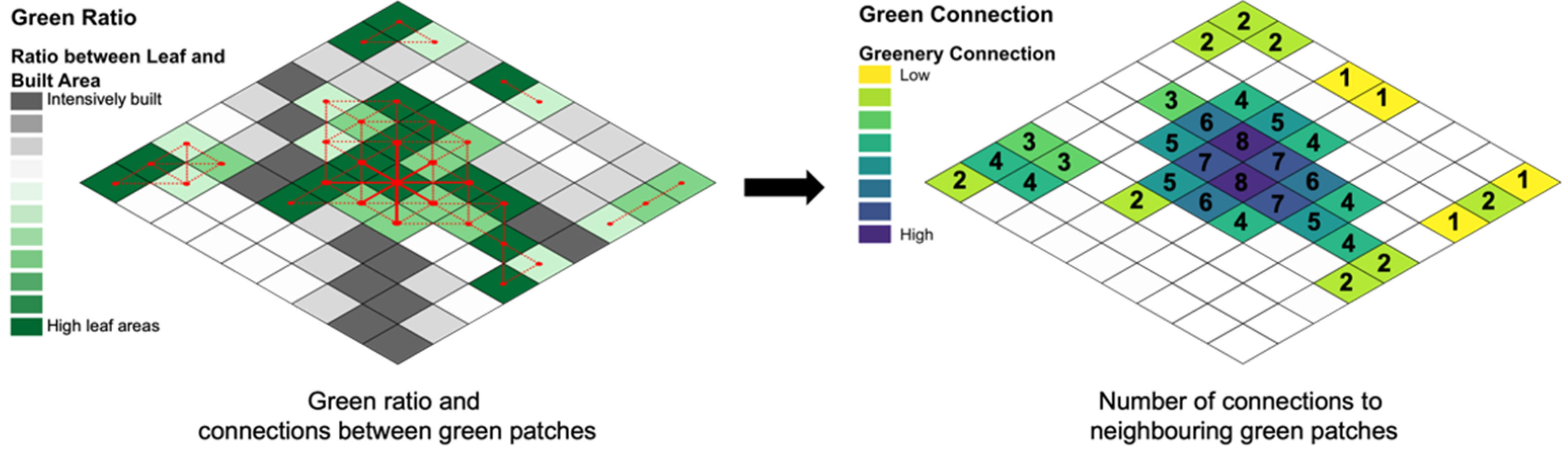
2.6.4. Green Ratio and Connection Measurement

The ongoing growth of the human population and the expansion of urban areas, characterised by buildings and infrastructure, have led to the overexploitation of natural resources and posed significant threats to natural habitats [74]. Habitat fragmentation occurs when larger, interconnected habitat areas are divided into smaller, isolated patches due to human development, infrastructure, and natural processes. This fragmentation poses serious challenges to landscape connectivity, which is crucial for biodiversity and climate stability [74,75,76].

This study introduces the green ratio as one perspective on how the development in the studied district facilitates or impedes animals’ movement among green patches. Opposed to the concept of landscape resistance [77,78], the green ratio indicates the impacts of environmental factors on natural habitat movement and ecosystems. A high green ratio implies easy movement across patches, while a low ratio represents limited movement or a barrier to movement.

Referring to the de-fragmentation concept given by the Singapore National Parks Abroad (NParks) and its categorisation of spatial resistance in urban areas, the calculation of the green ratio in this study used the ratio between the leaf and built areas to indicate the facilitation level from intensive developed areas to high-quality green areas, including environmental variables such as land use (e.g., green landscape and grey landscape), roads and streets, human development (e.g., buildings and other structures), and leaf areas as follows:

$$\mathrm{Green} \mathrm{Ratio} ={\displaystyle \frac{\mathrm{Total} \mathrm{Leaf} \mathrm{Area} \mathrm{of} \mathrm{Green} \mathrm{surface} \mathrm{and} \mathrm{Vegetation}}{\mathrm{Total} \mathrm{Area} \mathrm{of} \mathrm{Building} \mathrm{Floors}, \mathrm{Grey} \mathrm{Surface}, \mathrm{Infrastructure} \mathrm{and} \mathrm{Road} \mathrm{Area}}}$$

In accordance with the concept of de-fragmentation, which entails the establishment of green pathways or corridors to connect fragmented green spaces or landscapes, this study utilised the analytical tool Distance Matrix within QGIS 3.40 Bratislava to discern the connections of each patch possessing a specific green ratio (green ratio > 0.1 in order to guarantee the amount of greenery in the grid patch) to its neighbouring green surfaces and vegetation, indicated in Figure 4. This analysis highlights potential green connections within the district.

2.6.5. Assessment of Public Green Spaces Accessibility

This study examined the social implications of green spaces in relation to their accessibility. It predominantly focused on publicly accessible green spaces, including city parks, gardens, open green spaces, and sports fields, under the ownership of the municipality. The analysis was organised around two critical factors: the number and total area of accessible public green spaces situated within an 800-m walking distance.

The methodology utilised in this study employs a centroid point or entrance when the dimensions of the space exceed 400 m to represent the geographical location of each public green space. By integrating the street network, the 800-m service catchment areas are delineated through vector processing tools, specifically employing Service Area and Hull functions within QGIS. The count of overlapping service areas reflects the number of accessible public green spaces. Given the diverse range of spatial dimensions of public green spaces across the studied district, this study further correlates the number of accessible public green spaces with their respective sizes to evaluate the total area of accessible public green spaces across various segments of the district. This analysis indicates the usage density of public green spaces and assesses the equity of their allocation.

2.6.6. Data Clustering Based on the Multiple Parameters of Green Space

The objective of this study was to systematically analyse the land features and their patterns, thereby structuring the classification of land areas based on their similarities related to green factors. Accordingly, clustering methods were selected to examine the dataset derived from the seven measured factors. The data clustering process commenced with an evaluation of the data distribution across each factor and the relationships among those factors pertinent to urban green infrastructure. Initially, the information regarding the measured factors was standardised and consolidated into their respective grid cells, aggregating all cells into a comprehensive data matrix. The Pearson Correlation Coefficient analysis was utilised to evaluate the linear relationships among the factors.

The data matrix was characterised by high dimensionality and identified the K-Means clustering method as the principal approach. However, the distribution of the dataset, represented within a three-dimensional coordinate system exhibiting varying density, highlighted the applicability of the Density-Based Clustering method (DBSCAN), the Hierarchical DBSCAN method (HDBSCAN), and the Gaussian Mixture Model (GMM) in conjunction with Principal Component Analysis (PCA). In order to execute the K-Means algorithm, this study utilised the Elbow Method to ascertain the optimal number of clusters (K value) for the algorithm, and the Bayesian Information Criterion (BIC) was applied to determine the suitable number of clusters. The optimal K value was subsequently employed within the K-Means clustering methodology to distinguish the datasets into discrete clusters. Simultaneously, the two critical parameters, epsilon (eps) and the minimum number of data points necessary for the algorithms of the DBSCAN and HDBSCAN algorithms, were established through the K-distance graph. The GMM algorithm does not necessitate any predetermined parameters; however, PCA analysis can significantly enhance the efficacy of clustering outcomes by reducing dimensionality. The results derived from all methodologies were projected for comparison within the studied area utilising QGIS. The Dunn index was employed to assess the quality of the clustering results.

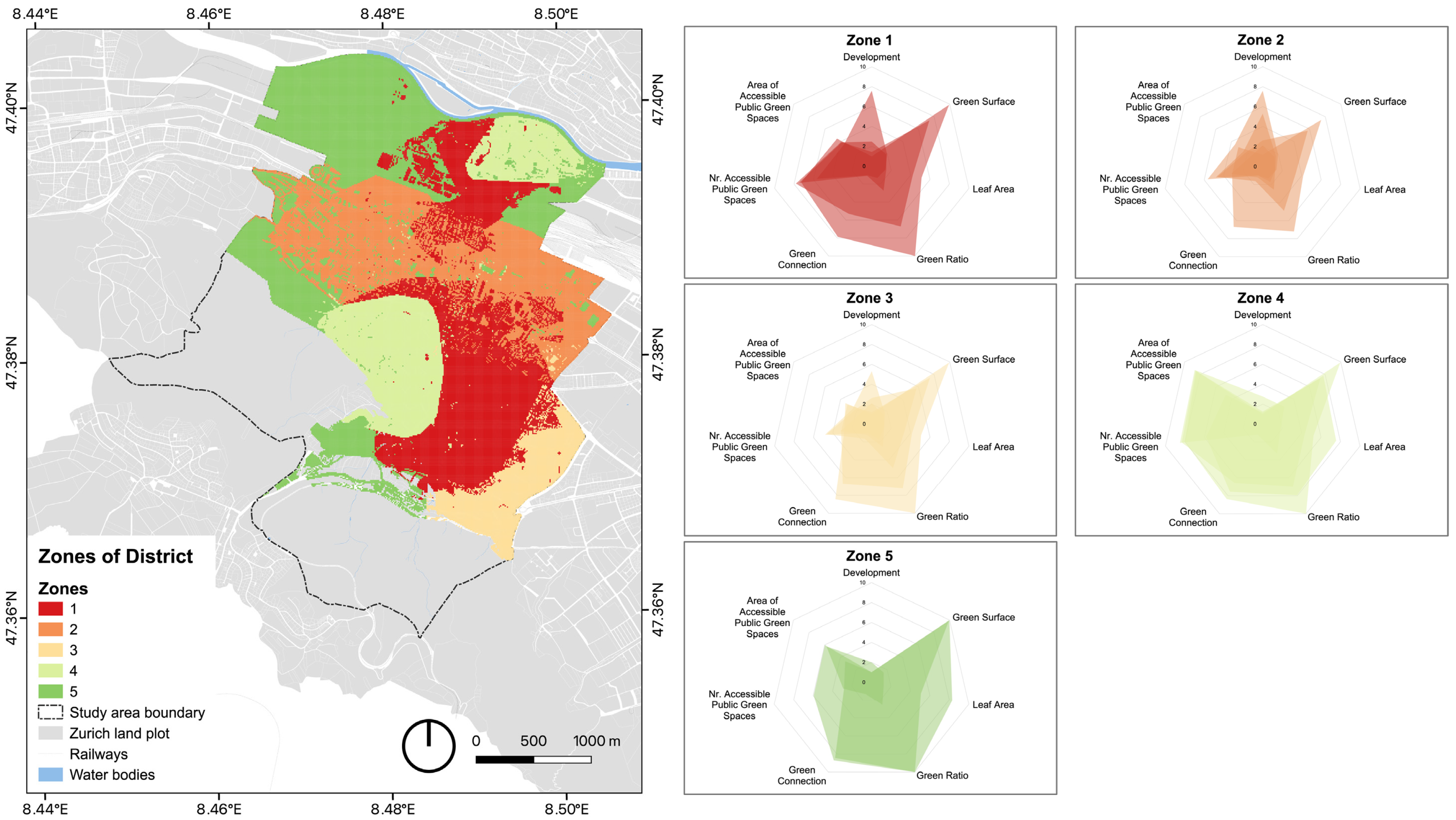
2.6.7. Classification for Feature Description

To elucidate the overarching characteristics of the factors associated with each cluster, this study employed the Jenks Natural Break classification method in order to categorise the dataset pertaining to each measured factor into ten distinct classes. This methodology effectively organises the data into classes that minimise the within-class variance while maximising the between-class variance during the calculations [79]. The centroid of each cluster with the mean values of the factor classes was utilised to produce radar charts that visually represent the distinctive characteristics of each cluster.

3. Results

3.1. Land Development and Greenery Availability

The subsequent figures (Figure 5A–C) present a comprehensive land development, green space, and leaf area analysis. As the colour gradient darkens within each figure, it indicates an increased concentration of measured factors within the respective grid cells. These figures illustrate the extent of land development, while areas characterised by intensive development and high-density buildings, particularly along railway lines and in the eastern sector of the district, are represented by grey surfaces. In contrast, residential areas feature only essential pathways for vehicular and pedestrian movement, thereby preserving substantial ground surfaces dedicated to green spaces. Beyond the green spaces, immediate surrounding buildings, public gardens, sports fields, urban gardening plots, and cultivated fields situated at the periphery make a significant contribution to the overall availability of green spaces. Given that the majority of green areas within the urban environment are adorned with turf and shrubs, the leaf area across the district remains relatively consistent. However, the presence of trees in public gardens, sports fields, and other open spaces provides a contribution of notably high leaf area values. On average, the mean value of development within each grid cell encompasses approximately 130 m², while the corresponding green surface measures about 46 m², and the average leaf area for the grid cells attains 160 m².

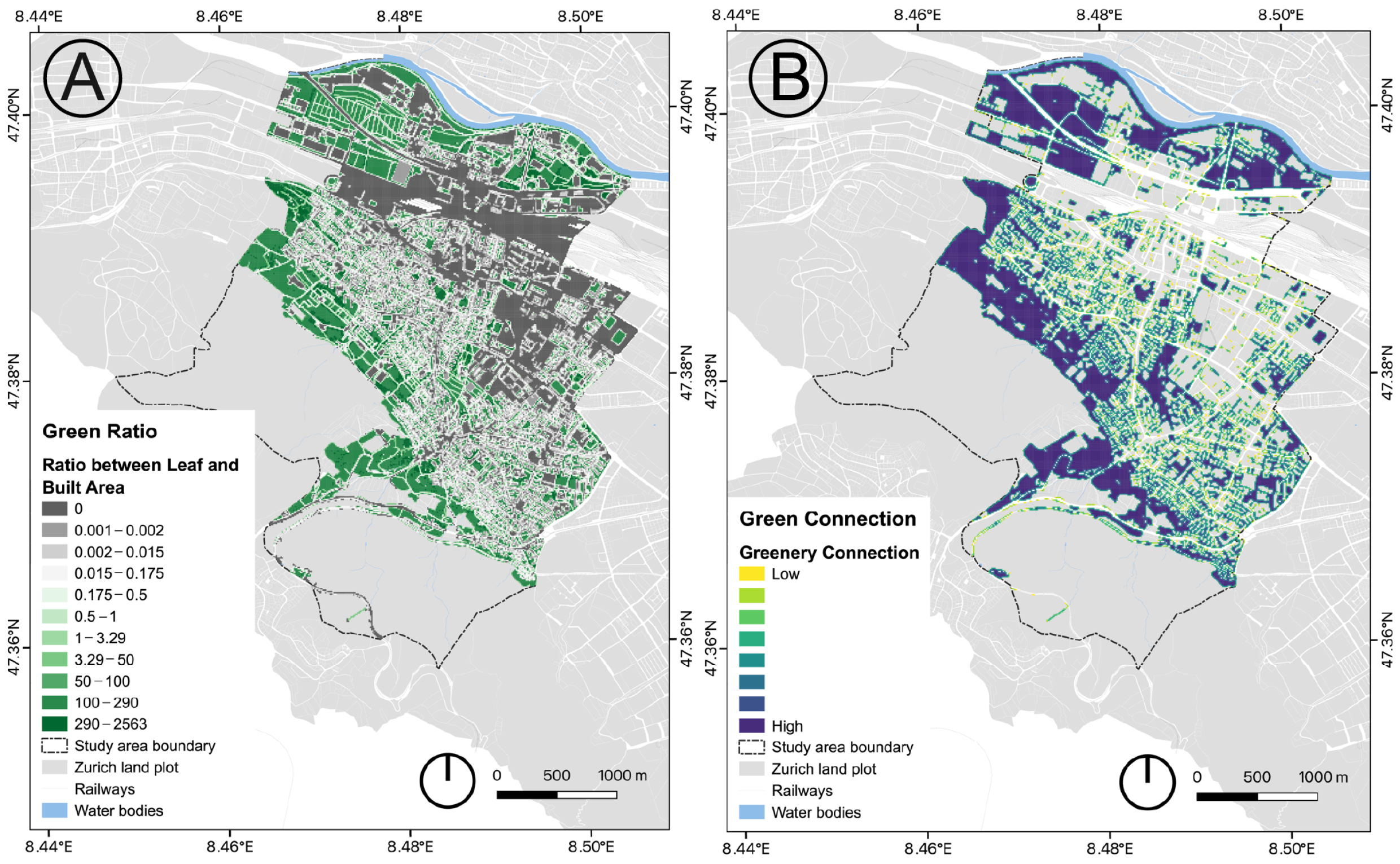
3.2. Green Ratio and Green Connection

The green ratio (Figure 6A) and the green connection (Figure 6B) generated through the distance matrix analysis reveal the impact of urban development on the fragmentation of natural habitats. The colours in the green ratio, ranging from dark green to dark grey in the spatial resistance, indicate that the grid units are becoming increasingly ineffective in restoring natural habitats or impeding the movement of organisms. Additionally, the grid cells in the green connections, differentiated by colours from yellow to dark purple, show a rise in connections with the surrounding cells. Both figures demonstrate that public gardens, urban gardening plots, sports fields, and cultivated areas play vital roles in fostering green connections. The heavily developed infrastructure and high-density buildings create significant gaps in the urban greenery stretching from the Limmat River to the Uetliberg foothills. Moreover, these intense developments, buildings, and street networks fragment the greenery in the built-up area into scattered and isolated small patches, diminishing its capacity for natural recolonisation.

3.3. Accessibility of Public Green Spaces

The accessibility of public green spaces is evaluated through the lens of two primary factors: the number of public green spaces located within an 800-m walking distance (as illustrated in Figure 7B) and the aggregate area of those spaces (as depicted in Figure 7C). The gradient of colours, transitioning from dark to light green in both figures, signifies a decline in the availability of accessible public green spaces as well as a reduction in the cumulative area of these spaces. In general, the geographical distribution of the existing public green spaces guarantees that each household within the studied district can reach at least one public green space within an 800-m radius. However, households situated in the central area and adjacent to the Limmat River have access to over ten public green spaces within the same distance, irrespective of the size of these areas. Moreover, taking into account the dimensions of each public green space, households located in the northeastern and southwestern regions are able to utilise significantly larger green spaces compared to those in other areas. Conversely, households in the central–western portion of the district are disadvantaged in both aspects, underscoring the necessity for the introduction of additional public green spaces in this area.

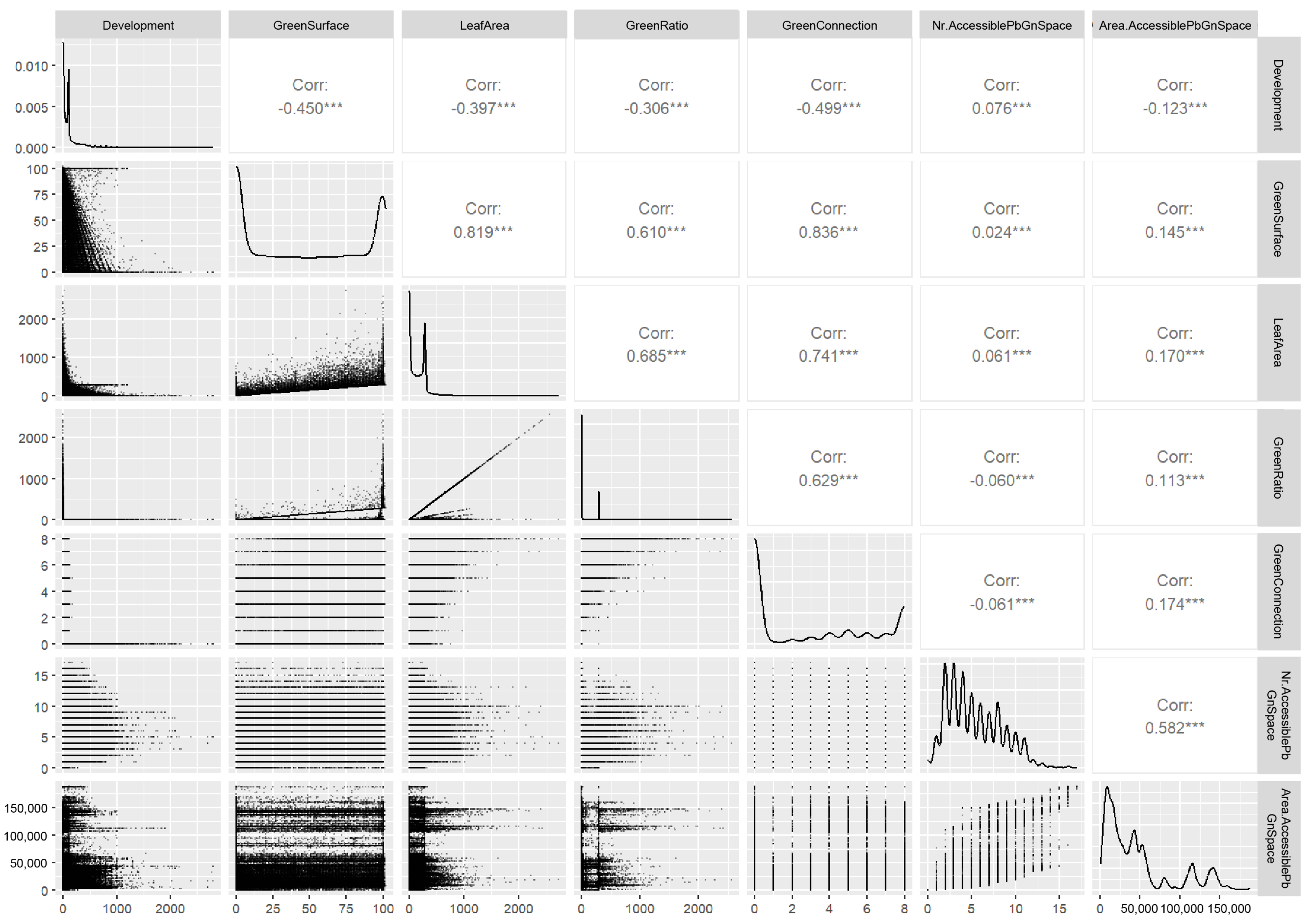
3.4. Interrelationships Among Measured Factors

In the process of compiling the measured factors as variables for the examination of their interrelationships, the results depicted in Figure 8 reveal significant positive linear relationships among the factors pertaining to green surface, leaf area, and green connection at the α = 0.001 level. This observation indicates a direct correlation whereby an increase in green surface positively influences both the enhancement of leaf area and the improvement of green connection within grid cells. Furthermore, the linear relationships between the green ratio and the factors of green surface, leaf area, and green connection are observed to be moderately positive, akin to the relationships between the two factors that pertain to the accessibility of public green spaces. Notably, the development factor reflects a negative correlation with most other factors; nonetheless, the correlation coefficient values remain from very weak to moderately high. Additionally, the two factors associated with public green space accessibility exhibit independence from others, as evidenced by the very low correlation coefficient values between them.

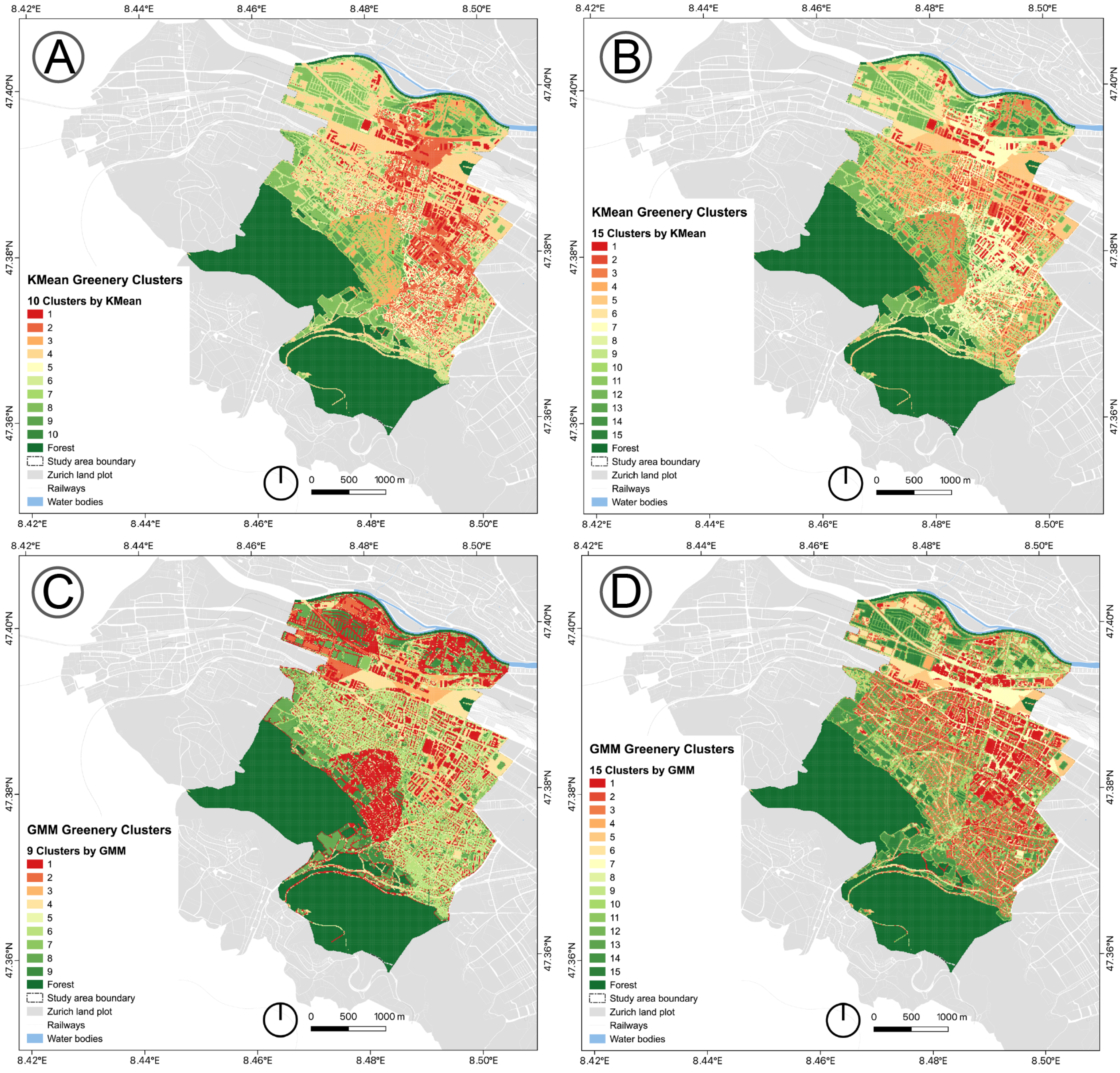
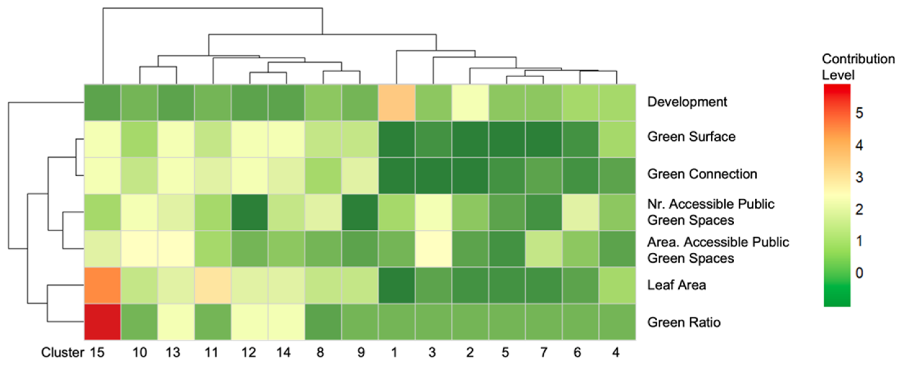
3.5. Green Feature Clustering

The distinctive feature of the comprehensive dataset comprising green attributes is characterised by high dimensionality, 87,622 observations encompassing seven factors. The Elbow Method recommends that the optimal K value is around 10 to 15 (Figure 9A). The intricacy introduced by the seven dimensions resulted in a continuous increase in values across all Bayesian Information Criterion (BIC) models, in conjunction with the escalation of the K value. Due to certain variables exhibiting strong linear correlations, this study implemented the PCA method to reduce the dataset’s dimensionality, ultimately retaining four principal components that achieved cumulative variances of 90%. Nevertheless, this dimensionality reduction did not enhance the results from either the Elbow Method or the BIC, suggesting a similar K value range for clustering (Figure 9B).

In trials with varying combinations of the two parameters, the eps value and the minimum points of the cluster, the DBSCAN and the HDBSCAN algorithms generated clusters of no more than six, with extremely uneven data points distributed in each cluster, implying the method is unsuitable for this dataset. The GMM algorithm based on the PCA reduced-dimensional dataset resulted in nine clusters applying the “VVE” model for the minimum request of BIC. Since the BIC algorithm verified that fifteen clusters with the “VEV” model performed better than in the other situations earlier (Figure 9B), the GMM was also forced to cluster the dataset into fifteen groups through the “VEV” model specifically. Figure 10 displays the clustering results of the six methods, projected in a three-dimensional system.

The four results of clustering—ten and fifteen clusters derived from the K-Means, nine clusters utilising the “VVE” model, and fifteen clusters employing the “VEV” model as per the GMM technique—are illustrated in Figure 11 for the district under study. In order to facilitate a comparative analysis of the differences among these clustering results, all clusters have been systematically organised in descending order based on average measurements of the development factor. The two outcomes from the K-Means adeptly differentiated between grid cells associated with buildings, grey surfaces, and green surfaces. A notable distinction between the 15-cluster K-Means outcome and the 10-cluster K-Means outcome is that the former delineated grid cells characterised by low development into three distinct groups, informed by their green surface, green ratio, and accessibility to public green spaces. In contrast, the GMM algorithm exhibited inferior performance relative to the K-Means method; both outcomes from the GMM faced challenges in effectively segregating buildings from green or grey surfaces and resulted in a dispersed distribution of points around green areas. This comparison was, moreover, verified by the Dunn index, as shown in

Table 2. Dunn index of the four clustering results. The higher the index value, the better the clustering result.

	Dunn Index
10 Clusters by K-Means	0.054
15 Clusters by K-Means	0.060
9 Clusters by GMM	0.037
15 Clusters by GMM	0.036

, where the 15-cluster K-Means outcome obtained a higher score than the rest, indicating a better compactness or goodness of clustering. The 10-cluster K-Means result received a slightly lower score.

Upon the division of each measured factor into ten distinct classes utilising the Jenks Natural Break methodology, this study employed the average values of these classes to accurately represent the characteristics of the fifteen clusters as identified by the K-Means clustering method. Figure 12 illustrates that Clusters 1 and 2 are predominantly composed of densely constructed areas within the district, characterised by a minimal presence of green surfaces and leaf areas. Households located within these two clusters have access to over five public green spaces; however, these areas are relatively small in size. Clusters 3 and 4 encompass moderately constructed areas, distinguished by their respective access to green spaces. The former benefits from commendable access to extensive public parks, despite having limited private green surfaces. In contrast, the latter contains significant private green surfaces within each grid cell, though it offers lesser access to public green spaces. While not extensively developed, the grid cells within Clusters 5 to 7 exhibit restricted green surfaces and leaf areas, indicating a predominance of grey surfaces. The regions encompassed within Clusters 8 to 11 feature a majority of surfaces adorned with vegetation, thus facilitating green connections within the constructed environment. Clusters 12 to 15 comprise green surfaces that fulfil various ecological functions, with distinctions arising from the types of vegetation present and their relational dynamics with other public green spaces.

Based on the identified clusters and their specific combinations, the studied area was systematically divided into five principal segments (see Figure 13). The central areas, classified as the first zone, extend vertically from north to south and are characterised by Clusters 1, 7, 8, and 13. The second zone, positioned in the middle of the district, elongates horizontally along the railway lines from east to west, comprising Clusters 1, 2, 4, 5, and 9. In between the studied district and its eastern neighbouring region lies the third zone featured by Clusters 2, 4, 5, 9, and 12. Two aggregations of Clusters 3, 10, 11, and 14, which constitute the third zone, are located in proximity to the Limmat River and the foothills of the mountains. The fourth zone, encompassing Clusters 6, 12, and 15, is situated in the peripheral region of the district.

The characteristics of each zone suggest potential strategies for land development. Zones 1, 2, and 3, being significantly densely constructed regions, face disadvantages due to their limited leaf areas and inadequate portions of accessible public green spaces. Consequently, proposed improvements prioritise the planting of additional trees and the expansion of public green spaces. As the majority of plots have been utilised for development, establishing community gardens and green spaces within these developments may alleviate the congestion experienced in public parks and gardens. Additionally, integrating structures for cultivating greenery would enhance aspects such as the green ratio and connectivity. The residential environment in Zone 4 is exemplary in terms of the availability of green spaces; hence, further investment in greenery may not yield substantial benefits for this area. Nonetheless, this zone may serve as a resource for future development due to its relatively lower building density, assisting in alleviating the pressures of rising population density. Finally, Zone 5 functions as a buffer between urbanised areas and the natural environment.

4. Application in the Lindenplatz Subsite

This study employed the 400-m service catchment area of Lindenplatz, encompassing an area of 0.5 km², located at the centre of the district, as a representative subsite for the optimisation of green infrastructure. This subsite comprises a diverse array of structures, including residential buildings, shopping centres, office buildings, educational institutions, and places of worship. It serves as a crucial cultural and commercial hub for the entire district.

As illustrated in Figure 14A, this subsite case traverses Zones 1 and 2 and is deemed appropriate for the general improvement suggestions proposed in the preceding session. A detailed examination of the subsite is provided in Figure 14B. In conjunction with the densely developed areas (Cluster 1 and Cluster 2) within the subsite, the upper half of the site is predominantly characterised by streets and other grey surfaces (Clusters 4 through 6), interspersed with smaller green patches (Clusters 8 and 9). In contrast, the lower half of the site reveals an increase in the prevalence of green spaces displaying superior features (Clusters 10 and 11), which connect to four substantial patches (Clusters 12, 13, and 14). In light of the aforementioned circumstances, the comparatively intensive developments and buildings present significant obstacles to the provision of additional green surfaces and the connectivity of green spaces at ground level. The strategies for optimising the green infrastructure of the site emphasise the enhancement of green spaces and leaf areas by utilising existing building structures for vegetation, such as roof gardens and green facades.

Given that grid size can significantly affect the analysis of geospatial information and the interpretation of the results, determining the appropriate grid size for both data analysis and visualisation has emerged as a primary challenge of this study. As an initial investigation aimed at evaluating the feasibility of the analytical process, a rectangular grid measuring 30 m by 30 m was utilised to generate a comparatively smaller dataset. The entire analytical procedure, which includes the measurement of green factors and subsequent clustering, concluded with the identification of ten clusters, as illustrated in Figure 14C. The findings indicate a more abstract pattern closely associated with the ten clusters identified using the K-Means algorithm, although the profiles of buildings, streets, and other spaces appear somewhat obscured. At the district scale, this outcome illustrates a comprehensive pattern of land features, highlighting the continuous patches of densely developed areas that benefit from their proximity to a wealth of public green spaces in the city centre, alongside the relatively homogeneous low-density areas interspersed with green surfaces. When examining the neighbourhood scale, with Lindenplatz and its 400-m service catchment area as an illustrative example (Figure 14D), the clustering based on a 30-m grid underscores the interpretation of two primary components: the upper section characterised by dense development and the lower section showcasing green surfaces. Variations in clustering outcomes between the 10-m and 30-m grids suggest that different grid sizes are suited to various scales of analysis and their corresponding objectives. A larger grid size, manifesting in continuous patches, facilitates decision-making strategies at the city scale, while a smaller grid size allows for a more thorough investigation at the neighbourhood scale.

5. Discussion

The objective of this study was to synthesise the analysis of urban green infrastructure with the intention of generating land feature patterns that would inform strategic recommendations aimed at enhancing the provision of local urban green spaces, grounded in a comprehensive understanding at the district scale. In alignment with this objective, this study examined green factors from both social and ecosystem perspectives within a 10-m grid, clustering the grid cells into fifteen groups characterised by distinctive land features. The findings revealed five zones within the studied district and provided insights into specific urban green strategies customised for each zone. Throughout the entire examination and integration process, some issues related to data collection and analytical methods emerged as significant considerations for future development.

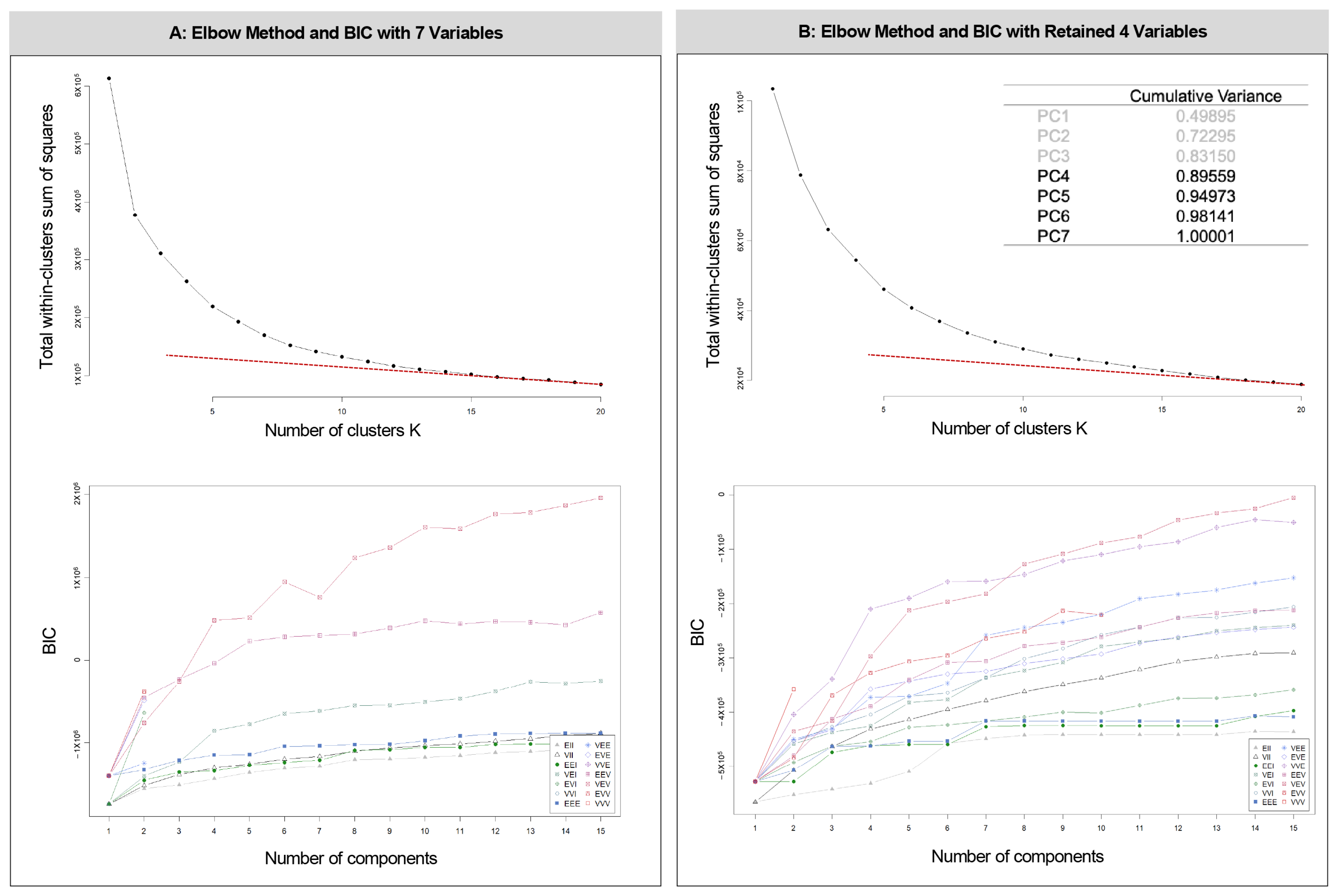
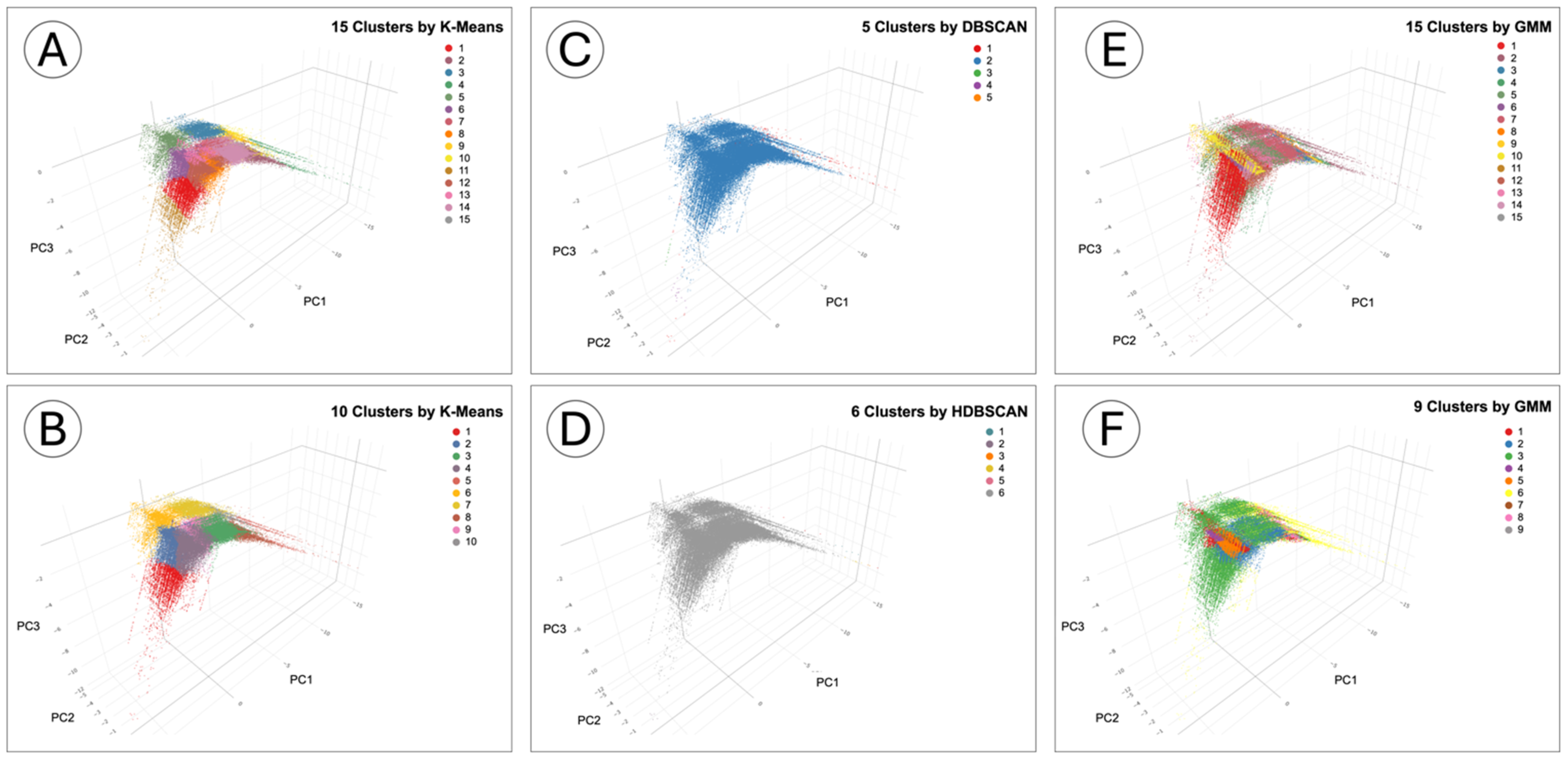
5.1. Clustering Process and Results

As delineated in Figure 10, the distribution of the PCA-reduced dimensional dataset and the outcomes from the six clustering algorithms indicated certain characteristics of the land use and urban green infrastructure within the examined region. Generally, the dataset exhibited a distinct U–shape within the three-dimensional coordinate system. The three prominent surfaces across various two-dimensional systems signified two primary types of grid cells, each exhibiting a predominant factor. By integrating the seven-dimensional radar charts of each cluster, this prevailing characteristic appears to be the green ratio, which reflects the balance between development and greenery in each grid cell. Notably, both the DBSCAN and HDBSCAN algorithms classified the majority of the dataset as a single cluster rather than dividing it into three, suggesting that the density of the data distribution was relatively homogeneous and continuous, showing minimal differentiation. The results from the DBSCAN and HDBSCAN demonstrated a smooth variation in spatial configuration, devoid of abrupt changes. Furthermore, these findings provided an indication for evaluating the spatial consistency and coherence of the urban area; however, a more sophisticated methodology and approach necessitate careful development. The K-Means algorithm effectively captured additional nuances of the dataset distribution, including the curvature of surfaces and certain ambiguous gaps present within each surface. Consequently, it produced superior clustering outcomes compared to the Gaussian Mixture Model (GMM) methods.

Stemmed from the fact that both the K-Means and GMM algorithms cluster a dataset from the random initialisation of centroids, one of the key challenges encountered during the clustering process was the variability in cluster assignments across different runs, which led to some different cluster configurations at the beginning. This study employed the alternative technique K-Means++ to stabilise the clustering by improving centroid initialisation. However, variability still remains a concern, especially when the dataset contains considerable overlapping points within a high-dimensional structure. Similarly, the GMM method, investigating the probabilities of each data point belonging to a particular cluster, is sensitive to the initial parameters and results in different cluster assignments between runs. The Expectation–Maximisation (EM) algorithm used in the GMM method can converge to varied local optima depending on initialisation and cause the reduction in stability. This challenge required multiple runs of the algorithm and strategies of carefully selecting the initialisation to obtain better consistency.

In addition to the nature of the algorithms, some other factors can also influence the stability of the cluster assignments, for instance, the number of clusters (K value) and the size and shape of the dataset. Theoretically, clustering a larger dataset through the K-Means algorithm with any K values can achieve a more stable result than clustering a smaller dataset; on the other side, datasets with more dimensions and an unsymmetric structure lead to an increase in the instability of clustering [80]. The intricacy of these influential factors in the algorithm leads to the consideration of a better clustering procedure to enhance the robustness of the outcomes for future deep learning and further application extending to different urban contexts.

5.2. Contribution of Green Factors to the Clustering Process

In the process of clustering, each standardised measured factor contributed uniquely to the formation of clusters (see Figure 15). The primary observation indicates that with the exception of the development factor, the measured factors predominantly influenced Clusters 8 to 15, contributing significantly to their defining characteristics compared to the other clusters. Cluster 15 is particularly notable due to the exceptionally high contributions of the green ratio and leaf area. This variation in contributions also reflects the hierarchy among the measured factors as well as among the fifteen clusters throughout the clustering process, which may assist in facilitating spatial ranking as objective weights.

5.3. Grid-Based Analysis vs. Actual Land Plots

One of the primary concerns of this study was the utilisation of grid-based analysis rather than employing the designated land plot units during the assessment of the green factor and the clustering analysis. While the benefits of using the grid for standardising land information and datasets in the clustering process are apparent and advantageous, the drawbacks are also considerable from two perspectives. As noted in the preceding section, modifications to the grid size directly influence the interpretation of land feature patterns; thus, a meticulous selection of the grid size must correspond with the scales of this study, necessitating further exploration of the discrepancies in data accuracy and representation associated with the actual conditions arising from the implementation of different grid sizes. Moreover, the grid partitioned the actual land plots into smaller units, thereby somewhat constraining this study to an empirical level and leading to a loss of a comprehensive overview of each land plot that could have more effectively informed urban redevelopment initiatives. The subsequent step involves investigating methods to enhance the direct applicability of this study for practical urban planning strategies.

5.4. Green Ratio and Connection

Research on landscape resistance and connectivity has garnered increasing recognition as significant parameters influencing long-term biodiversity conservation. Nevertheless, a universally accepted methodology for systematically quantifying and modelling connectivity and resistance remains elusive [75,81]. This challenge arises from various factors, including the difficulties associated with observing animal movement, behavioural variations linked to specific species, and the fluctuations of environmental variables. This study, which does not identify the specific organism species present in the district, concentrated on the propensity of grid cells from two perspectives: leaf areas representing both the green surfaces on the ground and the tree canopies that facilitate animal movement and gene flow alongside the development characterised by impervious surfaces, infrastructure, roads, and buildings that perform as obstruction to movement continuity. To a certain degree, the comparison between these two perspectives, denoted by the green ratio, overlooks the differentiation between “isolation-by-distance” and “isolation-by-barrier”, as articulated by Zeller et al. [78]. For example, grid cells exhibiting an identical low green ratio may display either extensive grey surfaces coupled with minimal green surfaces on the ground (such as concrete surfaces) or consist of towering structures and trees (like high-rise buildings). However, the former scenario hinders movement, whereas the latter situation presents obstacles to mobility. Furthermore, although railway and road surfaces were encompassed in the green ratio, they were classified as other grey surfaces in the connectivity analysis. Their significant impact on natural habitats has been oversimplified and may not accurately reflect the actual circumstances. The precision of this evaluation regarding green connectivity could be improved through the inclusion of the Digital Elevation Model (DEM), along with the integration of green surfaces, tree canopies, and urban traffic, applying specific weights to the parameters, such as modes of transportation (e.g., rail, highway, street levels, etc.) and traffic intensity (e.g., speed limits, one-way vs. two-way streets).

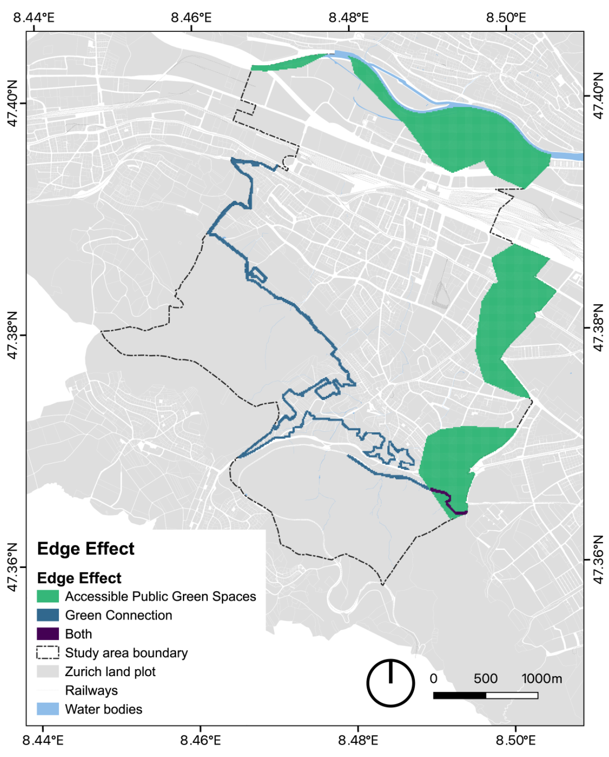
5.5. Geo-Boundary and Edge Effect

The research employed the administrative boundary of the Altstetten-Albisrieden district to generate grid cells and organise geo-information, resulting in edge effects in certain measurements of green factors (Figure 16). These effects arise from the geographic distribution or spatial occurrences within the district that may extend beyond its boundaries [82,83,84], particularly concerning green connections and the accessibility of public green spaces. In the analysis of the green connections, the predominant bias was identified in the cells adjacent to the western and southern boundaries, extending from the agricultural fields to the closed forest along the Uetliberg foothills, where the links to forests and fields were not incorporated. Certain public green spaces on the opposite riverbank of the Limmat are also accessible to residents in the northern part of the district; however, owing to the already elevated level of access to public green spaces in terms of both quantity and total area, this addition has minimal effects on the clustering results. City parks and gardens situated within 800 m to the east of the district may enhance the green attributes of the grid cells in the eastern part of the district regarding the availability of accessible public green spaces; nonetheless, in light of the contribution of each variable to the clusters, such impact may not be substantial.

The pressing concern regarding edge effects in the current study necessitates additional contemplation regarding boundary values and performance in the context of urban spatial phenomena. The continuous rise in the influx of individuals, transportation, and various materials has undermined traditional notions of boundaries, consequently complicating the comprehension of both local and global attributes. Defining a finite bounded area for spatial analysis may serve as a valuable supplementary aspect to this study.

6. Conclusions

From multiple perspectives, the importance of urban green infrastructure and its efficacy amid rapid urban development has received considerable attention. However, the existence of various configurations of urban green infrastructure, each offering distinct benefits, raises the question of how to enhance the provision of such infrastructure within existing urban environments, which is crucial for effective urban planning and design. This study aims to empirically investigate an integrated spatial analysis approach that synthesises the quality of urban green infrastructure and land characteristics by incorporating diverse perspectives, utilising the Altstetten-Albisrieden district of Zurich as a case study. The research conducted a systematic evaluation of the urban green infrastructure and employed grid-based analysis and clustering algorithms to generate spatial patterns indicative of unique land characteristics. This spatial analytical approach resulted in strategic recommendations for the Altstetten-Albisrieden district, informed by local land characteristics and incorporating a comprehensive understanding of the overall context at the district level.

The present condition of land use within the Altstetten-Albisrieden district exhibits a coherent spatial organisation characterised by an abundance of green spaces. This study categorises the district into five zones based on clustering results and the inherent characteristics of these clusters. It addresses the insufficiency of accessible public gardens and parks in the highly developed central regions while emphasising the critical need for community green spaces to offset the scarcity of expansive land designated for public open and green areas. The proposal of this study also includes utilising existing structures to enhance vegetation and plant life, particularly in zones adjacent to the industrial regions located centrally in the district. This approach aims to increase leaf area and improve connectivity between green patches and natural habitats in densely populated environments.

As an empirical study for integrating such spatial analysis, the metrics utilised can be further refined by enhancing data collection methods to mitigate edge effects, acquiring more precise information regarding ecosystems, and incorporating qualitative studies to substantiate accessibility and perceptions of public green spaces. The challenges posed by the high-dimensional dataset indicate a need for more sophisticated clustering methodologies to minimise randomness, thereby allowing the expansion of this approach to a broader scale. Regardless, this study establishes a robust foundation for understanding urban green infrastructure through the integration of multiple green factors based on their interrelations, thus encouraging future interdisciplinary urban and spatial research.

References

1. European Commission. Green Infrastructure. Environment. 2019. Available online: https://environment.ec.europa.eu/topics/nature-and-biodiversity/green-infrastructure_en#:~:text=Green%20infrastructure%20has%20been%20defined,example%2C%20water%20purification%2C%20improving%20air (accessed on 5 February 2025).
2. Hanna, E.; Comín, F.A. Urban Green Infrastructure and Sustainable Development: A Review. Sustainability 2021, 13, 11498. [Google Scholar] [CrossRef]
3. Wang, D.; Xu, P.-Y.; An, B.-W.; Guo, Q.-P. Urban green infrastructure: Bridging biodiversity conservation and sustainable urban development through adaptive management approach. Front. Ecol. Evol. 2024, 12, 1440477. [Google Scholar] [CrossRef]
4. Bowler, D.E.; Buyung-Ali, L.; Knight, T.M.; Pullin, A.S. Urban greening to cool towns and cities: A systematic review of the empirical evidence. Landsc. Urban Plan. 2010, 97, 147–155. [Google Scholar] [CrossRef]
5. Morabito, M.; Crisci, A.; Guerri, G.; Messeri, A.; Congedo, L.; Munafò, M. Surface urban heat islands in Italian metropolitan cities: Tree cover and impervious surface influences. Sci. Total Environ. 2021, 751, 142334. [Google Scholar] [CrossRef]
6. Xu, Z.; Rui, J. The mitigating effect of green Space’s spatial and temporal patterns on the urban heat island in the context of urban densification: A case study of Xi’an. Sustain. Cities Soc. 2024, 117, 105974. [Google Scholar] [CrossRef]
7. Lepczyk, C.A.; Aronson, M.F.J.; Evans, K.L.; Goddard, M.A.; Lerman, S.B.; MacIvor, J.S. Biodiversity in the City: Fundamental Questions for Understanding the Ecology of Urban Green Spaces for Biodiversity Conservation. BioScience 2017, 67, 799–807. [Google Scholar] [CrossRef]
8. Paudel, S.; States, S.L. Urban green spaces and sustainability: Exploring the ecosystem services and disservices of grassy lawns versus floral meadows. Urban For. Urban Green. 2023, 84, 127932. [Google Scholar] [CrossRef]
9. Jabbar, M.; Yusoff, M.M.; Shafie, A. Assessing the role of urban green spaces for human well-being: A systematic review. GeoJournal 2021, 87, 4405–4423. [Google Scholar] [CrossRef]
10. Wang’ombe, G. The Impact of Urban Green Spaces on Community Health and Well-being. Int. J. Arts Recreat. Sports 2024, 3, 14–25. [Google Scholar] [CrossRef]
11. Muluneh, M.G.; Worku, B.B. Contributions of urban green spaces for climate change mitigation and biodiversity conservation in Dessie city, Northeastern Ethiopia. Urban Clim. 2022, 46, 101294. [Google Scholar] [CrossRef]
12. Gill, S.E.; Handley, J.F.; Ennos, A.R.; Pauleit, S. Adapting Cities for Climate Change: The Role of the Green Infrastructure. Built Environ. 2007, 33, 115–133. [Google Scholar] [CrossRef]
13. Ai, K.; Yan, X. Can Green Infrastructure Investment Reduce Urban Carbon Emissions: Empirical Evidence from China. Land 2024, 13, 226. [Google Scholar] [CrossRef]
14. Liu, Y.; Han, B.; Jiang, C.Q.; Ouyang, Z. Uncovering the role of urban green infrastructure in carbon neutrality: A novel pathway from the urban green infrastructure and cooling power saving. J. Clean. Prod. 2024, 452, 142193. [Google Scholar] [CrossRef]
15. Deng, H.; Jim, C.Y. Spontaneous plant colonization and bird visits of tropical extensive green roof. Urban Ecosyst. 2017, 20, 337–352. [Google Scholar] [CrossRef]
16. Zhou, D.; Chu, L.M. How would size, age, human disturbance, and vegetation structure affect bird communities of urban parks in different seasons? J. Ornithol. 2012, 153, 1101–1112. [Google Scholar] [CrossRef]
17. Jiang, Y.; Menz, S.; Peric, A. Urban Greenery as a Tool to Enhance Social Integration? A Case Study of Altstetten-Albisrieden, Zürich. In Sustainable Built Environment; Yang, Y.-F., Ed.; IntechOpen: London, UK, 2023; Chapter 17. [Google Scholar] [CrossRef]
18. White, M.P.; Alcock, I.; Grellier, J.; Wheeler, B.W.; Hartig, T.; Warber, S.L.; Bone, A.; Depledge, M.H.; Fleming, L.E. Spending at least 120 min a week in nature is associated with good health and wellbeing. Sci. Rep. 2019, 9, 7730. [Google Scholar] [CrossRef]
19. Barboza, E.P.; Cirach, M.; Khomenko, S.; Iungman, T.; Mueller, N.; Barrera-Gómez, J.; Rojas-Rueda, D.; Kondo, M.; Nieuwenhuijsen, M. Green space and mortality in European cities: A health impact assessment study. Lancet Planet. Health 2021, 5, e718–e730. [Google Scholar] [CrossRef]
20. Cassin, J. History and development of nature-based solutions: Concepts and practice. In Nature-Based Solutions and Water Security; Elsevier: Amsterdam, The Netherlands, 2021; pp. 19–34. [Google Scholar] [CrossRef]
21. Cook, L.M.; Good, K.D.; Moretti, M.; Kremer, P.; Wadzuk, B.; Traver, R.; Smith, V. Towards the intentional multifunctionality of urban green infrastructure: A paradox of choice? npj Urban Sustain. 2024, 4, 12. [Google Scholar] [CrossRef]
22. Zhang, B.; MacKenzie, A. Trade-offs and synergies in urban green infrastructure: A systematic review. Urban For. Urban Green. 2024, 94, 128262. [Google Scholar] [CrossRef]
23. Abebe, M.T.; Megento, T.L. Urban green space development using GIS-based multi-criteria analysis in Addis Ababa metropolis. Appl. Geomat. 2017, 9, 247–261. [Google Scholar] [CrossRef]
24. Barton, D.N.; Dunford, R.; Gomez-Baggrthun, E.; Harrison, P.A.; Jacobs, S.; Kelemen, E.; Martin-Lopez, B. Integrated Assessment and Valuation of Ecosystem Services: Guidelines and Experiences (Collaborative Project FP7 Environment: OpenNESS. Operationalisation of Natural Capital and Ecosystem Services: From Concepts to Real-World Applications) [[Pu] After Publication of OpenNESS Special Issue in Ecosystem Services]. Finnish Environment Institute (SYKE). 2017. Available online: https://oppla.eu/sites/default/files/uploads/openness-d33-44integratedassessmentvaluationofesfinal2.pdf?utm_source=chatgpt.com (accessed on 5 February 2025).
25. Bousquet, M.; Kuller, M.; Lacroix, S.; Vanrolleghem, P.A. A critical review of multicriteria decision analysis practices in planning of urban green spaces and nature-based solutions. Blue-Green Syst. 2023, 5, 200–219. [Google Scholar] [CrossRef]
26. Gelan, E. GIS-based multi-criteria analysis for sustainable urban green spaces planning in emerging towns of Ethiopia: The case of Sululta town. Environ. Syst. Res. 2021, 10, 13. [Google Scholar] [CrossRef]
27. Langemeyer, J.; Gómez-Baggethun, E.; Haase, D.; Scheuer, S.; Elmqvist, T. Bridging the gap between ecosystem service assessments and land-use planning through Multi-Criteria Decision Analysis (MCDA). Environ. Sci. Policy 2016, 62, 45–56. [Google Scholar] [CrossRef]
28. Perić, A.; Jiang, Y.; Menz, S.; Ricci, L. Green Cities: Utopia or Reality? Evidence from Zurich, Switzerland. Sustainability 2023, 15, 12079. [Google Scholar] [CrossRef]
29. Chen, G.; Rong, L.; Zhang, G. Impacts of urban geometry on outdoor ventilation within idealized building arrays under unsteady diurnal cycles in summer. Build. Environ. 2021, 206, 108344. [Google Scholar] [CrossRef]
30. Hewitt, C.N.; Ashworth, K.; MacKenzie, A.R. Using green infrastructure to improve urban air quality (GI4AQ). Ambio 2020, 49, 62–73. [Google Scholar] [CrossRef]
31. Jin, M.-Y.; Apsunde, K.A.; Broderick, B.; Peng, Z.-R.; He, H.-D.; Gallagher, J. Evaluating the impact of evolving green and grey urban infrastructure on local particulate pollution around city square parks. Sci. Rep. 2024, 14, 18528. [Google Scholar] [CrossRef]
32. Dadvand, P.; Bartoll, X.; Basagaña, X.; Dalmau-Bueno, A.; Martinez, D.; Ambros, A.; Cirach, M.; Triguero-Mas, M.; Gascon, M.; Borrell, C.; et al. Green spaces and General Health: Roles of mental health status, social support, and physical activity. Environ. Int. 2016, 91, 161–167. [Google Scholar] [CrossRef]
33. Markevych, I.; Schoierer, J.; Hartig, T.; Chudnovsky, A.; Hystad, P.; Dzhambov, A.M.; De Vries, S.; Triguero-Mas, M.; Brauer, M.; Nieuwenhuijsen, M.J.; et al. Exploring pathways linking greenspace to health: Theoretical and methodological guidance. Environ. Res. 2017, 158, 301–317. [Google Scholar] [CrossRef]
34. van den Berg, A.E.; Maas, J.; Verheij, R.A.; Groenewegen, P.P. Green space as a buffer between stressful life events and health. Soc. Sci. Med. 2010, 70, 1203–1210. [Google Scholar] [CrossRef]
35. Zhang, F.; Qian, H. A comprehensive review of the environmental benefits of urban green spaces. Environ. Res. 2024, 252, 118837. [Google Scholar] [CrossRef] [PubMed]
36. Hartig, T.; Mitchell, R.; De Vries, S.; Frumkin, H. Nature and Health. Annu. Rev. Public Health 2014, 35, 207–228. [Google Scholar] [CrossRef] [PubMed]
37. Zhang, J.; Liu, Y.; Zhou, S.; Cheng, Y.; Zhao, B. Do various dimensions of exposure metrics affect biopsychosocial pathways linking green spaces to mental health? A cross-sectional study in Nanjing, China. Landsc. Urban Plan. 2022, 226, 104494. [Google Scholar] [CrossRef]
38. Bjerke, T.; Østdahl, T.; Thrane, C.; Strumse, E. Vegetation density of urban parks and perceived appropriateness for recreation. Urban For. Urban Green. 2006, 5, 35–44. [Google Scholar] [CrossRef]
39. Wang, M.; Qiu, M.; Chen, M.; Zhang, Y.; Zhang, S.; Wang, L. How does urban green space feature influence physical activity diversity in high-density built environment? An on-site observational study. Urban For. Urban Green. 2021, 62, 127129. [Google Scholar] [CrossRef]
40. Atlas. Grid-Based Analysis. Available online: https://atlas.co/glossary/grid-based-analysis/ (accessed on 10 December 2024).
41. Dong, N.; Yang, X.; Cai, H.; Xu, F. Research on Grid Size Suitability of Gridded Population Distribution in Urban Area: A Case Study in Urban Area of Xuanzhou District, China. PLoS ONE 2017, 12, e0170830. [Google Scholar] [CrossRef]
42. Kumari, A.; Geetha, P.; Shashank, A.; Rajendrakumar, S. Review on Grid-based system and applied GIS in Natural Resource management: A Comparative Analysis. Res. Sq. 2023, preprint. [Google Scholar] [CrossRef]
43. Luo, S.; Liu, Y.; Du, M.; Gao, S.; Wang, P.; Liu, X. The Influence of Spatial Grid Division on the Layout Analysis of Urban Functional Areas. ISPRS Int. J. Geo-Inf. 2021, 10, 189. [Google Scholar] [CrossRef]
44. Lv, H.; Wu, Z.; Guan, X.; Meng, Y.; Wang, H.; Zhou, Y. Threshold effect of data amount and grid size on urban land use type identification using multi-source data fusion. Sustain. Cities Soc. 2023, 98, 104855. [Google Scholar] [CrossRef]
45. Fang, H.; Baret, F.; Plummer, S.; Schaepman-Strub, G. An Overview of Global Leaf Area Index (LAI): Methods, Products, Validation, and Applications. Rev. Geophys. 2019, 57, 739–799. [Google Scholar] [CrossRef]
46. Chen, J.M.; Black, T.A. Defining leaf area index for non-flat leaves. Plant Cell Environ. 1992, 15, 421–429. [Google Scholar] [CrossRef]
47. Kang, Y.; Özdoğan, M.; Zipper, S.; Román, M.; Walker, J.; Hong, S.; Marshall, M.; Magliulo, V.; Moreno, J.; Alonso, L.; et al. How Universal Is the Relationship between Remotely Sensed Vegetation Indices and Crop Leaf Area Index? A Global Assessment. Remote Sens. 2016, 8, 597. [Google Scholar] [CrossRef] [PubMed]
48. Atzberger, C.; Darvishzadeh, R.; Immitzer, M.; Schlerf, M.; Skidmore, A.; Le Maire, G. Comparative analysis of different retrieval methods for mapping grassland leaf area index using airborne imaging spectroscopy. Int. J. Appl. Earth Obs. Geoinf. 2015, 43, 19–31. [Google Scholar] [CrossRef]
49. Swiss Federal Institute for Forest, Snow and Landscape Research. Insights into the Swiss Forest [Online Post]. 2011. Available online: https://www.lfi.ch/media/documents/publikationen/posterserie_LFI3_A4-en.pdf (accessed on 25 November 2024).
50. Thimonier, A.; Sedivy, I.; Schleppi, P. Estimating leaf area index in different types of mature forest stands in Switzerland: A comparison of methods. Eur. J. For. Res. 2010, 129, 543–562. [Google Scholar] [CrossRef]
51. Sterba, H.; Dirnberger, G.; Ritter, T. Vertical Distribution of Leaf Area of European Larch (Larix decidua Mill.) and Norway Spruce (Picea abies (L.) Karst.) in Pure and Mixed Stands. Forests 2019, 10, 570. [Google Scholar] [CrossRef]
52. Petritan, I.C.; Mihăilă, V.-V.; Bragă, C.I.; Boura, M.; Vasile, D.; Petritan, A.M. Litterfall production and leaf area index in a virgin European beech (Fagus sylvatica L.)—Silver fir (Abies alba Mill.) forest. Dendrobiology 2020, 83, 75–84. [Google Scholar] [CrossRef]
53. Chianucci, F.; Macfarlane, C.; Pisek, J.; Cutini, A.; Casa, R. Estimation of foliage clumping from the LAI-2000 Plant Canopy Analyzer: Effect of view caps. Trees 2015, 29, 355–366. [Google Scholar] [CrossRef]
54. Manetti, M.C.; Fabbio, G.; Giannini, T.; Gugliotta, O.I.; Gudi, G. Old-growth forests: Report from the plots established by Aldo Pavari. L’Italia For. E Mont. 2010, 65, 751–764. [Google Scholar] [CrossRef]
55. Montes, F.; Pita, P.; Rubio, A.; Cañellas, I. Leaf area index estimation in mountain even-aged Pinus silvestris L. stands from hemispherical photographs. Agric. For. Meteorol. 2007, 145, 215–228. [Google Scholar] [CrossRef]
56. Černý, J.; Haninec, P.; Pokorný, R. Leaf area index estimated by direct, semi-direct, and indirect methods in European beech and sycamore maple stands. J. For. Res. 2020, 31, 827–836. [Google Scholar] [CrossRef]
57. Ladefoged, K. Transpiration of Forest Trees in Closed Stands. Physiol. Plant. 1963, 16, 378–414. [Google Scholar] [CrossRef]
58. Šrámek, M.; Čermák, J. The vertical leaf distribution of Ulmus laevis Pall. Trees 2012, 26, 1781–1792. [Google Scholar] [CrossRef]
59. Nardini, A.; Raimondo, F.; Scimone, M.; Salleo, S. Impact of the leaf miner Cameraria ohridella on whole-plant photosynthetic productivity of Aesculus hippocastanum: Insights from a model. Trees 2004, 18, 714–721. [Google Scholar] [CrossRef]
60. Liu, Z.; Guo, P.; Liu, H.; Fan, P.; Zeng, P.; Liu, X.; Feng, C.; Wang, W.; Yang, F. Gradient Boosting Estimation of the Leaf Area Index of Apple Orchards in UAV Remote Sensing. Remote Sens. 2021, 13, 3263. [Google Scholar] [CrossRef]
61. Guo, X.; Yang, X.; Chen, M.; Li, M.; Wang, Y. A model with leaf area index and apple size parameters for 2.4 GHz radio propagation in apple orchards. Precis. Agric. 2015, 16, 180–200. [Google Scholar] [CrossRef]
62. Mora, M.; Avila, F.; Carrasco-Benavides, M.; Maldonado, G.; Olguín-Cáceres, J.; Fuentes, S. Automated computation of leaf area index from fruit trees using improved image processing algorithms applied to canopy cover digital photographies. Comput. Electron. Agric. 2016, 123, 195–202. [Google Scholar] [CrossRef]
63. Wei, S.; Wang, S.; Dong, R.; Dong, X. Indexes of Tree Structure of Cylindrical Pear Orchards at the Sapling Stage. Agric. Biotechnol. Cranston 2019, 8, 145–146. Available online: https://www.proquest.com/docview/2301479335?sourcetype=Scholarly%20Journals (accessed on 10 December 2024).
64. Peper, P.; McPherson, E.G. Comparison of Five Methods for Estimating Leaf Area Index of Open-Grown Deciduous Trees. Arboric. Urban For. 1998, 24, 98–111. [Google Scholar] [CrossRef]
65. Tokár, F. Aboveground biomass production in black walnut (Juglans nigra L.) Monocultures in dependence on leaf area index (lai) and climatic conditions. Ekologia 2009, 28, 234–241. [Google Scholar] [CrossRef]
66. Tharakan, P.J.; Volk, T.A.; Nowak, C.A.; Ofezu, G.J. Assessment of Canopy Structure, Light Interception, and Light-use Efficiency of First Year Regrowth of Shrub Willow (Salix sp.). BioEnergy Res. 2008, 1, 229–238. [Google Scholar] [CrossRef]
67. Parker, G.G. Tamm review: Leaf Area Index (LAI) is both a determinant and a consequence of important processes in vegetation canopies. For. Ecol. Manag. 2020, 477, 118496. [Google Scholar] [CrossRef]
68. Karaca, C.; Büyüktaş, D. Variation of The Leaf Area Index of Some Vegetables Commonly Grown in Greenhouse Conditions with Cultural Practices. Hortic. Stud. 2021, 38, 56–61. [Google Scholar] [CrossRef]
69. Nomura, K.; Ito, M.; Kusaba, Y.; Saito, M.; Mori, M.; Yamane, S.; Iwao, T.; Tada, I.; Yamazaki, T.; Kitano, M. Estimation of the optimal leaf area index (LAI) of an eggplant canopy based on the relationship between the nighttime respiration and daytime photosynthesis of the lowermost leaves. Sci. Hortic. 2023, 307, 111525. [Google Scholar] [CrossRef]
70. Mascarini, L.; Lorenzo, G.A.; Fernando, V. Leaf Area Index, Water Index, and Red: Far RedRatio Calculated by Spectral Reflectance and its Relation to Plant Architecture and Cut Rose Production. J. Am. Soc. Hortic. Sci. 2006, 131, 313–319. [Google Scholar]
71. Van Der Ploeg, A.; Heuvelink, E. The influence of temperature on growth and development of chrysanthemum cultivars. J. Hortic. Sci. Biotechnol. 2006, 81, 174–182. [Google Scholar] [CrossRef]
72. Rees, A.R. Dry-Matter Production by Field-Grown Tulips. J. Hortic. Sci. 1966, 41, 19–30. [Google Scholar] [CrossRef]
73. Dong, Y.; Li, G.; An, D.; Luo, W. Simulation model for predicting the effects of substrate water potential on leaf area of cut lily. Trans. Chin. Soc. Agric. Eng. (TCSAE) 2012, 28, 191–197. [Google Scholar]
74. Primack, R.B.; Morrison, R.A. Extinction, Causes of. In Encyclopaedia of Biodiversity; Elsevier: Amsterdam, The Netherlands, 2013; pp. 401–412. [Google Scholar] [CrossRef]
75. Diniz, M.F.; Cushman, S.A.; Machado, R.B.; De Marco Júnior, P. Landscape connectivity modeling from the perspective of animal dispersal. Landsc. Ecol. 2020, 35, 41–58. [Google Scholar] [CrossRef]
76. Parry-Thomson, R. Habitat fragmentation: Why It’s an Issue for Nature & Climate. Kent Wildlife Trust. 2024. Available online: https://www.kentwildlifetrust.org.uk/blog/habitat-fragmentation-impacts#:~:text=Habitat%20fragmentation%20occurs%20when%20larger,and%20the%20development%20of%20infrastructure (accessed on 7 December 2024).
77. Taylor, P.D.; Fahrig, L.; Henein, K.; Merriam, G. Connectivity Is a Vital Element of Landscape Structure. Oikos 1993, 68, 571. [Google Scholar] [CrossRef]
78. Zeller, K.A.; McGarigal, K.; Whiteley, A.R. Estimating landscape resistance to movement: A review. Landsc. Ecol. 2012, 27, 777–797. [Google Scholar] [CrossRef]
79. Brewer, C.A.; Pickle, L. Evaluation of Methods for Classifying Epidemiological Data on Choropleth Maps in Series. Ann. Assoc. Am. Geogr. 2002, 92, 662–681. [Google Scholar] [CrossRef]
80. von Luxburg, U. Clustering Stability: An Overview. arXiv 2010, arXiv:1007.1075. [Google Scholar] [CrossRef]
81. Rudnick, D.A.; Ryan, S.J.; Beier, P.; Cushman, S.A.; Dieffenbach, F.; Epps, C.W.; Gerber, L.R.; Hartter, J.; Jenness, J.S.; Kintsch, J.; et al. The role of landscape connectivity in planning and implementing conservation and restoration priorities. Ecology 2012, 16, 1–20. [Google Scholar]
82. Vidal Rodeiro, C.L.; Lawson, A.B. An evaluation of the edge effects in disease map modelling. Comput. Stat. Data Anal. 2005, 49, 45–62. [Google Scholar] [CrossRef]
83. Yamada, I. Edge Effects. In International Encyclopaedia of Human Geography; Elsevier: Amsterdam, The Netherlands, 2009; pp. 381–388. [Google Scholar] [CrossRef]
84. Gao, F.; Kihal, W.; Le Meur, N.; Souris, M.; Deguen, S. Does the edge effect impact on the measure of spatial accessibility to healthcare providers? Int. J. Health Geogr. 2017, 16, 46. [Google Scholar] [CrossRef]
Figure 1. Methodological framework of this study.
Land 14 00724 g001
Figure 2. Location of the studied district, Altstetten-Albisrieden, Zurich.
Land 14 00724 g002
Figure 3. Different grid sizes, 10-m grid (A) and 30-m grid (B), and their performance in reflecting the actual situation of building floor areas in the studied district.
Land 14 00724 g003
Figure 4. The concept of green connection calculation, counting the number of connections from one green patch to its neighbouring patches. The numbers in grid cells represent the number of connections.
Land 14 00724 g004
Figure 5. Development intensity (A), green surface (B), and leaf area (C) measured in a 10 m by 10 m rectangle grid across the studied area.
Land 14 00724 g005
Figure 6. Green ratio (A) and green connection (B) measured in a 10-m by 10-m rectangle grid across the studied area.
Land 14 00724 g006
Figure 7. The allocation of public green space throughout the studied district (A), the number of accessible public green spaces (B), and their total areas (C) within an 800-m walking distance in the district.
Land 14 00724 g007
Figure 8. Correlation coefficient analysis between seven measured factors (***: α = 0.001).
Land 14 00724 g008
Figure 9. Elbow Method and BIC analysing the optimal K value for the K-Means clustering algorithm: with all seven factors (A) and with four components retained after the PCA analysis (B). The red dash lines indicated a similar variation ratio from twenty clusters back and the elbow points as the optimal K values existed between ten and fifteen clusters.
Land 14 00724 g009
Figure 10. The PCA-reduced dimensional dataset projected in the three-dimensional system and clustered by different algorithms: 15 clusters by K-Means (A), 10 clusters by K-Means (B), 5 clusters by DBSCAN (C), 6 clusters by HDBSCAN (D), 15 clusters by GMM applying “VEV” model (E), and 9 clusters by the GMM applying the “VVE” model (F).
Land 14 00724 g010
Figure 11. Four clustering results projected into the studied district map: ten clusters by K-Means (A), fifteen clusters by K-Means (B), nine clusters through the “VVE” model in the GMM (C), and fifteen clusters through the “VEV” model in the GMM (D).
Land 14 00724 g011
Figure 12. Fifteen clusters by the K-Means clustering methods in the studied district and the seven-dimensional radar charts demonstrating the average characteristics of each cluster.
Land 14 00724 g012
Figure 13. Seven-dimensional characteristics of the five zones in the studied area. The colors of the radar charts were aligned with the distinct zone colors depicted in the accompanying map on the left side. The outlines were shaped by the overlapping radar charts of the encompassing clusters.
Land 14 00724 g013
Figure 14. Lindenplatz subsite in the studied district (A), its green clusters by K-Means clustering methods in a 10-m rectangle grid (B) and a 30-m rectangle grid (D), as well as the ten green clusters throughout the studied district within the 30-m rectangle grid (C).
Land 14 00724 g014
Figure 15. Contributions of each green factor to the clusters, with the colour varying from red to green indicating the contribution from high (level 5) to low (level 0).
Land 14 00724 g015
Figure 16. Edge effects in the studied areas highlight three possible impacts, as differentiated by the colours, when using administrative boundaries to limit the original data collection.
Land 14 00724 g016