Synergistic Evolution Characteristics and Driving Factors of High-Quality Economic Development and Green Space Ecological Benefits at Multiple Spatial Scales: Evidence from Shanxi Province, China

Abstract

Balancing economic growth with the decline in ecosystem service functions presents a critical global challenge in the 21st century. In response to the United Nations Development Programme’s emphasis on localizing Sustainable Development Goals, China has devised policies aimed at synergistically advancing high-quality economic development (HQED) and high-level ecological environment protection. However, research exploring the interplay between regional HQED and green space ecosystem services (GSES) remains limited. Consequently, this study examines Shanxi Province, a prototypical resource-based region in China, to develop localized metrics for green total factor productivity (GTFP) and the valuation of green space ecosystem services (GSESV). It quantifies the efficiency of HQED and the growth rate of green space ecological benefits (GSEB). Employing coupling coordination models, Theil indices, cluster analysis, and enhanced grey relational techniques, the research scrutinizes the evolutionary patterns and driving factors of coupling and coordination between HQED and GSEB across various spatial scales from 2007 to 2020. Significant findings include (1) an overall increase in HQED efficiency across all spatial scales, accompanied by a decline in green technological progress (GTC); (2) a sustained growth trend in GSEB per hectare across the province, with the southeastern region, particularly Jincheng, leading; (3) a level of coordination between HQED and GSEB across the province that surpasses the preliminary stage, albeit with pronounced regional disparities, notably the lagging and unstable coordination in the southern regions; (4) significant driving effects of industrial “three wastes” and industrial transformation on the coordinated evolution between HQED and GSEB across all spatial dimensions, with notable impacts of innovation input–output in central, southern, and southeastern Shanxi. This research offers new strategic insights for the synergistic development of the economy and ecology in Shanxi Province and contributes novel theoretical foundations for formulating sustainable development policies globally.

1. Introduction

Achieving regional sustainable development is a significant issue faced globally in the 21st century [1]. In 2015, the United Nations Sustainable Development Summit adopted “Transforming our World: The 2030 Agenda for Sustainable Development”, which proposed 17 Sustainable Development Goals (SDGs) and 169 sub-goals, and established a global evaluation mechanism framework for sustainable development [2]. In order to further respond to the call of the United Nations, in 2020, the Chinese government proposed at the 75th United Nations General Assembly to strive to reach the peak of carbon emissions by 2030 and achieve carbon neutrality by 2060 (referred to as the “dual carbon” goal) [3]. Under the “dual carbon” goal, how to balance economic growth and environmental protection became an urgent issue for the Chinese government. Since then, a series of policies to promote regional sustainable development have been promulgated in China. In 2021, China issued the “14th Five-Year Plan for National Economic and Social Development and the Outline of Long-Term Goals for 2035”, proposing to accelerate the green transformation of development methods, adhere to ecological priority and green development, and promote high-quality economic development and high-level protection of the ecological environment in a coordinated manner. In 2023, China issued the “Implementation Plan for Consolidating and Enhancing the Carbon Sequestration Capacity of Ecosystems”, proposing how to protect and restore ecosystems, enhance the carbon sequestration capacity of ecosystems, and respond to the challenges of global climate change. Therefore, analyzing the relationship between high-quality economic development (HQED) and ecosystem services (ES) is of significant importance. This analysis aids the Chinese government in implementing coordinated governance, thereby promoting sustainable regional development.

Scientific assessment of HQED is key to ensuring the achievement of the Sustainable Development Goals [4]. Given the diversity of national conditions, the United Nations Development Programme emphasizes the importance of localizing the Sustainable Development Goals. Therefore, regional assessment research on HQED is imperative. Total Factor Productivity (TFP) is an important indicator for measuring economic development efficiency [5]. As environmental issues are increasingly emphasized, scholars have incorporated environmental pollution variables into the calculation of TFP. The optimized TFP, which considers factors related to capital, labor, energy consumption, economic development, and environmental issues, is referred to as green total factor productivity (GTFP) [6]. It can more scientifically characterize the efficiency of HQED in the region [7,8]. Regarding the measurement of GTFP, some scholars use the DEA model [9], but this model does not consider the impact of random factors in the system. When there are outliers in the sample, the results of technical efficiency will be greatly affected. Most scholars use improved models of DEA, such as the SBM model [10] and the SDF model [11], but both models have radial defects. Some scholars use the Directional Distance Function (DDF) to calculate GTFP, which is a non-parametric method that overcomes the radial problem, but it cannot solve the problem of slack variables [12]. Tone and Tsutsui (2010) proposed a mixed distance function [13], the Epsilon-Based Measure (EBM) model. This model can overcome the defects of the SBM model and the DDF model by setting parameters, thereby improving the accuracy of GTFP measurement, and has been widely used in recent years [14,15]. Regarding the decomposition measurement of the GTFP index, the traditional method is to use the ML index for decomposition [12,14]. Since the ML index is the geometric mean of two current indices, there may be non-transitivity and linear programming solution defects in the decomposition process. Oh (2010) [16] proposed a GML index (Global Malmquist–Luenberger) decomposition method, which can overcome the defects of the ML index method and has been widely used in recent years [17,18].

It is undeniable that the secure supply of ES is the foundation for the sustainable growth of ecological benefits (EB) [19]. Therefore, sustainable development requires us to protect ecosystem services (ES) that are crucial to human livelihood and well-being while utilizing natural resources to ensure economic development and social functions [20]. However, the reality is that the contradiction between human activities and the natural environment is deepening, and a series of environmental problems have emerged, such as intensified land degradation [21], sharp reduction in biodiversity [22], imbalance in aquatic ecosystems [23], habitat fragmentation [24], deterioration of air quality [25], and intensified heat island effect [26], all of which signify the degradation of ecosystem service functions. The value of ecosystem services (ESV) refers to the various direct and indirect contributions provided by the ecosystem to humans, which are crucial to human well-being and quality of life [27]. The essence of ESV is to evaluate the quality of the human living environment and ecological production and to provide scientific support for ensuring sustainable socio-economic development [28], and it is an important indicator for measuring EB [29]. There are currently two widely used evaluation methods: the Ecological Modeling Method (EMM) [30] and the Equivalent Factor Method (EFM) [31]. EMM includes a series of ecological functions, requires multiple data sources, and involves various complex equations [32]. EFM is based on “equivalent values” (average value per unit area) and corresponding areas and is suitable for large-scale aggregation of the value of multiple services [33].

Green spaces (GS), as integral components of ecosystems, possess significant ESV [34,35]. The synergistic evolution between HQED and the ecological benefits of green spaces (GSEB) directly influences the interaction between human society and the natural environment. If there is a high degree of consistency and coordination between the HQED and the GSEB, it implies that economic development can continue without damaging the ecological environment. Coordinated development characterizes the orderly state of benign interaction and harmony among various elements within the system evolution process and can effectively reflect the overall level of element development and their synergistic effects [36]. The coupling coordination model is a mathematical model used to assess the interaction and coordination between two or more systems. The core of this model lies in quantifying the degree of coupling between systems and their coordination in operation [37]. At present, many scholars use the coupling coordination model to explore the relationship between ecosystems and human development [38,39,40], providing a reference for conducting research on the coordination between HQED and GSEB. In addition, it is equally important to reveal the driving mechanism of the coordinated evolution between HQED and the GSEB. This provides a reference for formulating future development policies and determining current management needs. Current methods used to explore the degree of influence of driving factors mainly include correlation analysis [41], obstacle degree model [42], principal component analysis [43], regression analysis [44], and grey correlation analysis [45]. Therefore, it is necessary to use these mathematical methods to measure the correlation between driving factors and coordination in order to reveal their specific association types.

Current research on the relationship between HQED and GSEB remains limited. Shanxi Province, a typical resource-based region, is characterized by severe resource depletion and an extremely fragile ecosystem. The deterioration of the environment, in turn, constrains the region’s HQED, posing significant challenges to sustainable development [46]. Against this backdrop, this study proposes the following innovations. (1) In consideration of China’s “dual carbon” goals and data availability, we have constructed a localized GTFP assessment framework and applied it to quantitatively evaluate the efficiency of HQED in Shanxi Province. Additionally, based on the production and price data of Shanxi’s major crops, we have developed a localized GSESV evaluation system, which has been employed to quantitatively assess the growth rate of GSEB. (2) By integrating various mathematical models, we conducted a coupled coordination analysis of HQED efficiency and the growth rate of GSEB across different spatial scales, providing an in-depth exploration of the evolutionary relationship between the two. (3) Utilizing an improved grey relational analysis model, we quantified the driving forces of different factors on the coordinated development across various spatial scale levels, thereby offering a foundation for policymakers at different administrative levels to formulate sustainable development strategies. Through this study, we aim to promote the sustainable development of the regional economy and environment, fostering harmonious coexistence between humanity and nature.

2. Materials and Methods

2.1. Study Area

Shanxi Province is situated between 34°34′ and 40°44′ N latitude and 110°14′ and 114°33′ E longitude. The region is characterized by a temperate continental monsoon climate and features highly diverse topographical conditions. It spans the Yellow River and Haihe River basins, serving as a transitional zone between the North China Plain and the Loess Plateau. The complex terrain, marked by interwoven valleys, has led to severe soil erosion (Figure 1a–c). As one of China’s key ecologically fragile areas, Shanxi Province faces significant environmental challenges [47,48]. As of the end of 2023, Shanxi Province has jurisdiction over 11 prefecture-level cities, divided into four major regions: north, central, south, and southeast (Figure 1d). It is worth noting that Shanxi Province, as one of China’s major coal production bases, is facing problems such as ecological environmental degradation [49] and industrial structure imbalance [50,51] due to long-term coal mining and reliance on a coal-dominated industrial structure. In response to these problems, the Shanxi provincial government has taken measures for ecological restoration and transformation and upgrading, including the development of clean energy, promotion of clean and efficient use of coal, strengthening of environmental protection and pollution control, and restoration of green space ecosystems [52,53]. Conducting research on the coupling characteristics of HQED and GSEB in this region can not only verify the positive results of the policies implemented by the government but also provide direction for the formulation of future development policies in the region, which is conducive to promoting the sustainable development of society and the construction of ecological civilization.

2.2. Data Source and Processing

The timeframe of the original data utilized in this study is divided into two components. (1) The calculation of the growth rates of high-quality economic development (HQED) and green space ecological benefits (GSEB) for the years 2007–2020 requires original data from the preceding year as the computational basis. Consequently, the relevant original data span the years 2006–2020. (2) Data pertaining to the driving mechanisms of coordinated development are exclusively focused on the period 2007–2020.

The sources of the original data are detailed as follows.

(1)

The land use data spans from 2006 to 2020, sourced from the Annual China Land Cover Dataset (CLCD). The land use types in CLCD include farmland, forest, shrub, grassland, water area, bare land, and impervious surface, with a spatial resolution of 30 M, and it provides continuous annual data [54]. This study refers to existing research results [55,56] and the “Classification of Current Land Use Status” (GB/T21010-2017) issued by the Ministry of Natural Resources of China to classify land use in Shanxi Province (see

Table 1. Classification of land use types.

First-Level Classification	Second-Level Classification	Spatial Type Meaning	Data Source
Green Space	Farmland	Land used for crop cultivation.	Annual China Land Cover Dataset (CLCD); (https://zenodo.org/records/8176941 (accessed on 6 October 2024))
	Woodland	Refers to land predominantly covered by forest vegetation, including both natural and artificial forests. The vegetation in forested areas typically comprises trees (tall woody plants), shrubs, and various types of understory vegetation.
	Grassland	Land well covered by herbaceous plants.
	Water Area	All water spaces.
Non-Green Space	Bare Land	Land containing bare soil and bare rocky gravel.
	Impervious Surface	The primary components include buildings, roads, squares, parking lots, and other hard surfaces, as well as land covered with artificial materials and urban construction areas.

for details).

(2)

The annual grain price data spans from 2006 to 2020, sourced from the “National Compilation of Agricultural Product Cost and Income Data”. The primary data collected pertain to the grain yield per unit area and grain prices in Shanxi Province (refer to Table 2 for details).

(3)

The HQED is characterized by GTFP. The original data, ranging from 2006 to 2020, are primarily derived from the “Shanxi Provincial Statistical Yearbook”, “China Urban Statistical Yearbook”, China Carbon Accounting Database, and statistical bulletins of 11 prefecture-level cities (refer to Table 2 for details).

(4)

The original data for the driving factors, spanning from 2007 to 2020, are entirely sourced from the “China Urban Statistical Yearbook”.

2.3. Research Methodology

This study primarily encompasses four sections. (1) Based on the raw data from 2006 to 2020, this study calculates the efficiency of high-quality economic development (HQED) in Shanxi Province across different spatial scales for the period 2007–2020, represented by green total factor productivity, and systematically analyzes its evolutionary characteristics. (2) Using land use data from 2006 to 2020, the ecological benefits of green spaces (GSEB) in Shanxi Province across various spatial scales are computed for 2006–2020, along with the ecological benefit growth rates for 2007–2020, forming the basis for analyzing their evolutionary trends. (3) The coupling coordination degree between HQED and GSEB is calculated for 2007–2020, and their synergistic evolutionary trends are analyzed in detail. (4) An improved grey relational analysis method is employed to examine the driving mechanisms behind the coordinated development of HQED and GSEB. The detailed content is illustrated in Figure 2.

2.3.1. Efficiency of High-Quality Economic Development

(1)

Construction of Evaluation Index System

This paper primarily characterizes the efficiency of HQED through GTFP. Referring to existing literature [57,58,59,60,61], and in conjunction with the “dual carbon” goals and the actual situation in Shanxi Province, GTFP evaluation indicators are selected from three aspects: input, expected output, and non-expected output. Further, each indicator undergoes correlation analysis, with the calculation formula for the correlation coefficient detailed in the literature [62]. The Variance Inflation Factor (VIF) method is utilized to eliminate some indicators with high correlation. The calculation formula is as follows:

$$\mathrm{V}\mathrm{I}\mathrm{F}={\displaystyle \frac{1}{1-{\mathrm{R}}^2}}$$

(1)

In the formula, R represents the correlation coefficient among all indicators contained in each driving factor. Generally, when the VIF is greater than 10 (i.e., VIF > 10), and consequently R² > 0.9, it is considered that there is multicollinearity among the indicators. Conversely, when the VIF is between 0 and 10 (i.e., 0 ≤ VIF ≤ 10), it is considered that there is no collinearity among the indicators.

We eliminate indicators with a VIF greater than 10 (VIF > 10) and ultimately construct the evaluation index system for GTFP. The weights of each indicator are calculated using the entropy weight method [63]. The detailed weights of each indicator are presented in Table 2.

Table 2. Evaluation Index System for GTFP.

	First-Level Indicator	Second-Level Indicator	Weight	Indicator Description	Data Time	Data Source
GTFP	Inputs	Number of persons employed (10,000 people)	0.1191	Province and 11 cities	2006–2020	“Shanxi Statistical Yearbook” and “China City Statistical Yearbook”, 2007–2021.
		Urban built-up area (km2)	0.0966	Province and 11 cities	2006–2020	“Shanxi Statistical Yearbook” and “China City Statistical Yearbook”, 2007–2021.
		Capital stock (USD million)	0.0521	2006 base year. Province and 11 cities	2006–2020	“Shanxi Statistical Yearbook” and “China City Statistical Yearbook”, 2007–2021. The calculation formula for capital stock refers to Amini Parsa et al., 2019 [64].
		Energy consumption (tons of standard coal)	0.0405	Province and 11 cities	2006–2020	“Shanxi Provincial Statistical Yearbook”, 2007–2021; Statistical bulletins of 11 prefecture-level cities, 2007–2021.
	Desirable outputs	GDP (USD million)	0.1662	2006 base year reduction. Province and 11 cities	2006–2020	“Shanxi Statistical Yearbook”, 2007–2021.
	Undesirable outputs	Industrial SO2 emissions(tons)	0.0541	Province and 11 cities	2006–2020	“Shanxi Statistical Yearbook” and “China City Statistical Yearbook”, 2007–2021.
		Industrial wastewater discharge (tons)	0.0574	Province and 11 cities	2006–2020	“Shanxi Statistical Yearbook” and “China City Statistical Yearbook”, 2007–2021.
		Cumulative area of land damaged by mining (hm2)	0.1623	Province and 11 cities	2006–2020	Shanxi Provincial Department of Natural Resources.
		CO2 emission (tons)	0.2518	Province and 11 cities	2006–2020	The data comes from the China Carbon Accounting Database (https://www.ceads.net/user/login.php?lang=cn (accessed on 6 October 2024)).

Note: The statistical yearbook published in the year T + 1 actually contains data for the year T. Therefore, the data for 2006–2020 are derived from the statistical yearbooks of 2007–2021.

Table 2. Evaluation Index System for GTFP.

	First-Level Indicator	Second-Level Indicator	Weight	Indicator Description	Data Time	Data Source
GTFP	Inputs	Number of persons employed (10,000 people)	0.1191	Province and 11 cities	2006–2020	“Shanxi Statistical Yearbook” and “China City Statistical Yearbook”, 2007–2021.
		Urban built-up area (km2)	0.0966	Province and 11 cities	2006–2020	“Shanxi Statistical Yearbook” and “China City Statistical Yearbook”, 2007–2021.
		Capital stock (USD million)	0.0521	2006 base year. Province and 11 cities	2006–2020	“Shanxi Statistical Yearbook” and “China City Statistical Yearbook”, 2007–2021. The calculation formula for capital stock refers to Amini Parsa et al., 2019 [64].
		Energy consumption (tons of standard coal)	0.0405	Province and 11 cities	2006–2020	“Shanxi Provincial Statistical Yearbook”, 2007–2021; Statistical bulletins of 11 prefecture-level cities, 2007–2021.
	Desirable outputs	GDP (USD million)	0.1662	2006 base year reduction. Province and 11 cities	2006–2020	“Shanxi Statistical Yearbook”, 2007–2021.
	Undesirable outputs	Industrial SO2 emissions(tons)	0.0541	Province and 11 cities	2006–2020	“Shanxi Statistical Yearbook” and “China City Statistical Yearbook”, 2007–2021.
		Industrial wastewater discharge (tons)	0.0574	Province and 11 cities	2006–2020	“Shanxi Statistical Yearbook” and “China City Statistical Yearbook”, 2007–2021.
		Cumulative area of land damaged by mining (hm2)	0.1623	Province and 11 cities	2006–2020	Shanxi Provincial Department of Natural Resources.
		CO2 emission (tons)	0.2518	Province and 11 cities	2006–2020	The data comes from the China Carbon Accounting Database (https://www.ceads.net/user/login.php?lang=cn (accessed on 6 October 2024)).

Note: The statistical yearbook published in the year T + 1 actually contains data for the year T. Therefore, the data for 2006–2020 are derived from the statistical yearbooks of 2007–2021.

(2)

Calculating GTFP Using the EBM Model

The construction of the EBM model is as follows.

Assume there are K decision units; each decision unit includes M types of inputs, N types of expected outputs, and L types of waste outputs. The formula is as follows:

$$\gamma =\mathrm{m}\mathrm{i}\mathrm{n}{\displaystyle \frac{\theta -{\epsilon }_{\mathrm{x}}\sum _{\mathrm{i}=1}^{\mathrm{m}}\frac{{\omega }_{\mathrm{i}}^{-}{\mathrm{s}}_{\mathrm{i}}^{-}}{{\mathrm{x}}_{\mathrm{i}\mathrm{k}}}}{\phi +{\epsilon }_{\mathrm{y}}\sum _{\mathrm{j}=1}^{\mathrm{n}}\frac{{\omega }_{\mathrm{j}}^{+}{\mathrm{s}}_{\mathrm{j}}^{+}}{{\mathrm{y}}_{\mathrm{j}\mathrm{k}}}+{\epsilon }_{\mathrm{b}}\sum _{\mathrm{z}=1}^{\mathrm{t}}\frac{{\omega }_{\mathrm{z}}^{-}{\mathrm{s}}_{\mathrm{z}}^{-}}{{\mathrm{b}}_{\mathrm{z}\mathrm{k}}}}}$$

(2)

$$\mathrm{s}.\mathrm{t}.\mathrm{X}\delta +{\mathrm{S}}_{\mathrm{i}}^{-}=\theta {\mathrm{x}}_{\mathrm{k}},\mathrm{i}=1,2,\dots ,\mathrm{m}$$

(3)

$$\mathrm{Y}\delta -{\mathrm{s}}_{\mathrm{j}}^{+}=\phi {\mathrm{y}}_{\mathrm{k}},\mathrm{j}=1,2,\dots ,\mathrm{n}$$

(4)

$$\mathrm{B}\delta +{\mathrm{s}}_{\mathrm{z}}^{-}=\phi {\mathrm{b}}_{\mathrm{k}},\mathrm{z}=1,2,\dots ,\mathrm{l}$$

(5)

$$\delta \ge 0,{\mathrm{s}}_{\mathrm{i}}^{-},{\mathrm{s}}_{\mathrm{j}}^{+},{\mathrm{s}}_{\mathrm{z}}^{-}\ge 0$$

Herein, γ is the optimal efficiency value, satisfying 0 ≤ $\gamma$ ≤ 1. ${\omega }_{\mathrm{i}}^{-}$ and ${\mathrm{s}}_{\mathrm{i}}^{-},$ respectively, represent the weight and slack of the ith input indicator; ${\omega }_{\mathrm{j}}^{+}$ and ${\mathrm{s}}_{\mathrm{j}}^{+},$ respectively, represent the weight and slack of the j-th expected output indicator; ${\omega }_{\mathrm{z}}^{-}$ and ${\mathrm{s}}_{\mathrm{z}}^{-}$ represent the weight and slack of the z-th unexpected output indicator. $\epsilon$ is the core parameter of the EBM, which is an important indicator of the comprehensive radial efficiency value θ and the non-radial slack variable. The value range of $\epsilon$ is [0, 1]. When $\epsilon$ = 0, it is equivalent to the radial CCR model. When $\epsilon$ = 1, it is equivalent to the SBM model. When $\epsilon$ is between 0 and 1, it indicates that the model contains both radial and non-radial slack variable parts.

(3)

Decomposing GTFP Using the GML Index

Based on the calculation of the green total factor productivity from 2007 to 2020, this paper further decomposes it to obtain the technological progress index and efficiency improvement index from 2007 to 2020. This paper draws on the decomposition ideas of Oh (2010) [16] and introduces the GML index (Global Malmquist–Luenberger) decomposition method. The GML index method constructs a global production possibility set. The specific formula is as follows:

$${\mathrm{G}\mathrm{M}\mathrm{L}}^{\mathrm{T},\mathrm{T}+1}\left({\mathrm{x}}^{\mathrm{T}},{\mathrm{y}}^{\mathrm{T}},{\mathrm{b}}^{\mathrm{T}},{\mathrm{x}}^{\mathrm{T}+1},{\mathrm{y}}^{\mathrm{T}+1},{\mathrm{b}}^{\mathrm{T}+1}\right)={\displaystyle \frac{{\mathrm{E}}^{\mathrm{G},\mathrm{T}+1}\left({\mathrm{x}}^{\mathrm{T}+1},{\mathrm{y}}^{\mathrm{T}+1},{\mathrm{b}}^{\mathrm{T}+1}\right)}{{\mathrm{E}}^{\mathrm{G},\mathrm{T}}\left({\mathrm{x}}^{\mathrm{T}},{\mathrm{y}}^{\mathrm{T}},{\mathrm{b}}^{\mathrm{T}}\right)}}=$$

$${\displaystyle \frac{{\mathrm{E}}^{\mathrm{T}+1}\left({\mathrm{x}}^{\mathrm{T}+1},{\mathrm{y}}^{\mathrm{T}+1},{\mathrm{b}}^{\mathrm{T}+1}\right)}{{\mathrm{E}}^{\mathrm{T}}\left({\mathrm{x}}^{\mathrm{T}},{\mathrm{y}}^{\mathrm{T}},{\mathrm{b}}^{\mathrm{T}}\right)}}\ast {\displaystyle \frac{\raisebox{1ex}{${\mathrm{E}}^{\mathrm{G},\mathrm{T}+1}\left({\mathrm{x}}^{\mathrm{T}+1},{\mathrm{y}}^{\mathrm{T}+1},{\mathrm{b}}^{\mathrm{T}+1}\right)$}\!\left/ \!\raisebox{-1ex}{${\mathrm{E}}^{\mathrm{T}+1}\left({\mathrm{x}}^{\mathrm{T}+1},{\mathrm{y}}^{\mathrm{T}+1},{\mathrm{b}}^{\mathrm{T}+1}\right)$}\right.}{\raisebox{1ex}{${\mathrm{E}}^{\mathrm{G},\mathrm{T}}\left({\mathrm{x}}^{\mathrm{T}},{\mathrm{y}}^{\mathrm{T}},{\mathrm{b}}^{\mathrm{T}}\right)$}\!\left/ \!\raisebox{-1ex}{${\mathrm{E}}^{\mathrm{T}}\left({\mathrm{x}}^{\mathrm{T}},{\mathrm{y}}^{\mathrm{T}},{\mathrm{b}}^{\mathrm{T}}\right)$}\right.}}={\mathrm{G}\mathrm{M}\mathrm{L}\mathrm{E}\mathrm{C}}^{\mathrm{T},\mathrm{T}+1}\ast {\mathrm{G}\mathrm{M}\mathrm{L}\mathrm{T}\mathrm{C}}^{\mathrm{T},\mathrm{T}+1}$$

(6)

Herein, E (G, T + 1) represents the global efficiency value in year T + 1. GML stands for the GTFP, which can be decomposed into GMLEC and GMLTC, i.e., green efficiency change (GEC) and green technical change (GTC). Generally, GEC reflects the improvement of management efficiency, the rise of labor proficiency, etc., while GTC is an important indicator to measure the real level of technology. When GTC > 1, it represents green technological progress; when GTC < 1, it represents green technological regression; when GTC = 1, it indicates that the level of green technology remains unchanged. When GEC > 1, it represents green efficiency progress; when GEC < 1, it represents green efficiency regression; when GEC = 1, it indicates that the level of green efficiency remains unchanged.

2.3.2. Measurement of Green Space Ecological Benefits

This study employs ecosystem service value (ESV) as a representation of ecological benefits (EB). The evaluation framework for green space ecological benefits (GSEB) is constructed using the equivalent factor method proposed by Xie et al. (2008) [65]. This framework encompasses four dimensions: provisioning services, regulating services, supporting services, and cultural services. The equivalent factors derived by Xie et al. (2010) [66] represent the average service value of China’s ecosystems. Given the regional differences, this study applies the revision method proposed by Liu et al. (2020) [67] to adjust the temporal and spatial components of the existing calculations. The spatial component uses the ratio of the grain yield per unit area in the research area to that of China’s arable land as a correction coefficient, adjusting the ecosystem service value per unit area to match that of Shanxi Province. The temporal component uses the average grain yield data per unit area from 2006 to 2020 to correct the service value per unit area in Shanxi Province. To mitigate the impact of inflation, the average prices of the main crops (wheat and corn) in Shanxi Province from 2006 to 2020 (0.31 USD/kg) are used as the base data, with the annual average yield of wheat and corn from 2006 to 2020 (3209.83 kg/hm²) serving as the benchmark yield. Existing research indicates that the economic value provided by the natural ecosystem without human capital input is 1/7 of the economic value of food production services provided by the existing unit area of farmland [68]. Based on this, the equivalent value per hectare of various types of green space ecosystem services in Shanxi Province and the weights of each indicator (

Table 3. ESV equivalents per hectare for various types of green space.

	First-Level Indicator	Second-Level Indicator	Weight	Farmland /USD·hm−2	Woodland /USD·hm−2	Grassland /USD·hm−2	Water Area /USD·hm−2
ESV	Provisioning Services	Food Production	0.020453	160.98	53.10	69.20	85.24
		Raw Material Production	0.036444	62.77	479.73	57.89	56.23
		Water Resource Supply	0.157507	3.07	248.16	32.09	2554.55
	Regulating Services	Gas Regulation	0.062978	115.78	695.39	241.50	82.04
		Climate Regulation	0.077366	156.10	655.08	251.13	331.63
		Waste Regulation	0.172271	223.75	276.76	212.48	2390.90
		Hydrological Regulation	0.224731	123.87	658.43	244.71	3022.07
	Supporting Services	Soil Conservation	0.072732	236.59	647.22	360.65	65.99
		Maintain Nutrient Cycle	0.011204	18.83	146.77	19.11	17.16
		Maintain Biodiversity	0.096769	164.19	726.05	301.08	552.21
	Cultural Services	Provide Aesthetic Landscape	0.067545	27.34	334.84	140.07	714.74
	Total		1	1293.27	4921.87	1968.02	9872.76

Note: The values in the table were converted based on the exchange rate between USD and CNY on 1 August 2023.

) are determined. Upon examining different ecosystem functions, it is found that the EB of water areas and woodlands is higher. Among the first-level indicators, regulation services carry the highest weight, while cultural services have the lowest. The top three weights among the second-level indicators are hydrological regulation, waste regulation, and water resource supply, with the lowest weight indicator being nutrient cycling maintenance.

Based on the land area of each type of green space from 2006 to 2020, the study calculates the ecological benefits per hectare of green space (GSEB) across different spatial scales. The formula is as follows:

$$\mathrm{G}\mathrm{S}\mathrm{E}\mathrm{B}={\displaystyle \frac{\sum _{\mathrm{i}=1}^4{\mathrm{S}}_{\mathrm{i}}\times \mathrm{V}{\mathrm{C}}_{\mathrm{i}}}{\mathrm{S}}}$$

(7)

Here, GSEB is the total ESV per hectare of green space, S_i is the area of the ith type of land use in the research area, VC_i is the ESV per unit area of the ith type of land use, and S represents the total area of different spatial scales.

This study utilizes the year-on-year growth rate of green space ecological benefits (GSEB) from 2007 to 2020 to represent the annual variation in ecological benefits. The formula is as follows:

$${\mathrm{G}}_{\mathrm{T}}={\displaystyle \frac{{\mathrm{G}\mathrm{S}\mathrm{E}\mathrm{B}}_{\mathrm{T}}-{\mathrm{G}\mathrm{S}\mathrm{E}\mathrm{B}}_{\mathrm{T}-1}}{{\mathrm{G}\mathrm{S}\mathrm{E}\mathrm{B}}_{\mathrm{T}-1}}}\times 100\mathrm{\%},\mathrm{T}=2007,2008,\dots ,2020$$

(8)

Here, ${\mathrm{G}}_{\mathrm{T}}$ represents the growth rate of GSEB in the T year compared to the (T − 1) year, GSEB_T−1 and GSEB_T, respectively, represent the GSEB of the (T − 1) year and the T year. When G_T > 0, it means that GSEB has increased compared to the previous year; when G_T = 0, it means that GSEB remains unchanged; when G_T <0, it means that GSEB has decreased compared to the previous year.

2.3.3. Coupling Coordination Degree Calculation

(1)

Data Standardization

Before calculating the coupling coordination degree, the GTFP, GTC, GEC, and G_T data from 2007 to 2020 at various spatial scales are standardized. The specific formula is as follows:

$$\mu ={\displaystyle \frac{\mathrm{z}-{\mathrm{z}}_{\mathrm{m}\mathrm{i}\mathrm{n}}}{{\mathrm{z}}_{\mathrm{m}\mathrm{a}\mathrm{x}}-{\mathrm{z}}_{\mathrm{m}\mathrm{i}\mathrm{n}}}}$$

(9)

Here, z is the original value; z_max is the maximum value of the data set; z_min is the minimum value of the data set; μ is the transformed value.

(2)

Calculation of Coupling Coordination Degree

The formula for the coupling coordination degree model is:

$$\mathrm{Y}=\sqrt{{2[{\displaystyle \frac{{\mu }_1\times {\mu }_2}{{\left({\mu }_{1+}{\mu }_2\right)}^2}}]}^{{\displaystyle \raisebox{1ex}{$1$}\!\left/ \!\raisebox{-1ex}{$2$}\right.}}\times (\alpha {\mu }_1+\beta {\mu }_2)}$$

(10)

Here, ${\mu }_1$ is GTFP or GTC or GEC after standardization, ${\mu }_2$ is the standardized G_T; α, β are the coefficients to be determined, reflecting the relative importance of the two systems. This paper believes that HQED and GSEB play equally important roles, so α = 0.5, β = 0.5. The coordination degree is divided into 9 levels and then combined with the relative size of ${\mu }_1$ and ${\mu }_2$, the relative synchronization degree of HQED and GSEB is determined. The coordination relationship between GTFP, GTC, GEC, and G_T is represented by GTFP-G_T, GTC-G_T, GEC-G_T, respectively, and the specific classification is shown in

Table A1. Classification of Coordination Degree of High-Quality Economic Development and Green Space Ecological Benefits.

Type	Coordination Level	Coordination Development Threshold	Synchronization Level	Synchronization Classification	Relationship Judgment
					$\mathbf{G}\mathbf{T}\mathbf{F}\mathbf{P}-{\mathit{G}}_{\mathit{T}}$	$\mathbf{G}\mathbf{T}\mathbf{C}-{\mathit{G}}_{\mathit{T}}$	$\mathbf{G}\mathbf{E}\mathbf{C}-{\mathit{G}}_{\mathit{T}}$
High-quality Coordination	I	$0.9<Y\le 1$	A	$|{\mu }_1-{\mu }_2|\le 0.1$	High-quality Coordination − Synchronization	High-quality Coordination − Synchronization	High-quality Coordination − Synchronization
			B	${\mu }_1-{\mu }_2>0.1$	High-quality Coordination − GSEB Lagging	High-quality Coordination − GSEB Lagging	High-quality Coordination − GSEB Lagging
			C	${\mu }_2-{\mu }_1>0.1$	High-quality Coordination − GTFP Lagging	High-quality Coordination − GTC Lagging	High-quality Coordination − GEC Lagging
Good Coordination	II	$0.8<Y\le 0.9$	A	$|{\mu }_1-{\mu }_2|\le 0.1$	Good Coordination − Synchronization	Good Coordination − Synchronization	Good Coordination − Synchronization
			B	${\mu }_1-{\mu }_2>0.1$	Good Coordination − GSEB Lagging	Good Coordination − GSEB Lagging	Good Coordination − GSEB Lagging
			C	${\mu }_2-{\mu }_1>0.1$	Good Coordination − GTFP Lagging	Good Coordination − GTC Lagging	Good Coordination − GEC Lagging
Intermediate Coordination	III	$0.7<Y\le 0.8$	A	$|{\mu }_1-{\mu }_2|\le 0.1$	Intermediate Coordination − Synchronization	Intermediate Coordination − Synchronization	Intermediate Coordination − Synchronization
			B	${\mu }_1-{\mu }_2>0.1$	Intermediate Coordination − GSEB Lagging	Intermediate Coordination − GSEB Lagging	Intermediate Coordination − GSEB Lagging
			C	${\mu }_2-{\mu }_1>0.1$	Intermediate Coordination − GTFP Lagging	Intermediate Coordination − GTC Lagging	Intermediate Coordination − GEC Lagging
Primary Coordination	IV	$0.6<Y\le 0.7$	A	$|{\mu }_1-{\mu }_2|\le 0.1$	Primary Coordination − Synchronization	Primary Coordination − Synchronization	Primary Coordination − Synchronization
			B	${\mu }_1-{\mu }_2>0.1$	Primary Coordination − GSEB Lagging	Primary Coordination − GSEB Lagging	Primary Coordination − GSEB Lagging
			C	${\mu }_2-{\mu }_1>0.1$	Primary Coordination − GTFP Lagging	Primary Coordination − GTC Lagging	Primary Coordination − GEC Lagging
On the Verge of Discord	V	$0.5<Y\le 0.6$	A	$|{\mu }_1-{\mu }_2|\le 0.1$	On the Verge of Discord − Synchronization	On the Verge of Discord − Synchronization	On the Verge of Discord − Synchronization
			B	${\mu }_1-{\mu }_2>0.1$	On the Verge of Discord − GSEB Lagging	On the Verge of Discord − GSEB Lagging	On the Verge of Discord − GSEB Lagging
			C	${\mu }_2-{\mu }_1>0.1$	On the Verge of Discord − GTFP Lagging	On the Verge of Discord − GTC Lagging	On the Verge of Discord − GEC Lagging
Mild Discord	VI	$0.4<Y\le 0.5$	A	$|{\mu }_1-{\mu }_2|\le 0.1$	Mild Discord − Synchronization	Mild Discord − Synchronization	Mild Discord − Synchronization
			B	${\mu }_1-{\mu }_2>0.1$	Mild Discord − GSEB Lagging	Mild Discord − GSEB Lagging	Mild Discord − GSEB Lagging
			C	${\mu }_2-{\mu }_1>0.1$	Mild Discord − GTFP Lagging	Mild Discord − GTC Lagging	Mild Discord − GEC Lagging
Moderate Discord	VII	$0.3<D\le 0.4$	A	$|{\mu }_1-{\mu }_2|\le 0.1$	Moderate Discord − Synchronization	Moderate Discord − Synchronization	Moderate Discord − Synchronization
			B	${\mu }_1-{\mu }_2>0.1$	Moderate Discord − GSEB Lagging	Moderate Discord − GSEB Lagging	Moderate Discord − GSEB Lagging
			C	${\mu }_2-{\mu }_1>0.1$	Moderate Discord − GTFP Lagging	Moderate Discord − GTC Lagging	Moderate Discord − GEC Lagging
Severe Discord	VIII	$0.15<D\le 0.3$	A	$|{\mu }_1-{\mu }_2|\le 0.1$	Severe Discord − Synchronization	Severe Discord − Synchronization	Severe Discord − Synchronization
			B	${\mu }_1-{\mu }_2>0.1$	Severe Discord − GSEB Lagging	Severe Discord − GSEB Lagging	Severe Discord − GSEB Lagging
			C	${\mu }_2-{\mu }_1>0.1$	Severe Discord − GTFP Lagging	Severe Discord − GTC Lagging	Severe Discord − GEC Lagging
Extreme Discord	IX	$0<D\le 0.15$	A	$|{\mu }_1-{\mu }_2|\le 0.1$	Extreme Discord − Synchronization	Extreme Discord − Synchronization	Extreme Discord − Synchronization
			B	${\mu }_1-{\mu }_2>0.1$	Extreme Discord − GSEB Lagging	Extreme Discord − GSEB Lagging	Extreme Discord − GSEB Lagging
			C	${\mu }_2-{\mu }_1>0.1$	Extreme Discord − GTFP Lagging	Extreme Discord − GTC Lagging	Extreme Discord − GEC Lagging

(See Appendix A for details).

2.3.4. Gravity Center Model of Coordinated Development

The gravity center model is introduced as a tool to evaluate the spatial balance of the coordination degree of HQED and GSEB in Shanxi Province. The direction and distance of the center of gravity reflect the spatial deviation and its change trajectory, which are used to explore the dynamic changes of spatial balance [69,70]. We assume that the research area contains n cities (n = 11 in this study), the geographical coordinates of the center of gravity of the ith city are (M_i, N_i), Yi is the coordination value of the ith city, and the coordinates of the center of gravity of the coordination degree of the entire research area are (M, N). The specific formula is as follows:

$$\left\{\begin{array}{c}\overline{\mathrm{M}}={\displaystyle \sum _{\mathrm{i}=1}^{\mathrm{n}}}{\mathrm{Y}}_{\mathrm{i}}{\mathrm{M}}_{\mathrm{i}}/{\displaystyle \sum _{\mathrm{i}=1}^{\mathrm{n}}}{\mathrm{c}}_{\mathrm{i}}\\ \overline{\mathrm{N}}={\displaystyle \sum _{\mathrm{i}=1}^{\mathrm{n}}}{\mathrm{Y}}_{\mathrm{i}}{\mathrm{N}}_{\mathrm{i}}/{\displaystyle \sum _{\mathrm{i}=1}^{\mathrm{n}}}{\mathrm{c}}_{\mathrm{i}}\end{array}\right.$$

(11)

2.3.5. Heterogeneity and Homogeneity in the Levels of Coordinated Development

(1)

Inter-Regional Heterogeneity

The Theil index can measure the differences in the “coordination level between HQED and GSEB ” across various regions in Shanxi Province. The calculation formula is:

$$\mathrm{T}\mathrm{h}\mathrm{e}\mathrm{i}\mathrm{l}={\displaystyle \frac{1}{\mathrm{n}}}{\sum }_{\mathrm{i}=1}^{\mathrm{n}}{\displaystyle \frac{{\mathrm{y}}_{\mathrm{i}}}{\overline{\mathrm{y}}}}\ln \left({\displaystyle \frac{{\mathrm{y}}_{\mathrm{i}}}{\overline{\mathrm{y}}}}\right)$$

(12)

where (y_i) represents the coordination degree of city (i), and ($\overline{\mathrm{y}}={\displaystyle \frac{1}{\mathrm{n}}}{\sum }_{\mathrm{i}=1}^{\mathrm{n}}{\mathrm{y}}_{\mathrm{i}}$) is the mean coordination degree. According to its definition, the greater the individual differences, the higher the value of the Theil index. When further analysis of the sources of overall differences is required, the following formula can be used:

$$\mathrm{T}\mathrm{h}\mathrm{e}\mathrm{i}\mathrm{l}={\mathrm{T}}_{\mathrm{b}}+{\mathrm{T}}_{\omega }={\sum }_{\mathrm{k}=1}^{\mathrm{K}}{\mathrm{Y}}_{\mathrm{k}}\ln \left({\displaystyle \frac{{\mathrm{Y}}_{\mathrm{k}}}{{\mathrm{n}}_{\mathrm{k}}/\mathrm{n}}}\right)+\sum _{\mathrm{k}=1}^{\mathrm{K}}{\mathrm{Y}}_{\mathrm{k}}{\sum }_{\mathrm{l}\in {\mathrm{g}}_{\mathrm{k}}}{\displaystyle \frac{{\mathrm{Y}}_{\mathrm{l}}}{{\mathrm{Y}}_{\mathrm{k}}}}\ln {\displaystyle \frac{\raisebox{1ex}{${\mathrm{Y}}_{\mathrm{l}}$}\!\left/ \!\raisebox{-1ex}{${\mathrm{Y}}_{\mathrm{k}}$}\right.}{\raisebox{1ex}{$1$}\!\left/ \!\raisebox{-1ex}{${\mathrm{n}}_{\mathrm{k}}$}\right.}}$$

(13)

The Theil index can be decomposed into inter-regional and intra-regional differences. By dividing (n) cities into (K) regions and assuming that the (k)-th region (g_k) contains (n_k) cities, where (${\mathrm{Y}}_{\mathrm{l}}={\displaystyle \frac{{\mathrm{y}}_{\mathrm{l}}}{\sum _{\mathrm{i}=1}^{\mathrm{n}}{\mathrm{y}}_{\mathrm{i}}}}$) and (${\mathrm{Y}}_{\mathrm{k}}={\displaystyle \frac{\sum _{\mathrm{k}=1}^{{\mathrm{n}}_{\mathrm{k}}}{\mathrm{y}}_{\mathrm{k}}}{\sum _{\mathrm{i}=1}^{\mathrm{n}}{\mathrm{y}}_{\mathrm{i}}}}$), (${\mathrm{T}}_{\mathrm{b}}$) and (${\mathrm{T}}_{\omega }$) represent the differences from inter-regional and intra-regional sources, respectively.

(2)

Inter-Regional Homogeneity

To further explore the similarity in the coordinated evolution trend of HQED and GSEB across various cities from 2007 to 2020, this study employs a hierarchical clustering method. This method is used to categorize each city, with the number of categories further determined based on the correlation of the coordination degree between cities. For the specific formula of cluster analysis, please refer to the work by Murtagh and Contreras (2012) [71]. For the calculation formula of correlation analysis, please refer to the study by Gogtay and Thatte (2017) [62].

2.3.6. Driving Mechanism of Coordinated Development

(1)

Construction of Evaluation Indicator System

Referring to existing research results [72,73], this paper selects the driving factors of the coordinated evolution of HQED and GSEB in Shanxi Province from three aspects: economic subsystem, social subsystem, and ecological subsystem. The economic aspect selects economic level and industrial transformation as driving factors. The social aspect selects innovation input–output, construction investment, and human resources as driving factors. The ecological aspect selects industrial “three wastes” treatment and improvement of the human settlement environment as driving factors. Additionally, based on the variance inflation factor method (same as Formula (1)), we delete indicators with VIF > 10 and finally construct a coordinated evolution driving factor indicator system (

Table 4. Indicator System of Driving Factors for Coordinated Evolution of HQED and GSEB.

Subsystem	Driving Factors	Driving Indicators	Data Source
Economic	A1: Economic Level	B1: Per Capita GDP (10,000 CNY)	The original dataset spans the period from 2007 to 2020, sourced from the China City Statistical Yearbook editions from 2008 to 2021.
		B2: Annual GDP Growth Rate (%)
	A2: Industrial Transformation	B3: Proportion of Tertiary Industry (%)
		B4: Optimization of the Industrial Structure (%)
Societal	A3: Innovation Input-Output	B5: Per Capita Technology Expenditure (10,000 CNY)
		B6: Number of Patent Authorizations (pieces)
	A4: Construction Investment	B7: Investment in Fixed Assets (10,000 CNY)
		B8: Investment in Building Housing Project (10,000 CNY)
	A5: Manpower Resources	B9: Number of Environmental and Public Facility Management Personnel (10,000 people)
		B10: Number of College Students per 10,000 People (people)
Ecology	A6: Industrial “Three Wastes” Treatment	B11: Industrial Solid Waste Utilization Rate (%)
		B12: Industrial SO2 Removal Rate (%)
		B13: Industrial Wastewater (%)
	A7: Human Settlement Improvements	B14: The Area of Park Green Space (hm2)
		B15: Harmless Treatment Rate of Household Waste (%)

Note: The statistical data in the China City Statistical Yearbook for any given year reflects actual statistics from the preceding year. The advancement of industrial structure = (Value of tertiary industry/Value of secondary industry) × 100%. A₁–A₇ are the numbers of driving factors, B₁–B₁₅ are the numbers of driving indicators. In the following text, the driving factors and driving indicators are represented by numbers.

).

(2)

Exploring the Driving Mechanism Model

The grey relational analysis (GRA) method evaluates the degree of correlation based on the similarity in development trends among factors, making it particularly suitable for analyzing the dynamic evolution of complex systems with limited sample sizes. Considering that the relational calculation formula treats all samples equally, which introduces a certain degree of subjectivity [45,74], this study addresses this limitation by employing a weighting process based on the Euclidean distance model [75], with the detailed steps outlined below.

(i) Determine the sequence matrix and perform dimensionless processing (Traditional Algorithm).

First, determine the sequence matrix:

$$\left({\mathrm{Y}}_0,{\mathrm{x}}_1,{\mathrm{x}}_2,\cdots ,{\mathrm{x}}_{\mathrm{m}}\right)=\left(\begin{array}{cccc}{\mathrm{Y}}_0\left({\mathrm{t}}_1\right)& {\mathrm{x}}_1\left({\mathrm{t}}_1\right)& \cdots & {\mathrm{x}}_{\mathrm{m}}\left({\mathrm{t}}_1\right)\\ ⋮& ⋮& ⋮& ⋮\\ {\mathrm{Y}}_0\left({\mathrm{t}}_{\mathrm{n}}\right)& {\mathrm{x}}_1\left({\mathrm{t}}_{\mathrm{n}}\right)& \cdots & {\mathrm{x}}_{\mathrm{m}}\left({\mathrm{t}}_{\mathrm{n}}\right)\end{array}\right)$$

(14)

In the formula, Y₀ represents the coordination degree sequence; x₁, x₂, …, x_m represent the driving indicator sequences.

Based on formulas ${\mathrm{x}}_{\mathrm{i}}^{\prime }({\mathrm{t}}_{\mathrm{j}})={\displaystyle \frac{{\mathrm{x}}_{\mathrm{i}}\left({\mathrm{t}}_{\mathrm{j}}\right)}{{\mathrm{x}}_{\mathrm{i}}\left({\mathrm{t}}_1\right)}}$ and ${\mathrm{Y}}_0^{\prime }\left({\mathrm{t}}_{\mathrm{j}}\right)={\displaystyle \frac{{\mathrm{Y}}_0\left({\mathrm{t}}_{\mathrm{j}}\right)}{{\mathrm{Y}}_0\left({\mathrm{t}}_1\right)}}$, the dimensionless matrix can be further derived.

$$\left({\mathrm{Y}}_0^{\prime },{\mathrm{x}}_1^{\prime },{\mathrm{x}}_2^{\prime },\cdots ,{\mathrm{x}}_{\mathrm{m}}^{\prime }\right)=\left(\begin{array}{cccc}{\mathrm{Y}}_0^{\prime }\left({\mathrm{t}}_1\right)& {\mathrm{x}}_1^{\prime }\left({\mathrm{t}}_1\right)& \cdots & {\mathrm{x}}_{\mathrm{m}}^{\prime }\left({\mathrm{t}}_1\right)\\ ⋮& ⋮& ⋮& ⋮\\ {\mathrm{Y}}_0^{\prime }\left({\mathrm{t}}_{\mathrm{n}}\right)& {\mathrm{x}}_1^{\prime }\left({\mathrm{t}}_{\mathrm{n}}\right)& \cdots & {\mathrm{x}}_{\mathrm{m}}^{\prime }\left({\mathrm{t}}_{\mathrm{n}}\right)\end{array}\right)$$

(15)

In this context, j represents the j-th time series (j = 1,2, 3, …, n), and i represents the i-th driving indicator (i = 1, 2, 3…, m). x_i(t_j) and Y₀ (t_j) respectively represent the original data of the indicator and the coordination degree. x_i′(t_j) and Y₀′(t_j) represent the transformed data. x_i (1) and Y₀ (1) respectively represent the indicator and coordination degree data of the first time series.

(ii) Calculate the grey relational coefficient matrix (Traditional Algorithm).

First, calculate the grey relational coefficient of each indicator with the coordination degree:

$${\zeta }_{\mathrm{i}\mathrm{j}}={\displaystyle \frac{\mathrm{m}\mathrm{i}\mathrm{n}\left|{\mathrm{Y}}_0^{\prime }\left({\mathrm{t}}_{\mathrm{j}}\right)-{\mathrm{x}}_{\mathrm{i}}^{\prime }\left({\mathrm{t}}_{\mathrm{j}}\right)\right|+\mu \mathrm{m}\mathrm{a}\mathrm{x}|{\mathrm{Y}}_0^{\prime }\left({\mathrm{t}}_{\mathrm{j}}\right)-{\mathrm{x}}_{\mathrm{i}}^{\prime }({\mathrm{t}}_{\mathrm{j}}\left)\right|}{\left|{\mathrm{Y}}_0^{\prime }\left({\mathrm{t}}_{\mathrm{j}}\right)-{\mathrm{x}}_{\mathrm{i}}^{\prime }\left({\mathrm{t}}_{\mathrm{j}}\right)\right|+\mu \mathrm{m}\mathrm{a}\mathrm{x}|{\mathrm{Y}}_0^{\prime }\left({\mathrm{t}}_{\mathrm{j}}\right)-{\mathrm{x}}_{\mathrm{i}}^{\prime }({\mathrm{t}}_{\mathrm{j}}\left)\right|}}$$

(16)

In the formula, ${\zeta }_{\mathrm{i}\mathrm{j}}$ is the grey relational coefficient; Y₀′(t_j) and x_i′(t_j) are the normalized coordination degree (including GTFP-GT, GTC-GT, and GEC-GT) and the sequence of each driving factor, respectively; j represents the j-th time series (j = 1, 2, 3, …, n), i represents the i-th driving indicator (i = 1, 2, 3…, m); |Y₀′(t_j) − x_i′(t_j)| is the absolute difference sequence; μ is the resolution coefficient, generally taking the value 0.5.

Next, calculate the grey relational coefficient matrix:

$$\zeta =\left(\begin{array}{ccc}{\zeta }_{11}& \cdots & {\zeta }_{m1}\\ ⋮& ⋮& ⋮\\ {\zeta }_{1n}& \cdots & {\zeta }_{mn}\end{array}\right)$$

(17)

Finally, according to the formula ${\mathrm{b}}_{\mathrm{i}\mathrm{j}}={\displaystyle \frac{{\zeta }_{\mathrm{i}\mathrm{j}}}{\sqrt{\sum _{\mathrm{j}=1}^{\mathrm{n}}{{\zeta }_{\mathrm{i}\mathrm{j}}}^2}}}$, (i = 1, 2, 3…, m; j = 1,2,3, …, n), perform homogenization and dimensionless processing on the grey relational coefficient matrix to obtain matrix B.

$$B=\left(\begin{array}{ccc}{\mathrm{b}}_{11}& \cdots & {\mathrm{b}}_{\mathrm{m}1}\\ ⋮& ⋮& ⋮\\ {\mathrm{b}}_{1\mathrm{n}}& \cdots & {\mathrm{b}}_{\mathrm{m}\mathrm{n}}\end{array}\right)$$

(18)

(iii) Calculate the grey relational degree of the driving indicators (Optimized Algorithm).

First, determine the reference sample:

$${\mathrm{B}}^{+}={\left({\mathrm{b}}_1^{+},{\mathrm{b}}_2^{+},\dots ,{\mathrm{b}}_{\mathrm{m}}^{+}\right)}^{\mathrm{T}},{\mathrm{B}}^{-}={\left({\mathrm{b}}_1^{-},{\mathrm{b}}_2^{-},\dots ,{\mathrm{b}}_{\mathrm{m}}^{-}\right)}^{\mathrm{T}}$$

(19)

where, ${\mathrm{b}}_{\mathrm{i}}^{+}=\max \left({\mathrm{b}}_{\mathrm{i}1},{\mathrm{b}}_{\mathrm{i}2},\cdots ,{\mathrm{b}}_{\mathrm{i}\mathrm{n}}\right),$ ${\mathrm{b}}_{\mathrm{i}}^{-}=\min \left({\mathrm{b}}_{\mathrm{i}1},{\mathrm{b}}_{\mathrm{i}2},\cdots ,{\mathrm{b}}_{\mathrm{i}\mathrm{n}}\right);\mathrm{i}$ = 1, 2, 3, …, m.

Next, calculate the distance from each sample point to the reference sample point:

$${\mathrm{D}}_{\mathrm{j}}^{+}=\sqrt{{\sum }_{\mathrm{i}=1}^{\mathrm{m}}{({\mathrm{b}}_{\mathrm{i}\mathrm{j}}-{\mathrm{b}}_{\mathrm{i}}^{+})}^2}, {\mathrm{D}}_{\mathrm{j}}^{-}=\sqrt{{\sum }_{\mathrm{i}=1}^{\mathrm{m}}{({\mathrm{b}}_{\mathrm{i}\mathrm{j}}-{\mathrm{b}}_{\mathrm{i}}^{-})}^2}$$

(20)

Calculate the relative closeness of the sample point to the optimal sample point:

$${\mathrm{C}}_{\mathrm{j}}={\displaystyle \frac{{\mathrm{D}}_{\mathrm{j}}^{-}}{{\mathrm{D}}_{\mathrm{j}}^{+}+{\mathrm{D}}_{\mathrm{j}}^{-}}}$$

(21)

Next, perform normalization processing on C_j

$${\mathrm{w}}_{\mathrm{j}}={\displaystyle \frac{{\mathrm{C}}_{\mathrm{j}}}{{\sum }_{\mathrm{j}=1}^{\mathrm{n}}{\mathrm{C}}_{\mathrm{j}}}},\mathrm{j}=1,2,\dots ,\mathrm{n}.$$

(22)

Further obtain the weight vector $\mathrm{W}={({\mathrm{w}}_1,{\mathrm{w}}_2,\dots ,{\mathrm{w}}_{\mathrm{n}})}^{\mathrm{T}}$.

Calculate the correlation degree:

$${\mathrm{R}}_{\mathrm{i}}={\sum }_{\mathrm{j}=1}^{\mathrm{n}}{\zeta }_{\mathrm{i}\mathrm{j}}{\mathrm{w}}_{\mathrm{j}},\mathrm{i}=1,2,\dots \mathrm{m}.$$

(23)

The correlation degree level division standard is: if 0 < R_i ≤ 0.4, it is a weak correlation level (IV); if 0.4 < R_i ≤ 0.6, it is a medium correlation level (III); if 0.6 < R_i ≤ 0.8, it is a strong correlation level (II); if 0.8 < R_i ≤ 1, it is an extremely strong correlation level (I). It is worth noting that the condition that the important driving indicators should meet is: the correlation degree reaches the extremely strong correlation level I (0.8 < R_i ≤ 1).

(iv) Determination of the Weights for Driving Factors (Optimized Algorithm).

Normalize Ri, consistent with Formula (22), to obtain the weight of the driving indicators B_i, denoted as $w_{B_i}$. Here, i = 1, 2, …, 15. Further, calculate the weights of the driving factors A_f, denoted as $W_{A_f}$, where f = 1, 2, 3, …, 7. The weights of the driving factors are determined by summing the weights of the indicators they encompass, as follows:

$${\mathrm{W}}_{{\mathrm{A}}_1}={\mathrm{w}}_{{\mathrm{B}}_1}+{\mathrm{w}}_{{\mathrm{B}}_2},{\mathrm{W}}_{{\mathrm{A}}_2}={\mathrm{w}}_{{\mathrm{B}}_3}+{\mathrm{w}}_{{\mathrm{B}}_4},{\mathrm{W}}_{{\mathrm{A}}_3}={\mathrm{w}}_{{\mathrm{B}}_5}+{\mathrm{w}}_{{\mathrm{B}}_6},{\mathrm{W}}_{{\mathrm{A}}_4}={\mathrm{w}}_{{\mathrm{B}}_7}+{\mathrm{w}}_{{\mathrm{B}}_8},{\mathrm{W}}_{{\mathrm{A}}_5}={\mathrm{w}}_{{\mathrm{B}}_9}+{\mathrm{w}}_{{\mathrm{B}}_{10}},{\mathrm{W}}_{{\mathrm{A}}_6}={\mathrm{w}}_{{\mathrm{B}}_{11}}+{\mathrm{w}}_{{\mathrm{B}}_{12}}+{\mathrm{w}}_{{\mathrm{B}}_{13}},{\mathrm{W}}_{{\mathrm{A}}_7}={\mathrm{w}}_{{\mathrm{B}}_{14}}+{\mathrm{w}}_{{\mathrm{B}}_{15}}$$

All methods described in this section were computed using Matlab 2022, while the visualizations were conducted using Origin 2023 and ArcGIS 10.6.

3. Results

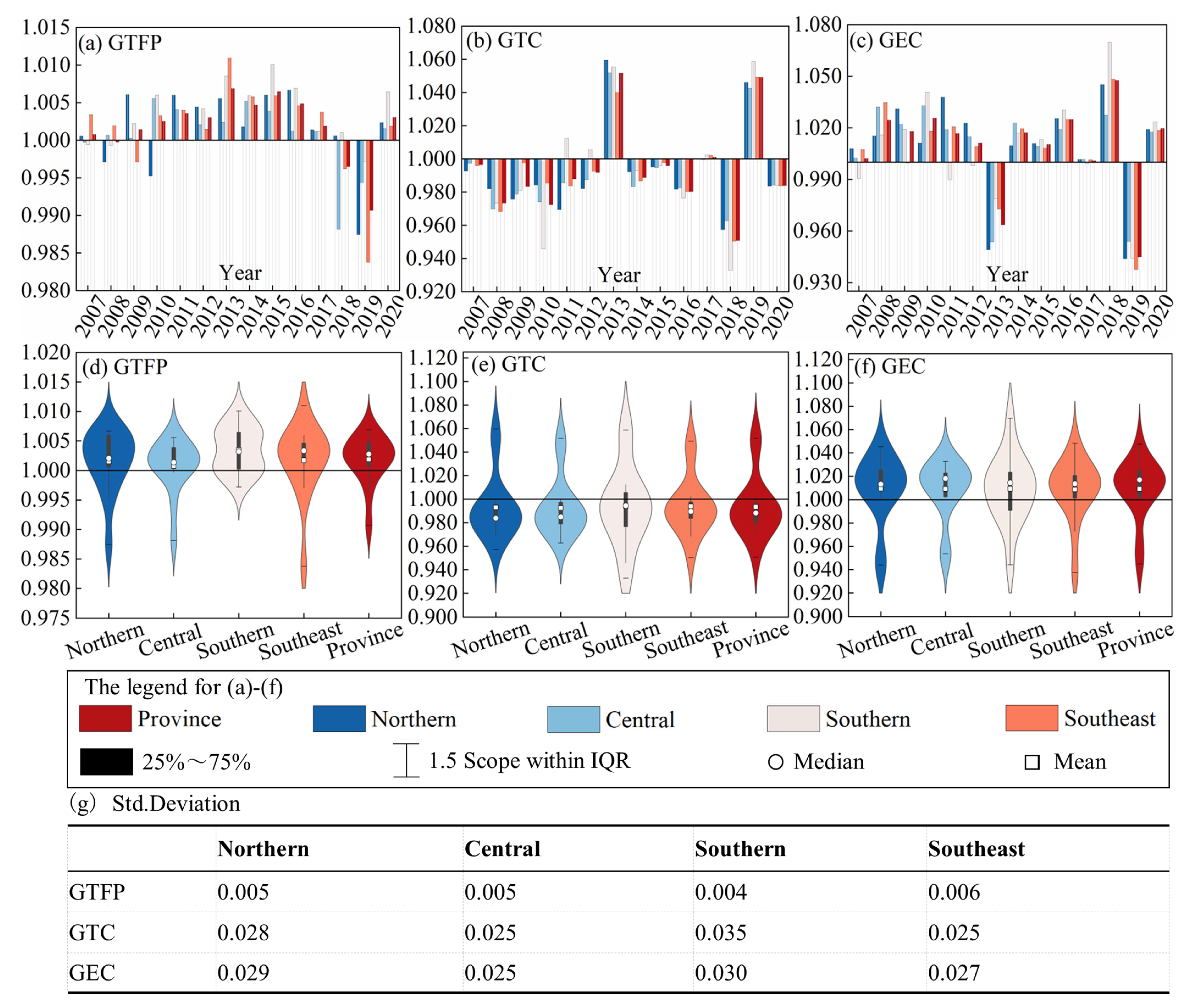
3.1. Analysis of the Evolution of HQED Efficiency and GSEB Growth Rate

3.1.1. HQED Efficiency

Provincial Level (Figure 3a–f): (1) The GTFP generally exceeded 1 at most time points, indicating an overall upward trend in the efficiency of HQED in Shanxi Province. Notably, GTFP values fluctuated around 1 during 2007–2010 and 2017–2020, with all values less than 1 in 2019. However, GTFP values were consistently greater than 1 during 2011–2016, suggesting a relatively stable upward trend during this period. (2) The GTC value exhibited a fluctuating upward trend from 2007 to 2013, followed by a fluctuating downward trend from 2013 to 2020. This trend is opposite to that of GEC values, suggesting a weakening of overall green technological progress in Shanxi Province after 2013 but an improvement in green efficiency progress.

Regional Level (Figure 3a–g): (1) The southern region ranks highest in terms of average and median GTFP and GTC values, indicating superior efficiency in HQED and green technological progress. Furthermore, the southern region has the smallest standard deviation of GTFP values and the largest standard deviation of GTC, suggesting the best stability in HQED efficiency but the worst in green technological progress. (2) The central region ranks lowest in average and median GTFP and GTC values, indicating relatively lower efficiency in HQED and green technological progress. However, it has the smallest standard deviation of GTC, suggesting minimal changes in green technological progress. Interestingly, while the average GEC values of all regions are equal, the central region has the largest median GEC and the smallest standard deviation, indicating more significant and stable progress in green efficiency. (3) The northern region has the smallest median GEC, indicating the least significant progress in green efficiency.

City Level: (1) In terms of GTFP (Figure 4), most cities have GTFP > 1 in 12 out of the 14 years studied, except for 2018 and 2019, where the majority of cities had GTFP < 1. This suggests that the efficiency of HQED in each city is generally improving. Cities with higher average and median GTFP values include Xinzhou, Lvliang, Yuncheng, and Jinzhong (Figure 5). (2) In terms of GTC (Figure 4), most cities have GTC < 1 in 12 out of the 14 years studied, except for 2013 and 2019, where all cities had GTC > 1. This indicates that the green technological progress of most cities is generally negative. Cities with relatively high average and median GTC values are Linfen and Yuncheng (Figure 5). (3) In terms of GEC (Figure 4), most cities have GEC > 1 in 12 out of the 14 years studied, except for 2013 and 2019, where all cities had GEC < 1. This suggests that the progress of green efficiency in each city is significant, underscoring the importance of improving green technological efficiency in promoting HQED. The city with the highest average and median GEC values is Jinzhong (Figure 5). (4) From the perspective of standard deviation (Figure 5), Yangquan has the most stable distribution of GTFP, GTC, and GEC data. Notably, the average and median GTC values of all cities are less than 1, while the GEC values are greater than 1, further indicating that regional green technological progress is insufficient, but green efficiency progress is significant.

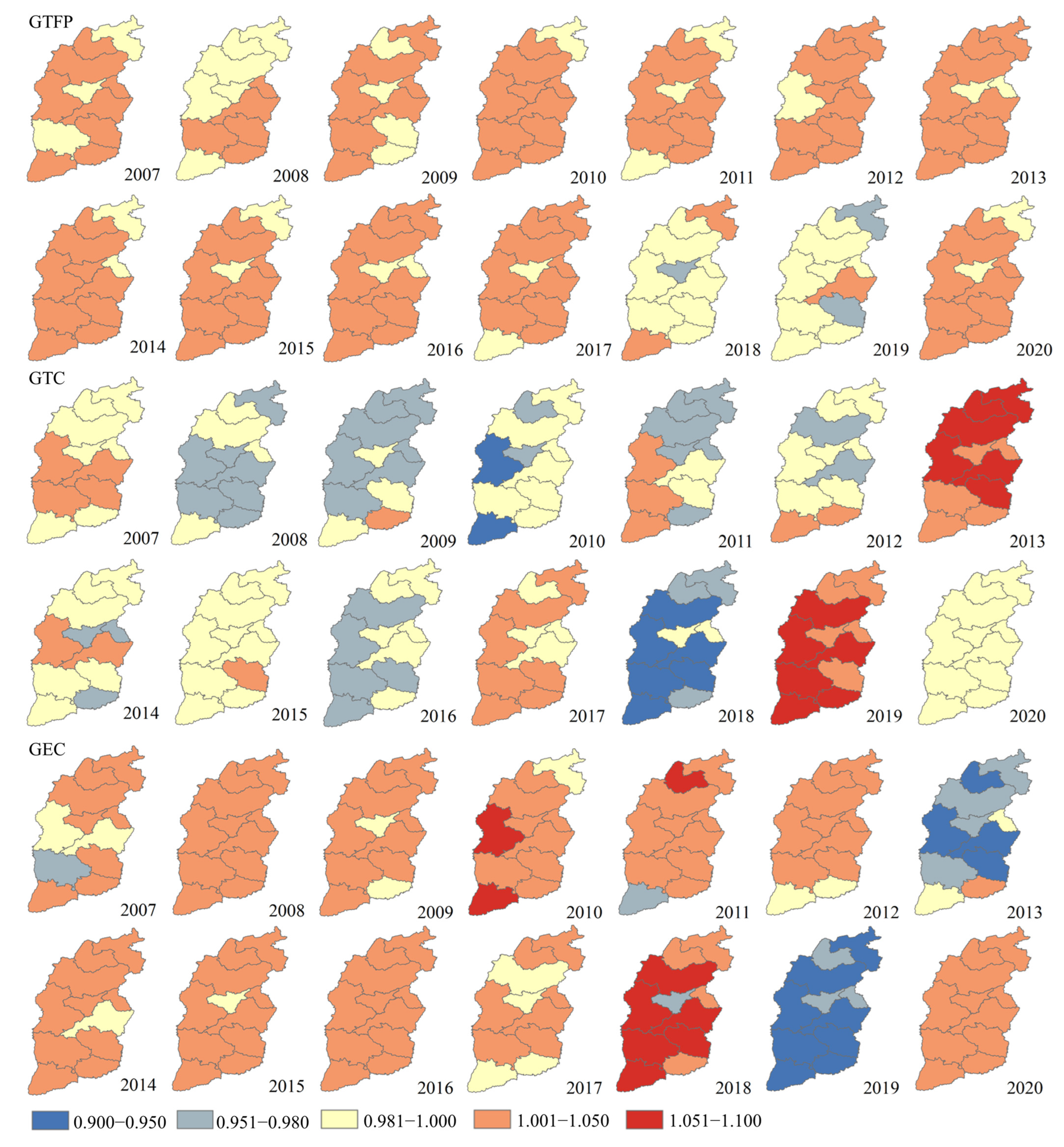
3.1.2. Evolution of Green Space Land Use and GSEB

Considering that the growth rate of GSEB (G_T) for the years 2007–2020 is derived from land-use changes and ecological benefits associated with green spaces during 2006–2020, the study conducts a systematic analysis of the evolution of land use (2006–2020), ecological benefits (2006–2020), and their respective growth rates for green spaces (2007–2020).

(1)

Land Use Evolution

Land Use Evolution in Shanxi Province (2006–2020) (Figure 6a,b): (1) Farmland exhibits a “decline → rise” trend during the study period, with an overall downward trend (growth rate of −0.06%). (2) Woodland shows a continuously increasing trend, with a growth rate of 11.96%. (3) Grassland displays a “growth → decline” trend, with a significant overall downward trend (growth rate of −12.08%). (4) Water Area demonstrates a continuous growth trend, with a growth rate of 15.46%.

As depicted in Figure 6c, the total area of land use transformation in Shanxi Province during the study period is 1.68 × 10⁴ km², with a net transfer from green space to non-green space of 2.16 × 10³ km². (1) Within Green Space: The most prominent land use type transfer is from grassland to woodland (4.41 × 10³ km²), indicating a transformation from an ecosystem with low service value to one with high service value. (2) From Green Space to Non-Green Space: The most significant transfers are from cultivated land to impervious surface (1.81 × 10³ km²) and from grassland to impervious surface (3.30 × 10² km²), suggesting that urban construction land primarily expands at the expense of farmland and grassland.

During the three periods (2006–2010, 2010–2015, and 2015–2020), the land use transformation was most significant in 2015–2020, with a transferred land area of 1.23 × 10⁴ km² (Figure 6b,c). This was mainly due to transfers from grassland to farmland (2.15 × 10³ km²), grassland to woodland (2.27 × 10³ km²), grassland to impervious surface (1.72 × 10² km²), and farmland to impervious surface (4.97 × 10² km²).

(2)

Evolution of GSEB and G_T

Provincial Level (Figure 7): (i) The GSESV per hectare in Shanxi Province exhibits a continuous growth trend. The total GSEB of the province increased by USD 0.95 billion (a total growth rate of 2.55%) during 2006–2020. (ii) The G_T of Shanxi Province fluctuated significantly from 2016 to 2020, reaching its highest in 2017 and lowest in 2019. (iii) According to the weights of various ecological functions (Table 3), the growth fluctuations of hydrological regulation and waste regulation values in the province’s green space from 2016 to 2020 are the most pronounced, while changes in cultural services (providing aesthetic landscapes) and maintaining nutrient cycling function values during the same period are relatively minor.

Regional Level (Figure 7): (i) The GSESV per hectare in southeast Shanxi is the highest and shows a continuous growth trend. The average value and standard deviation of G_T are the largest, indicating that the GSEB in the southeast are the most substantial and show a sustainable growth state. (ii) The GSESV per hectare in Central Shanxi ranks second, and the median of G_T is the largest. This suggests that the GSEB in the central part are second only to the southeast and, in most years, maintain a high ecological benefit growth trend. However, some years after 2012 have shown negative growth in GSESV, indicating a disruption in the stability of the ecological system function of the green space during this period. (iii) The GSESV per hectare in south Shanxi ranks second from the bottom, and the average of G_T are the smallest. This suggests that the GSEB in the south show a continuous loss trend. (iv) The GSESV per hectare in north Shanxi is the lowest, but it shows a continuous growth trend. This indicates that the total GSEB in the north are low, but the ecological system function shows a strengthening trend.

City Level (Figure 8a–c): (i) The GSESV per hectare in most cities changes slightly (the standard deviation is relatively small) and shows a growth trend in most years (G_T > 0), indicating that the GSEB of most cities are in a slow rising state. (ii) The GSESV per hectare in Jincheng always ranks first and shows a continuous growth trend (G_Tmin > 0), indicating that the GSEB in this city are the most prominent and show a sustainable development state. (iii) The GSESV per hectare in Yuncheng shows a downward trend in most periods (it has been continuously declining since 2012), and the average value and median of G_T are less than 0, indicating that the GSEB are declining most significantly. (iv) It is worth noting that the GSESV per hectare in Datong ranks second from the bottom, and the average value and median of G_T both rank second from the bottom, indicating that its GSEB status and development trend are unsustainable.

3.2. Analysis of the Coordinated Evolution of HQED and GSEB

3.2.1. Analysis of Coordination Degree Evolution

Provincial Level (Figure 9a–f): (1) Except for 2019, the GTFP-G_T coordination degree values of Shanxi Province in other years are consistently greater than 0.6, indicating that the overall coordination of HQED and GSEB in the province is above the primary level. (2) The GTC-G_T coordination degree values fluctuate around 0.6 (42.86% of the years are greater than 0.6), while the GEC-G_T coordination degree values are greater than 0.6 in most years (accounting for 85.71%). This suggests that the level of coordinated development of green technological progress and GSEB in the province is not stable (and overall below the primary coordination level), while the coordination level of green efficiency progress and GSEB is generally above the primary level.

Regional Level (Figure 9a–g): (1) The overall coordination levels of GTFP-G_T, GTC-G_T, and GEC-G_T in the southeast are all ahead of other regions (the number of years with coordination degree values less than 0.6 is the least). This indicates that the coordination level of HQED and GSEB in the southeast is the highest and relatively stable. (2) The overall coordination levels of GTFP-G_T, GTC-G_T, and GEC-G_T in the south are all behind other regions (the number of years with coordination degree values less than 0.6 is the most). This suggests that the coordination level of HQED and GSEB in the south is not only the lowest but also the most unstable.

City Level (Figure 10 and Figure 11): (1) The GTFP-G_T coordination degree values of each city are always greater than 0.6 throughout the year, indicating that the overall coordination of HQED and GSEB is above the primary level. However, there are also individual cities where the GTFP-G_T coordination degree values plummet in a few years (such as 2015, 2018, and 2019). (2) The average and median GTFP-G_T coordination degree values of all cities are at the primary coordination level and above. Among them, the average (0.760) and median (0.760) of Xinzhou are the largest, indicating that its coordination level of HQED and GSEB is the highest. (3) The size of the standard deviation indicates that the GTFP-G_T coordination level of Datong is the most unstable, the GTC-G_T coordination level of Yuncheng is the most unstable, and the GEC-G_T coordination level of Lvliang is the most unstable. It is worth noting that the average and median GTFP-G_T, GTC-G_T, and GEC-G_T coordination degree values of Yuncheng are all the smallest, and the standard deviation values of the three coordination degrees all rank in the top three, indicating that its coordination of HQED and GSEB is the lowest and shows an unstable evolution trend.

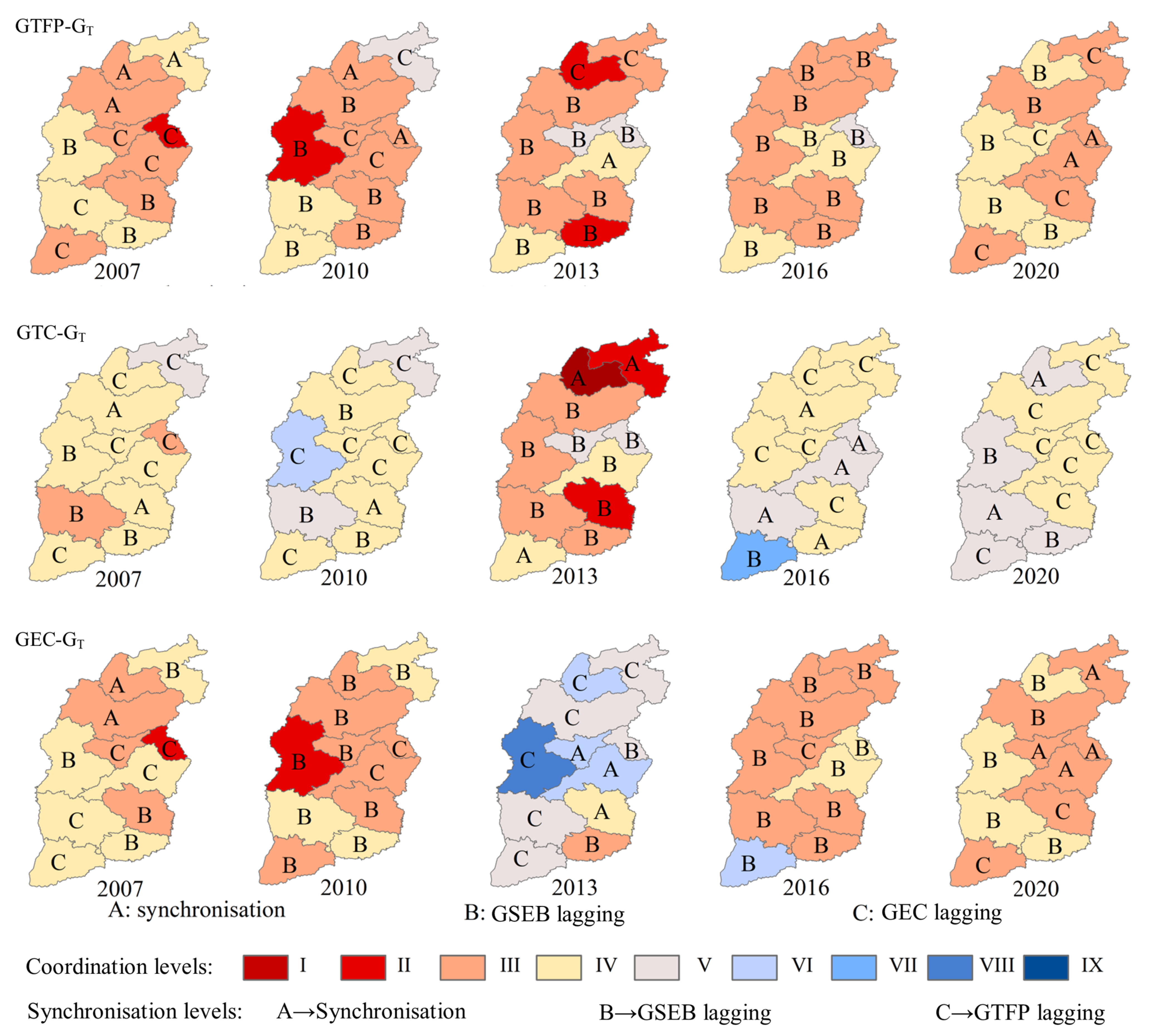
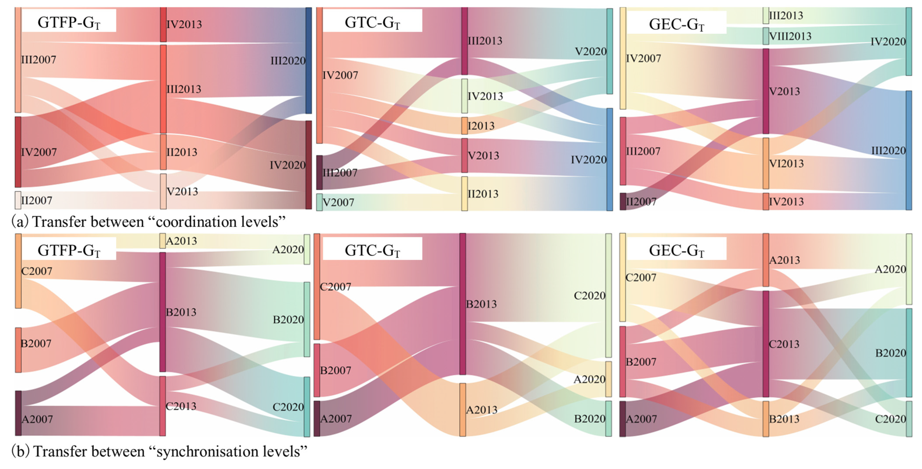
3.2.2. Evolution Analysis of Coordination Level and Synchronization Level

Selecting 2007, 2010, 2013, 2016, and 2020 as time nodes, an evolution analysis of the coordination level and synchronization level is conducted for cities. Selecting 2007, 2013, and 2020 as time nodes, a transfer flow analysis of the coordination level and synchronization level is conducted for cities.

(1)

GTFP-G_T

As shown in Figure 12, all cities are at “On the Verge of Discord V” and above from 2007 to 2020, and most are at “Intermediate Coordination III”, indicating that there is always a certain degree of coordination between HQED and GSEB in each city. As shown in Figure 13a, compared with 2007, the number of cities at level III remained unchanged in 2020, and one city was net transferred from level II to level IV. As shown in Figure 12 and Figure 13b, compared with 2007, the number of “Synchronous (A)” and “GTFP Lagging (C)” cities decreased by 1 in 2020, and the number of “GSEB Lagging (B)” cities increased by 2, indicating that the leading advantage of HQED in Shanxi Province over GSEB is still expanding.

(2)

GTC-G_T

As shown in Figure 12, compared with 2007, the coordination level of 6 cities declined in 2020, indicating that the coordination of green technological progress and GSEB in most cities in Shanxi Province has significantly declined. However, it is worth noting that in 2013, the proportion of cities at level III and above reached 63.64%, indicating that the coordination level of green technological progress and GSEB in most cities improved in the short term in 2013. As shown in Figure 13a, the number of cities from IV to III was the most (three) from 2007 to 2013, and the number of cities from III to V was the most (three) from 2013 to 2020. As can be seen from Figure 12 and Figure 13b, compared with 2007, the number of “Synchronous (A)” cities increased by 2 in 2020, the number of “GSEB Lagging (B)” cities increased by 1, and the number of “GEC Lagging (C)” cities all decreased by 3, indicating that the synchronization of green efficiency progress and GSEB in some cities in Shanxi Province is strengthening, but overall, the growth rate of GSEB is faster.

(3)

GEC-G_T

As can be seen from Figure 12, compared with 2007, the number of cities at level III and above increased by 3 in 2020, indicating that during the research period, the coordination of green efficiency progress and GSEB in some cities in Shanxi Province has been improved. However, it is worth noting that 91% of the cities experienced a downgrade in 2013, indicating that the GEC-G_T coordinated development level of most cities is not completely stable. As shown in Figure 13a, the number of cities from IV to V was the most from 2007 to 2013, and the number of cities from V to III was the most from 2013 to 2020. As can be seen from Figure 12 and Figure 13b, compared with 2007, the number of “Synchronous (A)” cities increased by 2 in 2020, the number of “GSEB Lagging (B)” cities increased by 1, and the number of “GEC Lagging (C)” cities all decreased by 3, indicating that the synchronization of green efficiency progress and GSEB in some cities in Shanxi Province is strengthening, but overall, the growth rate of GSEB is faster.

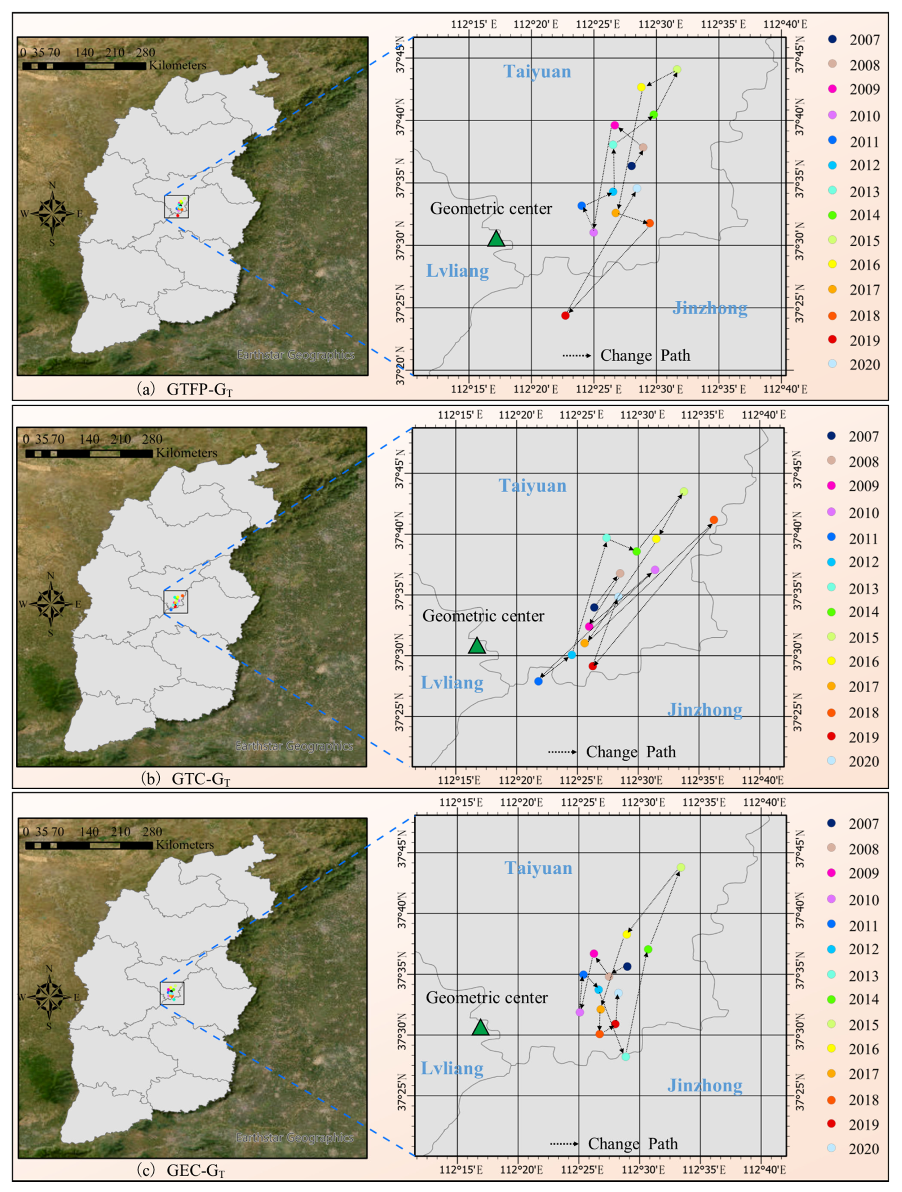
3.2.3. Spatial Balance Analysis of the Degree of Coordination

As can be seen from Figure 14a–c, from 2007 to 2020, the center of gravity of the coordinated evolution of HQED and GSEB in Shanxi Province was consistently located east of the geometric center of the administrative range (37°34′18″ N, 112°17′24″ E), with a relatively large distance from the geometric center. The center of gravity and the geometric center primarily experience a “close → far” trend.

(1)

The GTFP-G_T center of gravity is mainly distributed between 37°24′28″ N–37°43′37″ N, 112°22′54″ E–112°32′45″ E, and it shifts a short distance to the south as a whole. The annual average deviation of the GTFP-G_T center of gravity from the geometric center of Shanxi Province in each year is 20.71 km, with the maximum value in all years (35.78 km in 2015) being 2.64 times the minimum value (13.57 km in 2011). The direction of the center of gravity shift is generally north–south, but it is further away from the geometric center in 2020 than in 2007.

(2)

The GTC-G_T center of gravity is mainly distributed between 37°27′19″ N–37°43′54″ N, 112°22′13″ E–112°36′57″ E, and it shifts a short distance to the east as a whole. The annual average deviation of the GTC-G_T center of gravity from the geometric center of Shanxi Province in each year is 23.30 km, with the maximum value in all years (39.66 km in 2018) being 2.30 times the minimum value (17.27 km in 2012). The direction of the center of gravity shift is generally east–west, but it is further away from the geometric center in 2020 than in 2007.

(3)

The GEC-G_T center of gravity is mainly distributed between 37°28′15″ N–37°44′19″ N, 112°25′13″ E–112°33′10″ E, and it shifts a short distance to the south as a whole. The annual average deviation of the GEC-G_T center of gravity from the geometric center of Shanxi Province in each year is 21.37 km, with the maximum value (37.35 km in 2015) being 2.48 times the minimum value (15.06 km in 2010). The direction of the center of gravity shift is generally north–south, but it is closer to the geometric center in 2020 than in 2007.

3.2.4. Heterogeneity and Homogeneity in the Levels of Coordinated Development

(1)

Inter-Regional Heterogeneity

Based on the calculation results of the Theil index (Figure 15), the coordination degree between HQED and GSEB in Shanxi Province from 2007 to 2020 shows a fluctuating trend. Among these, the fluctuation trend of the three types of coordination degrees is most evident from 2013 to 2020. Additionally, there are significant differences between intra-regional and inter-regional coordination degrees, with inter-regional differences being the main source of overall differences from 2007 to 2020. It is noteworthy that the differences in the three types of coordination degrees within each region are not significant at most time points, but the differences in the three types of coordination degrees among cities in southern Shanxi Province were significantly higher than those in other regions from 2015 to 2016.

(2)

Inter-Regional Homogeneity

Figure 16a–c illustrates the evolution of coordination degrees from 2007 to 2020. The number of cities with significant correlations in the three coordination degrees is ranked as follows: GEC-E_T > GTC-E_T > GTFP-E_T. This suggests that while there are fewer cities with similar trends in the coordinated evolution of HQED and GSEB, more cities exhibit similar trends in the coordinated evolution of green technological efficiency progress and GSEB. In the GTFP-G_T coordinated evolution, Yangquan–Jinzhong, Linfen–Lvliang, Jincheng–Xinzhou, and Shuozhou–Changzhi show the most similar trends, while Yangquan and Jincheng display opposite trends. In the GTC-G_T coordinated development, Yangquan–Taiyuan, Lvliang–Linfen, Shuozhou–Datong, Xinzhou–Changzhi, and Shuozhou–Xinzhou exhibit the most similar trends, whereas Datong and Yangquan show opposite trends. In the GEC-G_T coordinated development, Shuozhou–Datong, Linfen–Xinzhou, Changzhi–Jinzhong, Changzhi–Taiyuan, and Linfen–Taiyuan have the most similar trends, with no city showing an opposite trend to others.

Further cluster analysis, integrating the correlation results and the evolution trend of coordination degree, suggests a reasonable division of the cities into five categories, represented as Cluster1–5. These clusters are assigned meanings corresponding to declining overall coordination levels (Figure 16a–c). Overall, the classification results of the three coordination degrees vary, with Cluster1 of the GEC-G_T coordination degree containing the most cities (six). This indicates that most cities in Shanxi Province have better coordination between green technological efficiency and GSEB. Notably, both Xinzhou and Changzhi belong to Cluster1 in all three coordination degrees, suggesting that these two cities have a higher overall coordination level of HQED and GSEB than other cities, with the coordinated evolution trend showing clear fluctuations.

3.3. Driving Mechanism of Coordinated Evolution at Multiple Scales

3.3.1. Driving Influence of Provincial and Regional Levels

Provincial Level: Figure 17a reveals that 73.33% of the key driving indicators have a correlation value greater than 0.8 with the three coordination degrees, suggesting that most driving indicators strongly influence the province’s three coordination degrees. Figure 17b shows that all driving factors have a weight greater than 0.1, indicating their significance in driving the coordinated evolution of HQED and GSEB in Shanxi Province.

Regional Level: (1) Northern Shanxi Province: Figure 17a,b shows that the park green space area (B₁₄) has the most significant role in promoting the coordinated evolution of HQED and GSEB in the northern region. The annual GDP growth rate (B₂) has the weakest driving influence. (2) Central Shanxi Province: As shown in Figure 17a,b, the important driving indicators with a correlation degree greater than 0.8 with the three coordination degrees are per capita science and technology expenditure (B₅) and the number of patent authorizations (B6), highlighting the important impact of scientific and technological innovation on promoting the coordinated evolution of HQED and GSEB in central Shanxi. (3) Southern Shanxi Province: As shown in Figure 17a,b, the important driving indicator with a correlation degree greater than 0.8 with the three coordination degrees is only the average number of college students per 10,000 people (B₁₀), indicating that highly educated human resources have the greatest driving force for the coordinated evolution of HQED and GSEB in the south. (4) Southeastern Shanxi Province: As can be seen in Figure 17a,b, the proportion of important driving indicators with a correlation of more than 0.8 to the three degrees of coordination is 53.33 percent, and the correlation values of these indicators are all greater than 0.9, which highlights the fact that the driving indicators for the coordinated evolution of HQED of the south-east and the GSEB are not only the most numerous, but also have a strong influence.

3.3.2. Driving Influence of Cities

As depicted in Figure 18a, the same driving indicator exhibits significant differences in correlation values at the regional and city scales. However, they all share a common characteristic: the correlation values of the three coordination degrees with the same driving indicator are closely aligned. This could be due to the fact that both GTC and GEC are decomposed from GTFP. Notably, B₃ (the proportion of the output value of the tertiary industry) and B₄ (the advanced level of industrial structure) are key driving indicators for promoting the coordinated development of GTFP-G_T, GTC-G_T, and GEC-G_T across all cities, with correlation values greater than 0.8 and less than or equal to 1.

Further calculations of the weight values of seven driving factors across 11 cities (detailed in Figure 18b) reveal that the weight of the seven driving factors in each city is greater than 0.11. This indicates that each driving factor significantly impacts the three coordination degrees of the city. The polarization of the weight values is not pronounced, suggesting a balanced influence of all driving factors. For all cities, A₆ (industrial “three wastes” governance) and A₂ (industrial transformation) consistently rank in the top three driving factors. The importance ranking of other driving factors varies from city to city, indicating that comprehensive industrial pollution control and industrial transformation optimization are essential measures to promote the coordinated evolution of HQED and GSEB in Shanxi Province and its cities. Additionally, we found that the proportion of important indicators in the driving indicators of GTFP-G_T, GTC-G_T, and GEC-G_T coordinated evolution in Jincheng reached 100%. The range of the weight of each driving factor was the smallest, indicating that all driving factors have a significant impact on Jincheng. This suggests that Jincheng’s coordinated evolution is strongly influenced by all driving factors.

4. Discussion

4.1. Efficiency of HQED

(1)

The overall efficiency of HQED in various regions of Shanxi Province is on the rise, which reflects the policy effectiveness of China’s implementation of the “14th Five-Year Plan” for promoting high-quality development in resource-based areas (https://www.fj.gov.cn/english/news/202108/t20210809_5665713.htm (accessed on 6 October 2024)). The level of green technology progress in most regions of the province has declined during most time points, but the efficiency of green technology has improved. This indicates that during this period, the efficiency of green technology has compensated for the shortcomings of green technology progress, which is an important driving force for promoting HQED in the region. Therefore, to achieve the sustainability of HQED in the region, the key is to promote its green technology progress.

(2)

The years 2013 and 2019 are two time points worth noting. The GTC of most cities has significantly increased and is greater than 1, and the GEC has significantly decreased and is less than 1. This is contrary to the development trend in other years. The important driving force for promoting HQED in the region has shifted from green technology efficiency to green technology progress. The possible reason for this phenomenon is the short-term effect of policy guidance. (i) In November 2012, the Chinese government determined the policy of regional ecological civilization construction. Subsequently, at the 27th Council of the United Nations Environment Programme (UNEP) held in February 2013, China’s ecological civilization concept was officially written into the decision document. Against this background, Shanxi Province proposed the Chinese coal industry development standard system for the first time in 2013, laying a theoretical foundation for green coal mining. At the same time, the government vigorously implemented the innovation-driven development strategy, strengthened the construction of scientific and technological innovation platforms, and vigorously promoted comprehensive ecological governance projects such as ecological environment, which led to the most significant progress in green technology development in 2013. (ii) In 2018, the Shanxi provincial government reduced corporate taxes and administrative fees by 57.3 billion CNY, leaving more funds for green technology reform for various enterprises (http://english.scio.gov.cn/pressroom/2019-09/06/content_75190976.htm (accessed on 2 October 2024)). According to statistics, the annual growth rate of R&D investment in large state-owned enterprises in Shanxi Province reached 18.5% from 2018 to 2019 (https://english.www.gov.cn/). In 2019, the policy of “accelerating the development of advanced manufacturing and other emerging industries and establishing a modern industrial system in Shanxi Province” was proposed at the press conference of the State Council Information Office of China, which once again led to further improvement in regional green technology. (iii) Considering the existing scientific research potential, energy and industrial structure, financial development and foreign trade, etc., in Shanxi Province [76], the development and use of new technologies still face problems such as funds and scientific research level, and the sustainability of green technology progress is not stable. At the same time, the promotion of green technology may bring some distribution problems, such as it may affect the interests of certain industries or groups, which will lead to a slowdown in R&D progress and an increase in costs, resulting in a temporary decrease in green technology efficiency.

4.2. GSEB Evolution

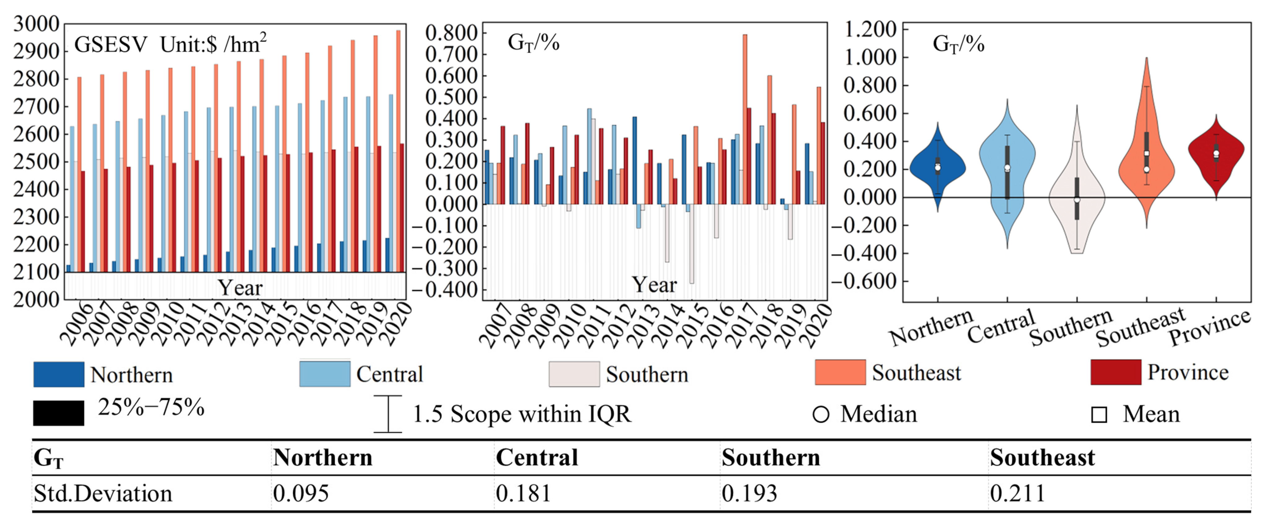
(1)

Although the total area of green space in Shanxi Province decreased from 2006 to 2020, the GSEB showed a continuous upward trend. The main reason may be that the area decline in the green space only includes cultivated land and grassland, which are two ecosystems with lower service value equivalents, while the area of forest land and water bodies, which have higher service value, shows a fluctuating increase trend.

(2)

The GSESV and G_T per hectare in the southeast are the highest. The main reason is that the area of forest land and water bodies in the southeast is growing continuously. Compared with 2006, the area of forest land and water bodies increased by 1.13 × 10⁵ hm² and 870.3 hm^2, respectively, in 2020. The GSESV per hectare in the central part showed a fluctuating trend after 2012, which was mainly caused by the decline in the area of grassland in this region in 2013, 2014, 2015, and 2019 (decreasing by 2.87 × 10⁴ hm², 4.40 × 10³ hm², 8.93 × 10³ hm², 5.03 × 10⁴ hm², respectively). Similarly, the main reason for the perennial negative growth of the GSESV in the south is also the large decline in the area of grassland. The possible reason for the decline in the area of grassland is the decrease in precipitation in the region. A decrease in precipitation is one of the important factors leading to grassland degradation [77], and the precipitation in the south and central parts of Shanxi Province decreased significantly during this period [78]. In addition, it was found that the GSESV per unit area in the north is the lowest, but it shows a weak strengthening trend. The main reason is that the green space in the north is mainly composed of cultivated land and grassland, which are two ecosystems with lower GSESV equivalents, while the area proportion of water bodies and forest land, which have higher GSESV equivalents, is smaller.

(3)

From 2006 to 2020, the overall decline in the GSESV value in Yuncheng was the most obvious. The direct reason is the significant decline in the area of forest land and grassland (decreasing by 8.16 × 10³ hm² and 2.75 × 10⁴ hm², respectively), and the increase in the area of water bodies and cultivated land is less (increasing by 1.93 × 10³ hm² and 2.97 × 10³ hm², respectively). In addition, the GSESV of Xinzhou, Jincheng, and Changzhi showed a continuous growth trend, which mainly benefited from the large increase in the area of forest land ecosystem. During the research period, the increase in forest land area in Xinzhou, Jincheng, and Changzhi was 7.69 × 10⁴ hm², 5.35 × 10⁴ hm², and 5.93 × 10⁴ hm², respectively.

4.3. Coordinated Evolution of HQED and GSEB

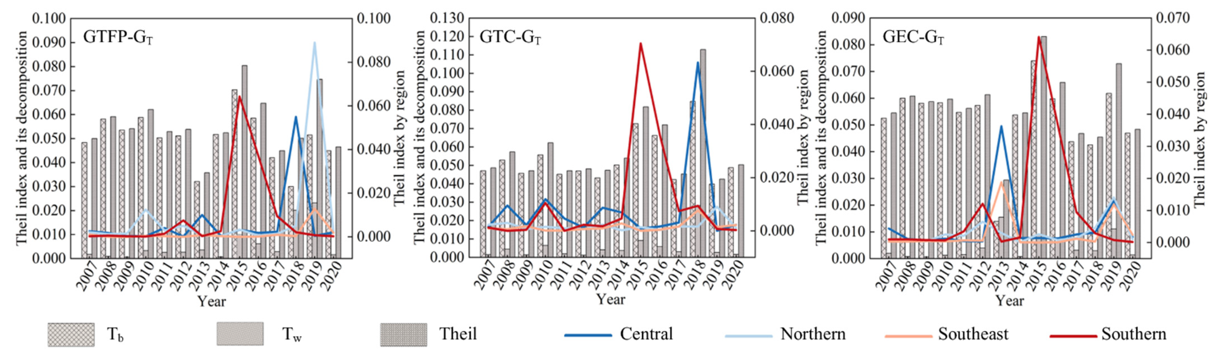
(1)

Provincial Level: The overall coordination of HQED and GSEB in Shanxi Province is above the primary level. However, in 2019, the coordination degree of the two was slightly lower than the primary coordination level, likely due to the significant decline in GTFP in that year. Additionally, the green technology progress and green space ecological benefits are below the primary coordination level at most times, exhibiting obvious volatility, which may be attributed to the volatility and lag of GTC. The overall coordination level of green technology efficiency and GSEB in the province is above the primary coordination level, but the coordination of the two is below the primary coordination level in 2013 and 2019, which may be caused by the significant decline in GEC in 2013 and 2019.

(2)

Regional Level: The synergy level of HQED and GSEB presents a spatial pattern of “highest in the southeast, followed by the central and northern parts, and lowest in the south”. During the research period, except for the GTC-G_T in the south, which is generally below the primary coordination level, the overall level of the three coordination degrees in other regions reached or exceeded the primary coordination. The three coordination development levels in the southeast are the highest, primarily because the average and median values of GTFP, GTC, and GEC in this region are all ranked in the top two, and the average value of G_T ranks first. The overall coordination development level in the south is the lowest, likely because the average values of GTFP, GTC, and GEC in this region from 2007 to 2020 are all the highest, while the average value of G_T is the lowest, indicating a large gap between the HQED and GSEB.

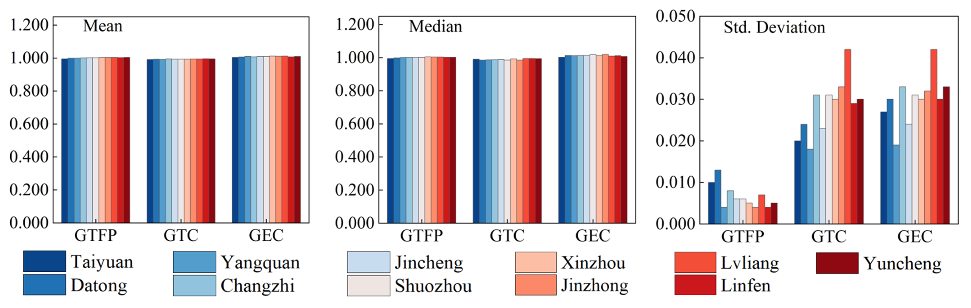
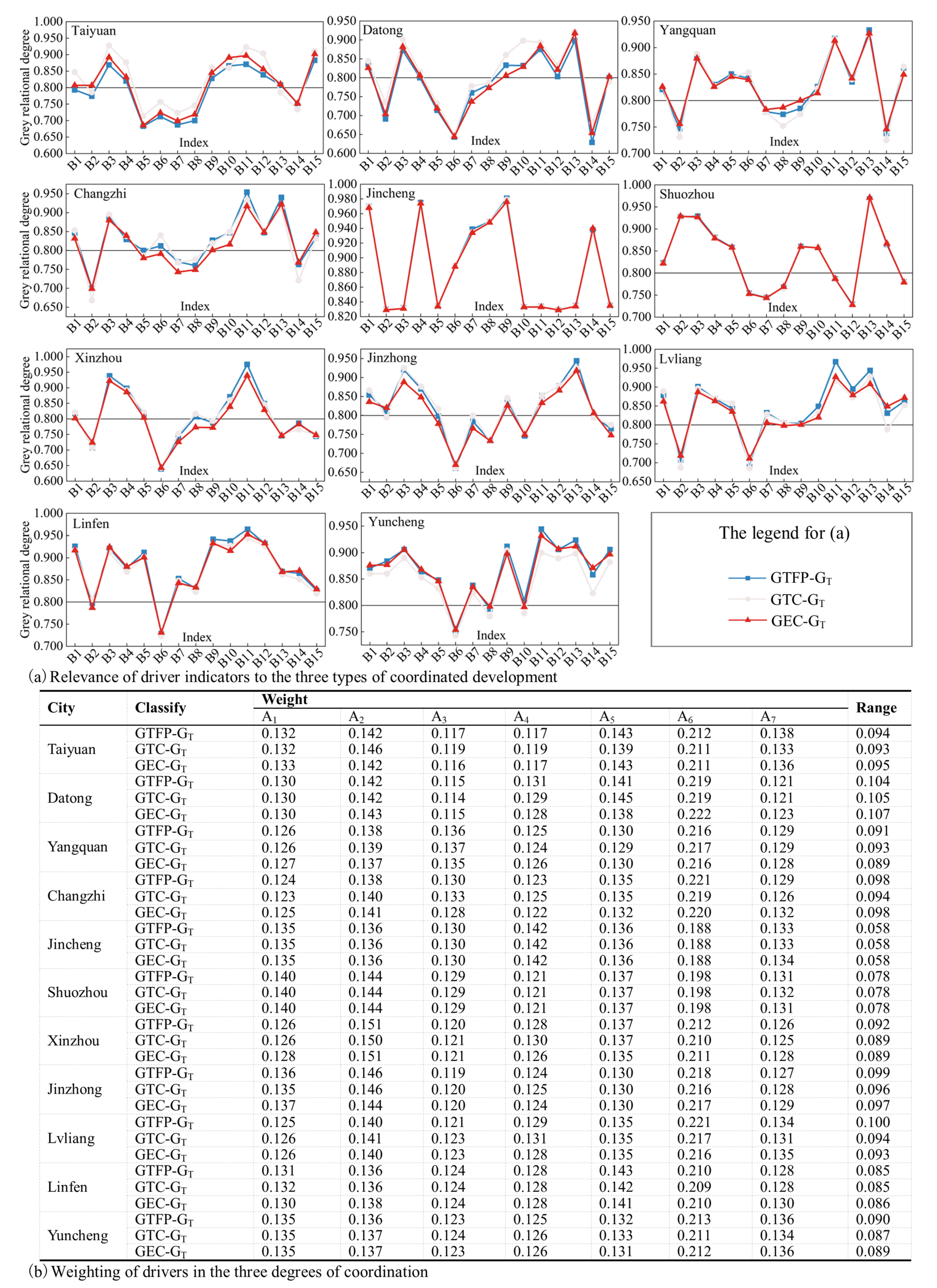
(3)

City Level: During the research period, Xinzhou’s efficiency of HQED and green technology efficiency both have higher coordination with GSEB. The main reason may be that the overall level of GTFP, GEC, and G_T in Xinzhou from 2007 to 2020 is the highest, and the trend of change is stable. Jincheng and Changzhi have higher coordination between green technology progress and GSEB, mainly because the numerical changes of GTC and G_T in Jincheng show larger volatility, while the numerical change trends of GTC and G_T in Changzhi are more stable. We also found that the three coordination development levels of Yuncheng are all the lowest and all show unstable evolution trends. Among them, the low coordination of GTFP-G_T and GTC-G_T is due to the high overall level of HQED and green technology progress in this city, while the overall G_T is the lowest. In addition, the reason for the low coordination of GEC-G_T is that the development trend of green technology efficiency in this city is stable, while the development trend of GSEB is more volatile. It is worth noting that Datong and Yangquan have a negative correlation; the main reason is that the development trends of these two cities are completely opposite. Among them, the overall change trend of GTC-G_T in Datong is “first rise → then fall”, while the overall change trend in Yangquan is “first fall → then rise”.

4.4. Driving Mechanism of Coordinated Evolution

The correlation degree of all indicators with the three coordination degrees at all scales exceeds 0.6. This suggests that the selected driving indicators are representative at all scales, and the constructed driving factor indicator system is reasonable. Interestingly, for the same city, region, and province, the important driving indicators and the top three driving factors of GTFP-G_T, GTC-G_T, and GEC-G_T are consistent. This consistency may be attributed to the fact that GTC and GEC are decomposed from GTFP, and the three are interrelated. Based on this result, we collectively refer to the three coordination evolutions as the “coordinated evolution of high-quality economic development and green space ecological benefits (C-HQED-GSEB)” and discuss its main driving factors.

(1)

Industrial “Three Wastes” Governance: This is the most significant driving force for the C-HQED-GSEB across all cities in Shanxi Province. The industrial structure of all cities in Shanxi Province is dominated by heavy industry, primarily concentrated in coal, alumina, coke, steel, power, and other energy industries, as well as high-energy-consuming industries (http://www.leadingir.com/hotspot/view/3468.html (accessed on 6 October 2024)). These industries produce a large amount of industrial “three wastes”, which have a substantial negative impact on green development and ecosystem services. Therefore, the governance of industrial “three wastes” has a significant driving effect on the coordinated evolution of C-HQED-GSEB. On the one hand, some waste in industrial “three wastes” can be recycled and reused through technological means, transforming it into valuable resources, which is an important method of achieving green development [79]. In addition, the governance of industrial “three wastes” can promote the green transformation of industrial production methods, improve the level of green technology, and be conducive to promoting high-quality economic development [80]. On the other hand, effective industrial “three wastes” governance can reduce the emission of waste gas, wastewater, and waste residue, reduce environmental pollution, and improve the quality of the ecological environment, which is conducive to maintaining the stability of the ecosystem and providing better ecosystem services and more ecological benefits [81].

(2)

Industrial Transformation: This factor has a significant driving effect on the C-HQED-GSEB across all cities in Shanxi Province. The proportion of heavy industry in all cities in Shanxi Province is substantial, and the industrial structure is unbalanced, which is not conducive to the region’s sustainable development. On the one hand, industrial transformation can promote the development of green industries, such as the development of energy-saving and environmental protection industries and clean energy industries [82]. It can also promote the optimization of the energy structure, such as vigorously developing clean energy and reducing dependence on fossil energy [83]. Furthermore, it can guide green consumption, such as encouraging the use of new energy vehicles and the adoption of new materials that are less harmful to the human body [84]. It can also promote the innovation of green technology, such as realizing the intelligence of traditional industries and building a low-consumption and high-yield green manufacturing system [85]. All these factors greatly promote the HQED of cities. On the other hand, industrial transformation also includes optimizing the layout of national spatial development and adjusting the industrial layout of regional basins. This optimization can produce more GSEB by protecting and restoring ecosystems [86].

(3)

Innovation Input–Output: This factor has a larger driving effect on the C-HQED-GSEB in the central, southern, and southeast cities of Shanxi Province but has a relatively weak impact on southeast cities. The positive driving effect of innovation input–output on HQED and GSEB has been confirmed by many studies. On the one hand, innovation input–output has a significant role in promoting green technology innovation [87], optimizing production processes [88], promoting the development of green products and services [89], and promoting the development of green finance [87], etc.; all of these are conducive to achieving regional HQED. On the other hand, innovation input can enhance the ecosystem service value of green space [90] and improve the efficiency and effect of ecosystem services of green space [91]. This study shows that innovation input–output has a significant difference in driving C-HQED-GSEB in various regions of Shanxi Province. We found that this trend is strongly correlated with the number of undergraduate colleges (with the right to grant bachelor’s degrees) in each region. According to official statistics from the Ministry of Education of China (http://en.moe.gov.cn/), the average number of undergraduate colleges in each city in central Shanxi ranks first (6), followed by the south (2) and the southeast (1.5), and the north ranks last (1). Therefore, the main reason for the regional difference in the driving impact of innovation input–output may be the spatial distribution difference of higher education level because areas with a high level of education have more highly skilled talents and R&D personnel, which is more conducive to improving the effect of innovation input–output [92].

(4)

All Driving Factors: The research results reveal that, in addition to the aforementioned three driving factors, the C-HQED-GSEB in Jincheng, located in the southeast of Shanxi Province, are significantly influenced by economic level, human resources, construction investment, and improvement of living environment.

(i) The improvement of economic level has a positive impact on regional green development [93] and can indirectly enhance the service value of the green space ecosystem [94]. According to the data from the China City Statistical Yearbook, Jincheng’s per capita GDP has long been leading among all cities in Shanxi Province. (ii) Human resources also drive regional green development and the service of green space ecosystems [95,96]. In recent years, Jincheng has vigorously introduced talents related to environmental protection, providing human resource guarantees for regionally coordinated development. (iii) Construction investment can also promote regional green development and the perfection of ecosystem service function [97,98]. According to data from the China City Statistical Yearbook, we found that fixed asset investment in Jincheng in 2020 increased by 1123.78% compared with 2007, of which environmental protection investment exceeded 50%, injecting strong momentum into the driving of coordinated development by construction investment. (iv) The process of improving the living environment also promotes the HQED and the enhancement of ecosystem services in the region [99,100]. According to data from the China City Statistical Yearbook, the area of urban park green space in Jincheng in 2020 increased by 112.46% compared with 2007, and the harmless treatment rate of domestic garbage increased from 90% in 2007 to 100% in 2020, which greatly promoted the sustainable development of the region.

Based on the important driving indicators and main driving factors at all scales, a driving mechanism diagram of C-HQED-GSEB in Shanxi Province is further formed (as shown in Figure 19).

4.5. Policy Suggestions

In 2021, the Shanxi Provincial Government released the “14th Five-Year Plan for National Economic and Social Development and the Long-Range Objectives Through the Year 2035”. Although this document highlights key goals such as promoting high-quality economic development and enhancing ecosystem quality, there is still a lack of dedicated spatial planning or policies for sustainable development. This study thoroughly analyzes the coordinated evolution patterns of HQED and GSEB at different spatial scales in Shanxi Province from 2007 to 2020. This analysis helps policymakers identify the balance between economic development and environmental protection. To address the gap in sustainable development spatial planning in Shanxi Province, we have preliminarily proposed the “Shanxi Province 2035 Sustainable Development Vision Plan” based on the coordinated evolution of HQED and GSEB.

The main content includes, firstly, that Shanxi Province should restrict urban expansion to prevent cultivated land and grassland from being replaced by urban construction land. Secondly, considering that the spatial differences in the coordination between HQED and GSEB in Shanxi Province primarily stem from inter-regional disparities, we have categorized the regions into three groups based on the C-HQED-GSEB sequence from low to high: priority development, sub-priority development, and steady development. Furthermore, we have identified the regions that should be prioritized for improvement based on their synchronization levels. (1) The southern part is a priority development area, and the future policy inclination of the Shanxi government for its coordinated development is the largest. The city with the lowest level of coordinated development is Yuncheng, which should prioritize the improvement of green space ecological benefits. (2) The central and northern parts belong to the secondary priority development area. The future policy inclination of the Shanxi provincial government for its coordinated development is only second to the south. The cities with the lowest level of coordinated development in the central and northern parts are Taiyuan and Datong, respectively, both of which should prioritize the improvement of high-quality economic development efficiency, especially the rapid progress of green technology. (3) The southeast belongs to steady development. The future policy inclination of the Shanxi provincial government for its coordinated development is lower than the other three regions. The city with the lowest level of coordinated development is Changzhi, which should prioritize the improvement of green space ecological benefits. The detailed policy is shown in Figure 20.

4.6. Limitations and Uncertainties

The original data collected for this study primarily span the period from 2006 to 2020 (used for calculating HQED and GSEB from 2007 to 2020) or from 2007 to 2020 (used for analyzing driving factors). It is acknowledged that the selection of data inevitably involves a certain degree of lag. Although these data are sufficient to reveal the synergistic evolution characteristics and driving factors of high-quality economic development and the ecological benefits of green spaces, they are insufficient to explain the current or future development trends of the study area. In the future, we anticipate further exploring the coordinated development patterns between the two under updated and longer time series of original data.

Moreover, although we have achieved relatively ideal research results, the limited length of the paper has resulted in a lack of predictive analysis of future development trends. Therefore, in subsequent research, we will simulate and predict the synergistic evolution characteristics of high-quality economic development and the ecological benefits of green spaces over the next decade and formulate sustainable development policies based on future trends. Finally, although this paper has provided a new perspective for global sustainable development research, it is still necessary to expand the research scope (e.g., to the entire region of China or globally) in the future to further enhance the impact of the research findings.

5. Conclusions

The coordinated evolution of high-quality economic development (HQED) and green space ecological benefits (GSEB) aids in the harmonious coexistence of humans and nature, promoting a shift in the global economic development mode and enhancing the level of ecological civilization. This study systematically investigates the spatiotemporal evolution characteristics and driving mechanisms of the coordinated evolution of HQED and GSEB in typical resource-based regions of China from 2007 to 2020 from different spatial scale perspectives. This comprehensive research approach is conducive to the formulation of sustainable development policies by governments at various administrative levels. The primary conclusions are as follows:

(1)

The efficiency of HQED in Shanxi Province has generally improved. Post-2013, GEC emerged as a significant driver for HQED. The southern region exhibited exceptional performance in GTFP and GTC.

(2)

The green space in Shanxi Province primarily transitioned from ecosystems with low service value to those with high service value. The GSESV per hectare consistently increased, with significant fluctuations in the growth rate of GSEB from 2016 to 2020. The southeast region recorded the highest GSESV per hectare, demonstrating an overall upward trend.

(3)

The spatial differences in the coordination between HQED and GSEB are most pronounced among regions. The southeastern region exhibits the highest overall coordination level, significantly surpassing other areas, while the southern region demonstrates the lowest and most unstable coordination level. The center of gravity of coordination has experienced a “proximity to distance” trend relative to the geometric center of Shanxi Province. Overall, the province’s HQED and GSEB are at a primary coordination level or above, with HQED leading GSEB. Notably, the co-evolution trend between green technological progress and GSEB is highly volatile, with the latter generally outpacing the former. In contrast, the synchronization between green technological efficiency and GSEB is more evident.

(4)

The governance of industrial “three wastes” and industrial transformation have consistently been crucial drivers for the coordinated evolution of HQED and GSEB across Shanxi Province’s spatial scale regions. The effect of innovation input–output was particularly pronounced in the central, southern, and southeastern parts of Shanxi Province.

References

- Giovannucci, D.; Scherr, S.; Nierenberg, N.; Hebebrand, C.; Shapiro, J.; Milder, J.; Wheleer, K. Sustainable Development in the 21st Century (SD21). In Food and Agriculture: The Future of Sustainability; UN: New York, NY, USA, 2012. [Google Scholar]
- Zhu, J.; Sun, X.; He, Z. Research on China’s sustainable development evaluation indicators in the framework of SDGs. China Popul. Resour. Environ. 2018, 28, 9–18. [Google Scholar]
- Wang, Y.; Guo, C.H.; Chen, X.J.; Jia, L.Q.; Guo, X.N.; Chen, R.S.; Zhang, M.S.; Chen, Z.Y.; Wang, H.D. Carbon peak and carbon neutrality in China: Goals, implementation path and prospects. China Geol. 2021, 4, 720–746. [Google Scholar] [CrossRef]
- Yin, K.; Han, R.; Huang, C. Effect on high-quality economic development of foreign direct investment in China from the triple perspectives of financial development. J. Clean. Prod. 2023, 427, 139251. [Google Scholar] [CrossRef]
- Van Beveren, I. Total factor productivity estimation: A practical review. J. Econ. Surv. 2012, 26, 98–128. [Google Scholar] [CrossRef]
- Chao, F.; Huang, J.; Wang, M. Analysis of green total-factor productivity in China’s regional metal industry: A meta-frontier approach. Resour. Policy 2018, 58, 219–229. [Google Scholar]
- Chen, S.; Yang, Y.; Wu, T. Digital economy and green total factor productivity—Based on the empirical research on the resource-based cities. Environ. Sci. Pollut. Res. 2023, 30, 47394–47407. [Google Scholar] [CrossRef] [PubMed]
- Jiang, R.; Yang, S.; Lian, S.; Jefferson, G.H. The impact of internet development on green total factor productivity in China’s prefectural cities. Inf. Technol. Dev. 2023, 29, 462–487. [Google Scholar] [CrossRef]
- Peng, Y.; Lin, H.; Lee, J. Analyzing the mechanism of spatial–temporal change of green total factor productivity in Yangtze Delta Region of China. Environ. Dev. Sustain. 2023, 25, 14261–14282. [Google Scholar] [CrossRef]
- Qian, Y.; Liu, J.; Forrest JY, L. Impact of financial agglomeration on regional green economic growth: Evidence from China. J. Environ. Plan. Manag. 2022, 65, 1611–1636. [Google Scholar] [CrossRef]
- Xu, X.; Yue, A.; Meng, X. Increase in Industrial Sulfur Dioxide Pollution Fee and Polluting Firms’ Green Total Factor Productivity: Evidence from China. Sustainability 2023, 15, 10761. [Google Scholar] [CrossRef]
- Chung, Y.H.; Färe, R.; Grosskopf, S. Productivity and undesirable outputs: A directional distance function approach. J. Environ. Manag. 1997, 51, 229–240. [Google Scholar] [CrossRef]
- Tone, K.; Tsutsui, M. An epsilon-based measure of efficiency in DEA–A third pole of technical efficiency. Eur. J. Oper. Res. 2010, 207, 1554–1563. [Google Scholar] [CrossRef]
- Luo, Y.; Mensah, C.N.; Lu, Z.; Wu, C. Environmental regulation and green total factor productivity in China: A perspective of Porter’s and Compliance Hypothesis. Ecol. Indic. 2022, 145, 109744. [Google Scholar] [CrossRef]
- Yu, B.; Fang, D.; Pan, Y.; Jia, Y. Countries’ green total-factor productivity towards a low-carbon world: The role of energy trilemma. Energy 2023, 278, 127894. [Google Scholar] [CrossRef]
- Oh, D.H. A global Malmquist-Luenberger productivity index. J. Prod. Anal. 2010, 34, 183–197. [Google Scholar] [CrossRef]
- Wang, X.; Zhu, Y.; Ren, X.; Gozgor, G. The impact of digital inclusive finance on the spatial convergence of the green total factor productivity in the Chinese cities. Appl. Econ. 2023, 55, 4871–4889. [Google Scholar] [CrossRef]
- Zhong, J.; Li, T. Impact of financial development and its spatial spillover effect on green total factor productivity: Evidence from 30 Provinces in China. Math. Probl. Eng. 2020, 2020, 5741387. [Google Scholar] [CrossRef]
- Yuan, M.H.; Lo, S.L. Ecosystem services and sustainable development: Perspectives from the food-energy-water Nexus. Ecosyst. Serv. 2020, 46, 101217. [Google Scholar] [CrossRef]
- Konstantinova, E.; Brūniņa, L.; Peršēvica, A.; Živitere, M. Assessment of ecosystems services for sustainable development and land use management. Soc. Integr. Educ. Proc. Int. Sci. Conf. 2017, 4, 257–269. [Google Scholar] [CrossRef]
- Hou, Y.; Chen, Y.; Li, Z.; Wang, Y. Changes in Land Use Pattern and Structure under the Rapid Urbanization of the Tarim River Basin. Land 2023, 12, 693. [Google Scholar] [CrossRef]
- Yang, Y.; Chen, H.; Al, M.A.; Ndayishimiye, J.C.; Yang, J.R.; Isabwe, A.; Luo, A.; Yang, J. Urbanization reduces resource use efficiency of phytoplankton community by altering the environment and decreasing biodiversity. J. Environ. Sci. 2022, 112, 140–151. [Google Scholar] [CrossRef] [PubMed]
- Jia, K.; Huang, A.; Yin, X.; Yang, J.; Deng, L.; Lin, Z. Investigating the Impact of Urbanization on Water Ecosystem Services in the Dongjiang River Basin: A Spatial Analysis. Remote Sens. 2023, 15, 2265. [Google Scholar] [CrossRef]
- Liu, Z.; He, C.; Wu, J. The relationship between habitat loss and fragmentation during urbanization: An empirical evaluation from 16 world cities. PLoS ONE 2016, 11, e0154613. [Google Scholar] [CrossRef] [PubMed]
- Liu, H.; Cui, W.; Zhang, M. Exploring the causal relationship between urbanization and air pollution: Evidence from China. Sustain. Cities Soc. 2022, 80, 103783. [Google Scholar] [CrossRef]
- Yang, Y.; Song, F.; Ma, J.; Wei, Z.; Song, L.; Cao, W. Spatial and temporal variation of heat islands in the main urban area of Zhengzhou under the two-way influence of urbanization and urban forestry. PLoS ONE 2022, 17, e0272626. [Google Scholar] [CrossRef]
- Costanza, R.; dArge, R.; deGroot, R.; Farber, S.; Grasso, M.; Hannon, B.; Limburg, K.; Naeem, S.; ONeill, R.V.; Paruelo, J.; et al. The value of the world’s ecosystem services and natural capital. Nature 1997, 387, 253–260. [Google Scholar] [CrossRef]
- Costanza, R.; De Groot, R.; Sutton, P.; Van der Ploeg, S.; Anderson, S.J.; Kubiszewski, I.; Farber, S.; Turner, R.K. Changes in the global value of ecosystem services. Glob. Environ. Change 2014, 26, 152–158. [Google Scholar] [CrossRef]
- Li, M.; Liu, S.; Liu, Y.; Sun, Y.; Wang, F.; Dong, S.; An, Y. The cost–benefit evaluation based on ecosystem services under different ecological restoration scenarios. Environ. Monit. Assess. 2021, 193, 398. [Google Scholar] [CrossRef]
- Sharp, R.; Tallis, H.T.; Ricketts, T.; Guerry, A.D.; Wood, S.A.; Chaplin-Kramer, R.; Nelson, E.; Ennaanay, D.; Wolny, S.; Olwero, N.; et al. InVEST + VERSION + User’s Guide; The Natural Capital Project, Stanford University, University of Minnesota, the Nature Conservancy, and World Wildlife Fund: Washington, DC, USA, 2015. [Google Scholar]
- Xie, G.; Zhang, C.; Zhen, L.; Zhang, L. Dynamic changes in the value of China’s ecosystem services. Ecosyst. Serv. 2017, 26, 146–154. [Google Scholar] [CrossRef]
- Ouyang, Z.; Zheng, H.; Xiao, Y.; Polasky, S.; Liu, J.; Xu, W.; Wang, Q.; Zhang, L.; Xiao, Y.; Rao, E.; et al. Improvements in ecosystem services from investments in natural capital. Science 2016, 352, 1455–1459. [Google Scholar] [CrossRef]
- Costanza, R.; De Groot, R.; Braat, L.; Kubiszewski, I.; Fioramonti, L.; Sutton, P.; Farber, S.; Grasso, M. Twenty years of ecosystem services: How far have we come and how far do we still need to go? Ecosyst. Serv. 2017, 28, 1–16. [Google Scholar] [CrossRef]
- Vaz, A.S.; Kueffer, C.; Kull, C.A.; Richardson, D.M.; Vicente, J.R.; Kühn, I.; Schröter, M.; Hauck, J.; Bonn, A.; Honrado, J.P. Integrating ecosystem services and disservices: Insights from plant invasions. Ecosyst. Serv. 2017, 23, 94–107. [Google Scholar] [CrossRef]
- Yang, J.; Guan, Y.; Xia, J.C.; Jin, C.; Li, X. Spatiotemporal variation characteristics of green space ecosystem service value at urban fringes: A case study on Ganjingzi District in Dalian, China. Sci. Total Environ. 2018, 639, 1453–1461. [Google Scholar] [CrossRef]
- Fang, X.; Shi, X.; Phillips, T.K.; Du, P.; Gao, W. The coupling coordinated development of urban environment towards sustainable urbanization: An empirical study of Shandong Peninsula, China. Ecol. Indic. 2021, 129, 107864. [Google Scholar] [CrossRef]
- Xu, F.; Wang, H.; Zuo, D.; Gong, Z. How does the coupling coordination relationship between high-quality urbanization and land use evolve in China? New evidence based on exploratory spatiotemporal analyses. J. Geogr. Sci. 2024, 34, 871–890. [Google Scholar] [CrossRef]
- Li, W.; Yi, P.; Zhang, D.; Zhou, Y. Assessment of coordinated development between social economy and ecological environment: Case study of resource-based cities in northeastern China. Sustain. Cities Soc. 2020, 59, 102208. [Google Scholar] [CrossRef]
- Xiao, R.; Lin, M.; Fei, X.; Li, Y.; Zhang, Z.; Meng, Q. Exploring the interactive coercing relationship between urbanization and ecosystem service value in the ShanghaiHangzhou Bay metropolitan region. J. Clean. Prod. 2020, 253, 119803. [Google Scholar] [CrossRef]
- Yang, Y.; Hu, N. The spatial and temporal evolution of coordinated ecological and socioeconomic development in the provinces along the silk road Economic Belt in China. Sustain. Cities Soc. 2019, 47, 101466. [Google Scholar] [CrossRef]
- Xu, Z.; Dong, B.; Gao, X.; Wang, P.; Wang, Q.; Li, S.; Xu, H.; Liu, Y.; Wang, T.; Ren, C. Research on Ecological Security of Shengjin Lake Wetland (Anhui Province of China) Based on TM Images. J. Indian. Soc. Remote Sens. 2022, 50, 1087–1099. [Google Scholar] [CrossRef]
- Fan, J.; Abudumanan, A.; Wang, L.; Zhou, D.; Wang, Z.; Liu, H. Dynamic Assessment and Sustainability Strategies of Ecological Security in the Irtysh River Basin of Xinjiang, China. Chin. Geogr. Sci. 2023, 33, 393–409. [Google Scholar] [CrossRef]
- Dong, W.; Jiang, D.; Li, H.; Huang, Y. Analysis on the influencing factors of modern forestry development in reclamation area based on ecological security taking heilongjiang province as an example. Fresenius Environ. Bull. 2020, 29, 3184. [Google Scholar]
- Ma, S.; Xue, M.; Ji, S. An improved emergy ecological footprint method for ecological security assessment quantitative analysis of influencing factors: A case study of Zhejiang Province. J. Environ. Plan. Man. 2022, 66, 2878–2902. [Google Scholar] [CrossRef]
- Zhang, Y.Y.; Jia, Y.; Li, M.; Hou, L.A. Spatiotemporal variations relationship of PM gaseous pollutants based on gray correlation analysis. J. Environ. Sci. Health Part A 2018, 53, 139–145. [Google Scholar] [CrossRef] [PubMed]
- Yang, Z.; Zhan, J.; Wang, C.; Twumasi-Ankrah, M.J. Coupling coordination analysis and spatiotemporal heterogeneity between sustainable development and ecosystem services in Shanxi Province, China. Sci. Total Environ. 2022, 836, 155625. [Google Scholar] [CrossRef] [PubMed]
- Fu, Y.; Zhang, W.; Gao, F.; Bi, X.; Wang, P.; Wang, X. Ecological Security Pattern Construction in Loess Plateau Areas—A Case Study of Shanxi Province, China. Land 2024, 13, 709. [Google Scholar] [CrossRef]
- Liu, X.; Guo, P.; Zhang, B.; Guo, S.; Jia, Y. Evaluation on ecological security of coal mining and fragile ecological compound area: A case study in Shanxi Province. Arid. Zone Res. 2018, 35, 677–685. [Google Scholar]
- Li, S.; Wang, J.; Zhang, M.; Tang, Q. Characterizing and attributing the vegetation coverage changes in North Shanxi coal base of China from 1987 to 2020. Resour. Policy 2021, 74, 102331. [Google Scholar] [CrossRef]
- Chen, Y.; Wang, H. Industrial structure, environmental pressure and ecological resilience of resource-based cities-based on panel data of 24 prefecture-level cities in China. Front. Environ. Sci. 2022, 10, 885976. [Google Scholar] [CrossRef]
- Guo, X.; Wang, X.; Wu, X.; Chen, X.; Li, Y. Carbon emission efficiency and low-carbon optimization in Shanxi Province under “Dual Carbon” background. Energies 2022, 15, 2369. [Google Scholar] [CrossRef]
- Giorgetti, A.C. China, People’s Republic of: Study on Green Transformation Guide for Resource-Based Regions of Shanxi Province; Asian Development Bank: Manila, Philippines, 2015. [Google Scholar]
- Gong, C.; Pang, H.; Olhnuud, A.; Hao, F.; Lyu, F. Green Infrastructure Fluctuations in Urban Agglomeration of Shanxi Province, China: Implications for Controlling Ecological Crises. Land 2024, 13, 600. [Google Scholar] [CrossRef]
- Yang, J.; Huang, X. The 30 m annual land cover dataset and its dynamics in China from 1990 to 2019. Earth Syst. Sci. Data 2021, 13, 3907–3925. [Google Scholar]
- Yao, X.; Lin, T.; Sun, S.; Zhang, G.; Zhou, H.; Jones, L.; Liu, W.; Huang, Y.; Lin, M.; Zhang, J.; et al. Greenspace’s value orientations of ecosystem service and socioeconomic service in China. Ecosyst. Health Sustain. 2022, 8, 2078225. [Google Scholar] [CrossRef]
- Sokolova, O.; Potapova, E.; Kruchina, E.; Vologzhina, S. Functions and ecosystem services of urban green spaces. In AIP Conference Proceedings; AIP Publishing: New York, NY, USA, 2023; Volume 2910. [Google Scholar]
- Zhou, Y.; Xu, Y.; Liu, C.; Fang, Z.; Fu, X.; He, M. The threshold effect of China’s financial development on green total factor productivity. Sustainability 2019, 11, 3776. [Google Scholar] [CrossRef]
- Xu, X.F.; Cui, Y.J.; Zhong, Y.D. Impact of environmental regulation and fdi on green total factor productivity: Evidence from China. Environ. Eng. Manag. J. 2021, 20, 177–184. [Google Scholar]
- Zhan, X.; Li, R.Y.M.; Liu, X.; He, F.; Wang, M.; Qin, Y.; Xia, J.; Liao, W. Fiscal decentralisation and green total factor productivity in China: SBM-GML and IV model approaches. Front. Environ. Sci. 2022, 10, 989194. [Google Scholar] [CrossRef]
- Huang, Q.; Liu, M. Trade openness and green total factor productivity: Testing the role of environment regulation based on dynamic panel threshold model. Environ. Dev. Sustain. 2022, 24, 9304–9329. [Google Scholar] [CrossRef]
- Wang, X.; Li, J.; Shi, J.; Li, J.; Liu, J.; Sriboonchitta, S. Does China–Europe Railway Express Improve Green Total Factor Productivity in China? Sustainability 2023, 15, 8031. [Google Scholar] [CrossRef]
- Gogtay, N.J.; Thatte, U.M. Principles of correlation analysis. J. Assoc. Physicians India 2017, 65, 78–81. [Google Scholar]
- Zhao, J.; Ji, G.; Tian, Y.; Chen, Y.; Wang, Z. Environmental vulnerability assessment for mainland China based on entropy method. Ecol. Indic. 2018, 91, 410–422. [Google Scholar] [CrossRef]
- Amini Parsa, V.; Salehi, E.; Yavari, A.R.; van Bodegom, P.M. Evaluating the potential contribution of urban Ecosystem service to climate change mitigation. Urban. Ecosyst. 2019, 22, 989–1006. [Google Scholar] [CrossRef]
- Xie, G.D.; Zhen, L.; Lu, C.X.; Xiao, Y.; Chen, C. Expert knowledge based valuation method of Ecosystem services in China. J. Nat. Resour. 2008, 23, 911–919. [Google Scholar]
- Xie, G.D.; Zhen, L.; Lu, C.X.; Yu, X.; Li, W. Applying value transfer method for Eco-service valuation in China. J. Resour. Ecol. 2010, 1, 51–59. [Google Scholar]
- Liu, H.; Zheng, L.; Wu, J.; Liao, Y. Past future Ecosystem service trade-offs in Poyang Lake Basin under different land use policy scenarios Arabian. J. Geosci. 2020, 13, 46. [Google Scholar]
- Zhang, X.; Xie, H.; Shi, J.; Lv, T.; Zhou, C.; Liu, W. Assessing changes in Ecosystem service values in response to land cover dynamics in Jiangxi Province, China. Int. J. Environ. Res. Public Health 2020, 17, 3018. [Google Scholar] [CrossRef]
- Rong, H.F.; Fang, B. Measurement of the matching degree between urbanization and Ecology in Anhui based on barycenter model. China Land Sci. 2017, 31, 34–41. [Google Scholar]
- Li, H.; Song, Y.; Zhang, M. Study on the gravity center evolution of air pollution in Yangtze River Delta of China. Nat. Hazards 2018, 90, 1447–1459. [Google Scholar] [CrossRef]
- Murtagh, F.; Contreras, P. Algorithms for hierarchical clustering: An overview. Wiley Interdiscip. Rev. Data Min. Knowl. Discov. 2012, 2, 86–97. [Google Scholar] [CrossRef]
- Escobedo, F.J. Understanding urban regulating ecosystem services in the Global South. In Urban Ecology in the Global South; Springer: Cham, Switzerland, 2021; pp. 227–244. [Google Scholar]
- LopezDeAsiain, M.; Castro Bonaño, J.M.; Borrallo-Jiménez, M.; Mora Esteban, R. Urban socio-ecosystem renewal: An ecosystem services assessment approach. Int. J. Environ. Sci. Technol. 2024, 21, 2445–2464. [Google Scholar] [CrossRef]
- Gong, S.; Bai, L.; Tan, Z.; Xu, L.; Bai, X.; Huang, Z. Mechanical Properties of Polypropylene Fiber Recycled Brick Aggregate Concrete and Its Influencing Factors by Gray Correlation Analysis. Sustainability 2023, 15, 11135. [Google Scholar] [CrossRef]
- Liberti, L.; Lavor, C. Euclidean Distance Geometry; Springer: Berlin/Heidelberg, Germany, 2017; Volume 3. [Google Scholar]
- Dong, F.; Zhu, J.; Li, Y.; Chen, Y.; Gao, Y.; Hu, M.; Qin, C.; Sun, J. How green technology innovation affects carbon emission efficiency: Evidence from developed countries proposing carbon neutrality targets. Environ. Sci. Pollut. Res. 2022, 29, 35780–35799. [Google Scholar] [CrossRef]
- Li, T.; Cui, L.; Scotton, M.; Dong, J.; Xu, Z.; Che, R.; Tang, L.; Cai, S.; Wu, W.; Andreatta, D.; et al. Characteristics and trends of grassland degradation research. J. Soils Sediments 2022, 22, 1901–1912. [Google Scholar] [CrossRef]
- Wei, T.; Zhao, X. Assessment of spatial–temporal variation of precipitation and meteorological drought in Shanxi province, China. Nat. Hazards 2024, 120, 5579–5599. [Google Scholar] [CrossRef]
- Tanveer, M.; Khan SA, R.; Umar, M.; Yu, Z.; Sajid, M.J.; Haq, I.U. Waste management and green technology: Future trends in circular economy leading towards environmental sustainability. Environ. Sci. Pollut. Res. 2022, 29, 80161–80178. [Google Scholar] [CrossRef]
- Tang, E. Green effects of research and development on industrial waste reduction during the production phase: Evidence from China and policy implications. Front. Public Health 2022, 10, 1000393. [Google Scholar] [CrossRef] [PubMed]
- Ji, S.; Ma, S. The effects of industrial pollution on ecosystem service value: A case study in a heavy industrial area, China. Environ. Dev. Sustain. 2022, 24, 6804–6833. [Google Scholar] [CrossRef]
- Maka, A.O.; Alabid, J.M. Solar energy technology and its roles in sustainable development. Clean. Energy 2022, 6, 476–483. [Google Scholar] [CrossRef]
- Zhang, W.; Li, B.; Xue, R.; Wang, C.; Cao, W. A systematic bibliometric review of clean energy transition: Implications for low-carbon development. PLoS ONE 2021, 16, e0261091. [Google Scholar] [CrossRef]
- Jiang, Y.; Wu, Q.; Li, M.; Gu, Y.; Yang, J. What Is Affecting the Popularity of New Energy Vehicles? A Systematic Review Based on the Public Perspective. Sustainability 2023, 15, 13471. [Google Scholar] [CrossRef]
- Mao, F.; Hou, Y.; Xin, X.; Wang, H. The impact of industrial intelligence on green development: Research based on intra-and inter-industry linkage effect. Clean. Technol. Environ. Policy 2024, 26, 1843–1860. [Google Scholar] [CrossRef]
- Ou, M.; Li, J.; Fan, X.; Gong, J. Compound Optimization of Territorial Spatial Structure and Layout at the City Scale from “Production–Living–Ecological” Perspectives. Int. J. Environ. Res. Public Health 2022, 20, 495. [Google Scholar] [CrossRef]
- Yang, Y.; Su, X.; Yao, S. Can green finance promote green innovation? The moderating effect of environmental regulation. Environ. Sci. Pollut. Res. 2022, 29, 74540–74553. [Google Scholar] [CrossRef] [PubMed]
- Reis, D.A.; de Moura, F.R.; De Aragão, I.M. The linkage between input and output in the innovation ecosystem. Glob. J. Human-Social. Sci. 2021, 21, 31–41. [Google Scholar]
- Liu, Y.; Yang, Y.; Zhang, X.; Yang, Y. The impact of technological innovation on the green digital economy and development strategies. PLoS ONE 2024, 19, e0301051. [Google Scholar] [CrossRef]
- Gómez-Baggethun, E.; Ruiz-Pérez, M. Economic valuation and the commodification of ecosystem services. Prog. Phys. Geogr. 2011, 35, 613–628. [Google Scholar] [CrossRef]
- Daily, G.C.; Polasky, S.; Goldstein, J.; Kareiva, P.M.; Mooney, H.A.; Pejchar, L.; Ricketts, T.H.; Salzman, J.; Shallenberger, R. Ecosystem services in decision making: Time to deliver. Front. Ecol. Environ. 2009, 7, 21–28. [Google Scholar] [CrossRef]
- Yao, J.; Li, H.; Shang, D.; Ding, L. Evolution of the industrial innovation ecosystem of resource-based cities (RBCs): A case study of Shanxi Province, China. Sustainability 2021, 13, 11350. [Google Scholar] [CrossRef]
- Zhang, J.; Yang, G.; Ding, X.; Yichan, L. Can two-way FDI synergy promote regional high-quality green development under environmental decentralization? Environ. Dev. Sustain. 2023, 27, 6123–6138. [Google Scholar] [CrossRef]
- Zhao, X.; Wang, J.; Su, J.; Sun, W. Ecosystem service value evaluation method in a complex ecological environment: A case study of Gansu Province, China. PLoS ONE 2021, 16, e0240272. [Google Scholar] [CrossRef]
- Tödtling, F.; Trippl, M.; Frangenheim, A. Policy options for green regional development: Adopting a production and application perspective. Sci. Public Policy 2020, 47, 865–875. [Google Scholar] [CrossRef]
- Semeraro, T.; Scarano, A.; Buccolieri, R.; Santino, A.; Aarrevaara, E. Planning of urban green spaces: An ecological perspective on human benefits. Land 2021, 10, 105. [Google Scholar] [CrossRef]
- Wang, Q.; Zhou, C. How does government environmental investment promote green development: Evidence from China. PLoS ONE 2023, 18, e0292223. [Google Scholar] [CrossRef] [PubMed]
- Goodspeed, R.; Liu, R.; Gounaridis, D.; Lizundia, C.; Newell, J. A regional spatial planning model for multifunctional green infrastructure. Environ. Plan. B Urban Anal. City Sci. 2022, 49, 815–833. [Google Scholar] [CrossRef]
- Mell, I.C. Can green infrastructure promote urban sustainability? In Proceedings of the Institution of Civil Engineers-Engineering Sustainability; Thomas Telford Ltd.: London, UK, 2009; Volume 162, pp. 23–34. [Google Scholar]
- Du, X.; Jiao, F. How the rural infrastructure construction drives rural economic development through rural living environment governance—Case study of 285 cities in China. Front. Environ. Sci. 2023, 11, 1280744. [Google Scholar] [CrossRef]