Abstract
Land urbanization (LU) is a defining feature of China’s urbanization process and has led to significant carbon emission challenges. To clarify the interaction mechanism between LU and carbon emissions (CEs), this study examines the temporal and spatial characteristics of LU and CEs as well as the direct and spatial spillover effects in the east of the Hu Line. Specifically, three representative regions are selected for heterogeneity analysis: the Three Northeast Provinces region (TNP), the Beijing–Tianjin–Hebei region (BTH), and the Southeast Coastal region (SC). The findings are as follows: (1) Both LU and CEs exhibited consistent upward trends, with average annual growth rates of 4.3% and 3.5%, respectively. (2) Empirical results demonstrate that the direct and indirect effect coefficients of LU on CEs are 0.129 and −0.224, respectively. (3) The direct effect of LU on CEs is significantly positive in both the TNP and the SC, with respective coefficients of 0.336 and 0.177. Notably, a positive spatial spillover effect is observed exclusively in the TNP, with a coefficient of 0.174. In contrast, LU exerts no significant influence on CEs in the BTH. The research findings offer valuable insights into the formulation of differentiated urbanization policies and effective carbon emission reduction policies.
1. Introduction
The issue of global warming has become increasingly prominent in international discussions, posing a significant challenge to sustainable development [1]. According to the Sixth Assessment Report of the Intergovernmental Panel on Climate Change (IPCC AR6), carbon dioxide (CO2) emissions from fossil fuel combustion and human activities are identified as the primary drivers of global warming [2]. Based on the Statistical Review of World Energy (70th edition) published by British Petroleum, carbon emissions (CEs) in the Asia–Pacific region accounted for over half of the global total in 2020, reaching 52%. Notably, China’s contribution was 30.7%, significantly higher than that of other regions [3]. As one of the world’s leading carbon emitters [4], China’s energy structure remains heavily reliant on fossil fuels. Driven by rapid economic growth and urbanization, there is a substantial demand for energy, leading to extensive coal [5], oil, and natural gas combustion, which has consequently resulted in elevated CO2 emissions [6,7,8]. To address this critical issue, the Chinese government announced its commitment to intensifying national efforts at the 75th Session of the United Nations General Assembly, pledging to enhance policy strategies with the aim of peaking CO2 emissions by 2030 and striving for carbon neutrality by 2060 [9,10].
Rapid urbanization poses a wide range of significant challenges related to environmental pressures, particularly in terms of increased energy consumption and CO2 emissions [11,12,13,14,15]. In China, CEs have risen in tandem with the rapid pace of urbanization [16]. The level of urbanization in China increased from 17.9% in 1978 to 63.89% in 2020, during which the total number of prefecture-level cities and county-level cities expanded to 687, and the urban built-up area grew to 61,000 km2 [17,18]. During this period, energy consumption experienced a phase of rapid growth, accompanied by a marked increase in total CEs [19]. Total energy consumption surged from 570 million tonnes in 1978 to 2.656 billion tonnes in 2007, representing an almost fivefold increase. By 2017, China’s overall CO2 emissions had reached 10.8 billion tonnes, a substantial rise from the 2.4 billion tonnes recorded in 1990—a staggering growth of 4.5 times over nearly three decades [20].
A substantial body of scholarly research has investigated the relationship between urbanization and CEs in China; however, a consensus regarding the nature of this relationship has yet to emerge. Positive correlations [21,22,23], negative correlations [24,25,26], and inverted U-shaped relationships [27,28] between urbanization and CEs have been identified through diverse analytical perspectives. Urbanization comprises three dimensions: population urbanization (PU), land urbanization (LU), and economic urbanization (EU). In existing literature, the level of urbanization is primarily quantified using the degree of PU [18,29,30,31], which reflects the migration dynamics between urban and rural areas [32]. However, PU not only heavily depends on statistical data, which are challenging to obtain annually or in a timely manner, especially in countries with large populations [33], but also fails to account for the land use changes associated with urbanization that are closely linked to CEs. Consequently, relying exclusively on census data to assess urbanization levels may often result in either overestimation or underestimation of the actual urbanization level [34,35]. LU has experienced significant acceleration during the urbanization process in China, which is markedly distinct from that of developed countries over the past 30 years [36]. According to data from the Statistical Yearbook of China’s Urban Construction, the urban built-up area expanded from 34,000 km2 in 2006 to 60,000 km2 in 2019, representing an average annual growth rate of 4.6%, which was 1.7 times higher than PU. Notably, numerous scholars have highlighted that changes in land use structure constitute the second largest carbon source following fossil fuel emissions [37]. Consequently, it is imperative to conduct a more in-depth investigation into the intrinsic mechanisms underlying the interaction between urbanization and CEs, particularly from the perspective of LU, which has been relatively neglected at present.
Some scholars have attempted to employ econometric models in conjunction with semi-parametric spatial dynamic panel models to investigate the relationship between LU and CEs, which exhibits an inverted U-shaped trend [38]. Using the hierarchical spatial autoregressive model, it has been demonstrated that LU in the Yangtze River Delta exerts a significant scale effect on CEs [16]. Another study has employed the spatial Durbin model to show that LU positively influences CEs, although its spatial spillover effect is not statistically significant [39]. It is clear that relatively limited research has systematically investigated the interaction between LU and CEs. However, the underlying mechanism remains unclear and warrants further exploration. Numerous studies have already examined the impact of urbanization on CEs across the country [40,41] or within specific urban agglomerations [11,16,42]. Most studies have concentrated on the national scale [43] and the provincial scale [38,39], while some scholars have conducted analyses at the municipal scale [36] and the county scale [16]. Given that previous studies have predominantly employed relatively large-scale research frameworks, heterogeneity analysis has been utilized to clarify regional disparities. Scholars have categorized regions based on urbanization level [44,45,46,47], income level [48,49,50], and economic development level [18]. They have discovered that the impact of urbanization on CEs varies across regions with differing levels of these factors. Through the existing research, it is evident that the studies examining the relationship between LU and CEs are not only limited in number but also lack sufficient analysis of their interaction. Consequently, there is an urgent need to conduct in-depth research into the influencing mechanisms between LU and CEs.
The Hu Line functions as the most prominent geographical demarcation in China, with the population density on its eastern side significantly higher than that on its western side. In recent years, the levels of economic development and urbanization in the eastern region have shown marked disparities compared to those in the western regions [51]. Although some scholars have explored the relationship between urbanization and CEs based on the urban agglomerations in the regions east of the Hu Line [42], they measure urbanization by a composite indicator of population, land, and economy, which makes it difficult to directly and accurately identify the specific causal relationship between the various elements of urbanization and CEs, especially LU. Furthermore, the analysis exclusively utilized data from 2000, 2010, and 2020 for analysis, focusing solely on the relationships between the variables in those specific years. Hence, the primary contributions of this study are summarized below: Firstly, this study adopts LU as an entry point and employs the STIRPAT model in conjunction with spatial econometric models. By utilizing panel data from prefecture-level cities spanning 2010 to 2019, it comprehensively examines both the direct and indirect spillover effects of LU on CEs. Secondly, this study focuses on the selection of 209 prefecture-level cities situated in the east of the Hu Line, an area characterized by high levels of urbanization and economic development in China, as the research region. Thirdly, based on factors such as land resource endowment, regional economic development features, and urbanization level, this study selects the Three Northeast Provinces region (TNP), the Beijing–Tianjin–Hebei region (BTH), and the Southeast Coastal region (SC) for regional heterogeneity analysis. This research aims to elucidate the mechanism underlying the interaction between LU and CEs, thereby facilitating the formulation of differentiated carbon emission reduction policies tailored to specific regions. Figure 1 is the research content frame diagram.
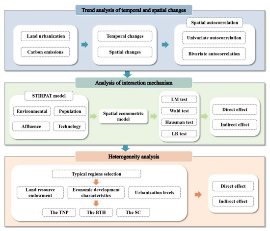
Figure 1.
Research content frame diagram.
2. Analysis Framework
LU is a critical component of the urbanization process, characterized by the expansion of urban built-up areas and a continuous increase in urban construction land. Given the mobility of factors among cities and the spatial interdependence of CEs, theoretically, the impact of LU on CEs includes both direct effects and indirect effects. The direct effect reflects the influence of LU within a local region on CEs in the same region. The indirect effect, also referred to as the spatial spillover effect, represents the impact of LU in one region on the CEs of adjacent regions. Figure 2 is the mechanism analysis diagram.
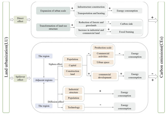
Figure 2.
Mechanism analysis diagram.
2.1. Direct Effect
During the process of LU, the urban built-up area continues to expand, land use and cover undergo persistent changes, and the proportion of urban construction land steadily increases [52]. The continuous increase in industrial and commercial construction land is primarily derived from the conversion of farmland, forest land, and grassland around cities, which serve as important carbon sinks. As land use and cover change progresses, LU results in an increase in carbon sources and a reduction in carbon sinks, thereby exacerbating CEs [36]. On the other hand, the gradual expansion of urban built-up areas leads to increased energy consumption for the needs of transportation and heating, thereby leading to a higher level of CEs [53]. Meanwhile, the expansion of urban space necessitates extensive infrastructure development, including roads, bridges, and buildings, thereby leading to a significant increase in energy consumption. The construction process consumes large quantities of materials such as cement and steel, and the production of these materials is associated with high CEs. Additionally, the expansion of the industrial scale results in substantial CEs due to the combustion of fossil fuels during industrial production processes. Therefore, theoretically, LU is likely to result in an increase in regional CEs.
2.2. Indirect Spillover Effect
According to the First Law of Geography, geographical features and attributes exhibit spatial correlation. Specifically, the closer the geographical proximity between two areas, the stronger their connection [54]. In the dynamic process of regional development, the accelerated LU in one region may exert both a siphon effect and a diffusion effect on adjacent areas [55]. With the progression of LU in this region, urban infrastructure has been continuously improved, the quality of public services has significantly enhanced, employment opportunities have steadily increased, and the agglomeration effect of industrial development has become increasingly prominent. As a result, this process has exerted a strong attraction on population, capital, and various production factors from adjacent regions. Owing to the substantial loss of these factors, the economic development of adjacent regions, particularly in urban space, has been restricted by the total quantity constraint on urban construction land indicators in China. The contraction in industrial production scale, the decline in commercial activities, and the reduction in residents’ living demands are likely to result in a significant decrease in energy consumption and CEs. Furthermore, as this region increasingly attracts population and capital, the income levels of its residents are likely to rise, thereby enhancing the demand for goods and services. This elevated demand, through market linkages and supply chain integration, may indirectly stimulate commercial development in adjacent areas, ultimately leading to increased energy consumption and CEs. However, with the continuous advancement of urbanization, the diffusion effect among regions may also emerge. When a city’s population and development space reach saturation, it tends to diffuse its lower-end industrial models to surrounding regions, potentially leading to increased CEs. Simultaneously, cities with a higher degree of urbanization may also transfer advanced energy technologies to neighboring areas, resulting in a modest reduction in CEs. Given the differing development orientations and stages among cities, the indirect effects between LU and CEs can be either positive or negative.
3. Materials and Methods
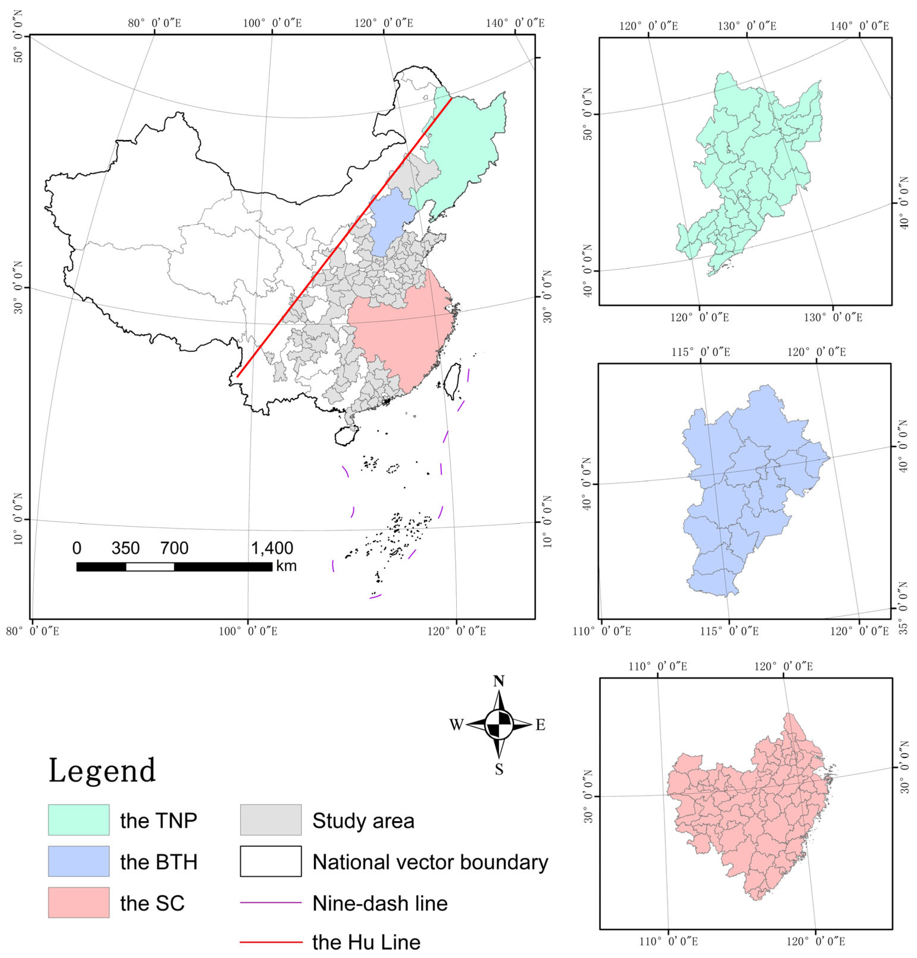
3.1. Study Areas Selection
Given that this study primarily investigates the mechanism by which LU impacts CEs, it is particularly significant to focus on urban areas with a higher degree of urbanization. The Hu Line stretches diagonally from Tengchong in Yunnan Province to Heihe (Aihui) in Heilongjiang Province at a 45-degree angle [56]. The eastern area of the Hu Line demonstrates remarkable development and falls within the category of highly urbanized regions, whereas the urbanization level in the western area is comparatively lower [57]. Notably, CEs associated with construction land in the region east of the Hu Line are significantly higher than those in the western region [58]. Consequently, it is crucial to examine the influence of LU in the eastern region on CEs. Among the cities divided by the Hu Line, those with eastern regions comprising more than half of their total area were retained. The retained city boundaries remain intact, ensuring the validity and reliability of the empirical analysis results. There are a total of 292 prefecture-level cities in the east of the Hu Line. Owing to challenges in acquiring continuous carbon emission data for certain cities, this study ultimately selected 209 prefecture-level cities as the research area (Figure 3). Furthermore, the TNP, the BTH, and the SC will be selected for in-depth comparative analysis. These three regions, located in the northeast, central, and southeast of China, are representative in terms of land resource endowment, regional economic development characteristics, and urbanization levels. The TNP, which is dominated by heavy industry, has faced significant challenges in industrial transformation in recent years but retains ample potential for urban expansion. The BTH focuses on high-tech innovation and high-end service industries, demonstrating a robust trend of industrial synergy within the region, while urban expansion is subject to stringent planning controls. The SC has witnessed rapid growth in manufacturing and modern service industries, such as finance and trade; however, its urban expansion is constrained by limited available space. Consequently, the impact of LU on CEs varies across regions with distinct characteristics. The three regions comprise 35, 13, and 75 prefecture-level cities, respectively, accounting for 45.5% of the total number of prefecture-level cities in the east of the Hu Line. Moreover, their combined GDP constitutes 65% of the total GDP in this region.
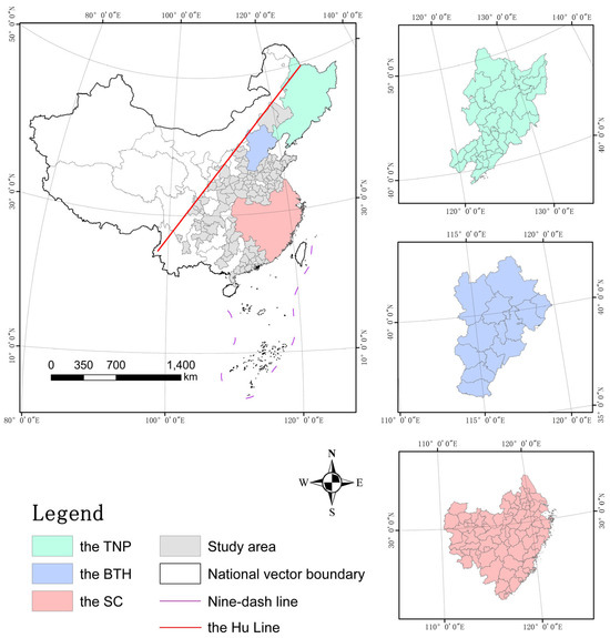
Figure 3.
Location of study area.
The TNP serves as a significant former industrial base in China; however, its overall economic growth rate remains relatively modest, trailing behind the national average [59]. This study excludes the Greater Khingan Mountains region, as it lies west of the Hu Line. In 2019, the average urban GDP of the TNP was 0.14 trillion yuan. The secondary industry accounted for approximately 34.4% of the total output value, while the tertiary industry contributed about 54.6% of the total. The BTH, often referred to as the ‘capital economic circle’ in China [60], boasts excellent resource conditions in terms of urbanization development, economic scale, scientific and technological innovation, and talent resources [61]. In 2019, the BTH had an average urban GDP of 0.65 trillion yuan. The secondary industry contributed approximately 28.7% to the total output value, while the tertiary industry contributed approximately 66.8%. The SC of this study encompasses the Yangtze River Delta urban agglomeration, the middle reaches of the Yangtze River urban agglomeration, and the Guangdong–Fujian–Zhejiang coastal urban agglomeration, which is characterized by a superior geographical location, abundant resources, and high-quality economic development. In 2019, the SC recorded an average urban GDP of 0.63 trillion yuan. The secondary industry accounted for approximately 38.14% of the total output value, while the tertiary industry comprised approximately 51.76% of the total.
3.2. Model Methods
3.2.1. STIRPAT Model
The original IPAT model, which later evolved into the STIRPAT model [62], was initially employed to assess the environmental impact of economic and social development [63]. The environmental impact (I) is determined by a three-variable multiplicative function, namely population (P), affluence (A), and technology (T) [64]. Subsequently, the IPAT model was refined by scholars [65], leading to the development of the STIRPAT model. This model enables a specific decomposition of the influencing factors of population, technology, and affluence, and provides the possibility of specifically studying the impact of a factor with regard to the environment [41]. The STIRPAT model takes the following basic form:
where I represents the environmental impact; P denotes population; A signifies affluence; T represents the technology; α, b, c, and d are parameters to be estimated; and e indicates the random error term.
To address the heteroscedasticity in the STIRPAT model, which refers to the varying variance of the error term, certain adjustments are necessary. Typically, logarithmic transformations are applied to either side of the model. The logarithmic transformation of the STIRPAT model, characterized by its flexibility, allows for the inclusion of multiple additional factors [63]. An effective and widely used method for the quantitative analysis of anthropogenic environmental pressures is the logarithmic transformation of the STIRPAT model. This approach is commonly applied in studies of ecological footprints, energy footprints, and CEs:
Among these variables, CEs represents carbon emissions (unit, ×106 t); LU denotes the ratio of urban built-up area to administrative area (unit, %) [66]; P indicates population size, expressed as the total population in the administrative district (unit, ×104 people) [63]; GDP stands for gross domestic product per capita (unit, yuan) [66]; PTI, or technical level, is defined as the proportion of the value added of the tertiary industry to that of the secondary industry [67].
3.2.2. Spatial Autocorrelation
Typically, the initial stage of spatial econometric analysis involves assessing the spatial autocorrelation of the explanatory variables using Moran’s I index. If significant spatial autocorrelation is detected, it suggests that spatial econometric models can be constructed on this basis. In this study, the spatial autocorrelation method was employed to examine the spatial correlation between LU and CEs from 2010 to 2019. The Moran’s I statistics are as follows:
where: = , represents the CEs of prefecture-level city i; n is the number of cities; is the spatial weights matrix. Moran’s I ranges from −1 to 1. Moran’s I is closer to 1 when there is a higher positive spatial correlation between cities, and closer to −1 when there is a greater negative spatial correlation. When the value is close to 0, it indicates that the spatial distribution is random rather than exhibiting spatial autocorrelation across regions [68]. In this study, three types of spatial weights were selected to test the spatial interaction relationships: adjacency weight (W1), geographical distance weight (W2), and economic distance weight (W3).
3.2.3. Bivariate Spatial Autocorrelation
Bivariate spatial autocorrelation can reflect the spatial agglomeration relationship between two different attribute variables. The global bivariate Moran’s I was used to study the spatial correlation and degree between LU and CEs, while the local bivariate Moran’s I was used to study the spatial correlation between LU and CEs in the unit region. The calculation formula is as follows:
where I and are global bivariate Moran’s I and local bivariate Moran’s I, respectively; n is the number of cities; is the spatial weight matrix; and are the attribute values of cities i and j, respectively; and and are the mean and variance of the attribute values.
3.2.4. Spatial Econometric Model
In this study, panel data approaches are integrated with spatial econometric techniques through the application of spatial econometric models. Compared to the classic model, the spatial econometric model pioneers the simultaneous incorporation of spatio-temporal elements into the system of study, thereby enhancing the accuracy of estimation results [69]. Therefore, the spatial econometric model was constructed based on the STIRPAT model:
where i and j indicate different cities; indicates spatial weights; indicates explanatory variables; indicates CEs in city i; indicates CEs in city j; β represents the regression coefficient of the explanatory variables; ρ denotes the spatial regression coefficient of the explained variables; φ indicates the spatial regression coefficient of the explanatory variables; λ indicates the spatial error regression coefficient. If ρ ≠ 0, φ = 0 and λ = 0, then the equation is the spatial lag model (SLM); if ρ = 0, φ = 0 and λ ≠ 0, then the equation is the spatial error model (SEM); if ρ ≠ 0, φ ≠ 0 and λ = 0, then the equation is the spatial Durbin model (SDM).
3.3. Data Source and Processing
The China Emission Accounts and Datasets (CEADs) (https://ceads.net/ (accessed on 1 January 2024)) was utilized as the source for urban CEs data. Population, per capita GDP, and the added value of the secondary and tertiary industries were derived from the China Urban Statistical Yearbook [70], whereas urban built-up area and administrative area data were obtained from the China Urban Construction Statistical Yearbook [71]. Linear interpolation was applied to supplement missing values in each dataset.
4. Results
4.1. Spatial and Temporal Changes of LU and CEs
4.1.1. Spatial and Temporal Changes of LU
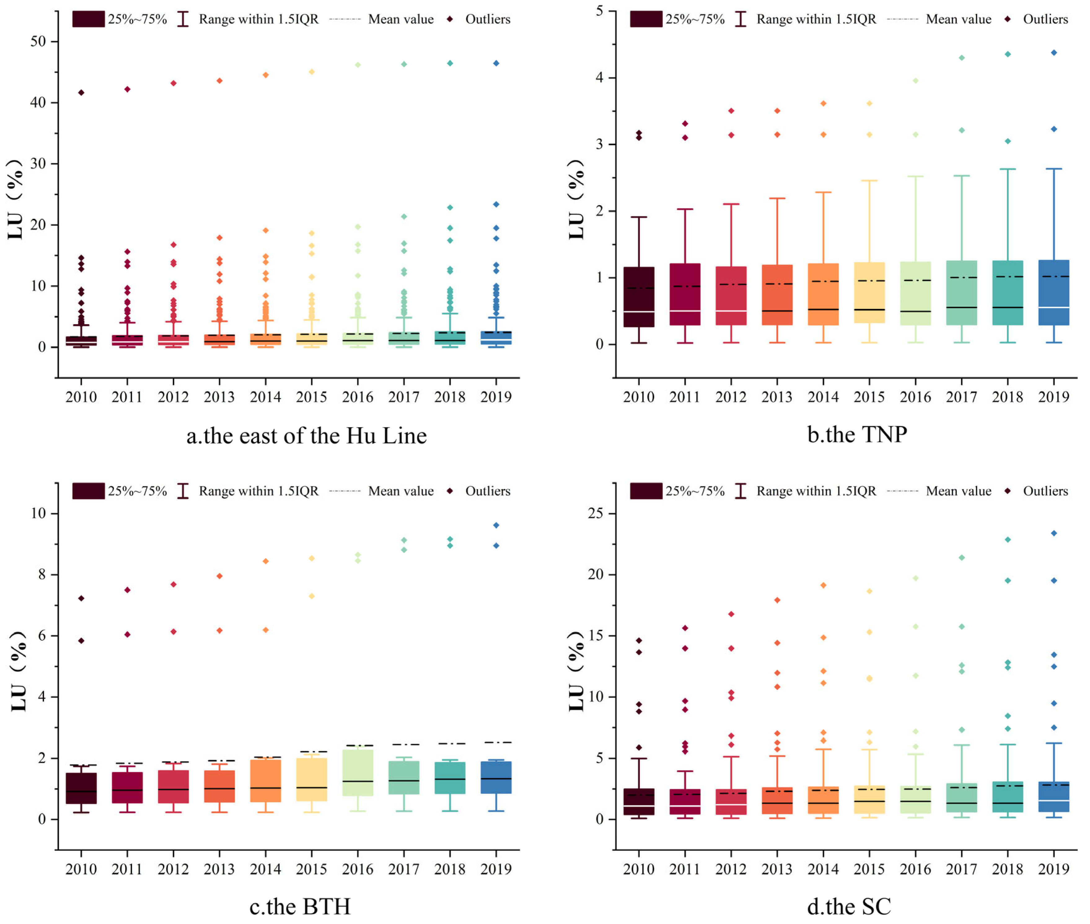
The temporal trend of LU from 2010 to 2019 is depicted in the box plots presented in Figure 4. The mean value of LU in the east of the Hu Line increased from 1.711% to 2.435%, corresponding to an average annual growth rate of 4.3%. The mean value of LU in the total TNP increased from 0.847% to 1.021%, with an average annual growth rate of 2.1% and minimal variation. The mean value of LU increased from 1.780% to 2.522% in the BTH and from 1.996% to 2.834% in the SC. Despite the relatively low mean value of LU, the presence of outliers indicated that LU values range from 5% to 50% in some cities, mostly located in the BTH and the SC.
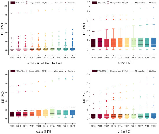
Figure 4.
Temporal trend of LU ((a) the east of the Hu Line; (b) the TNP; (c) the BTH; (d) the SC).
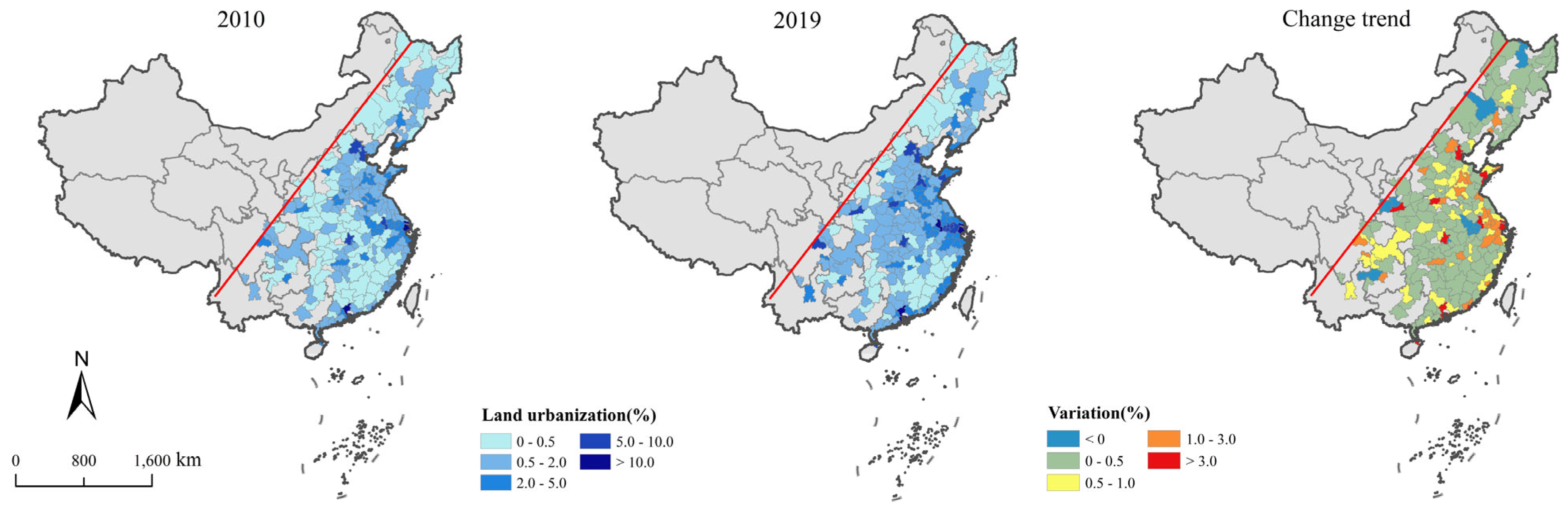
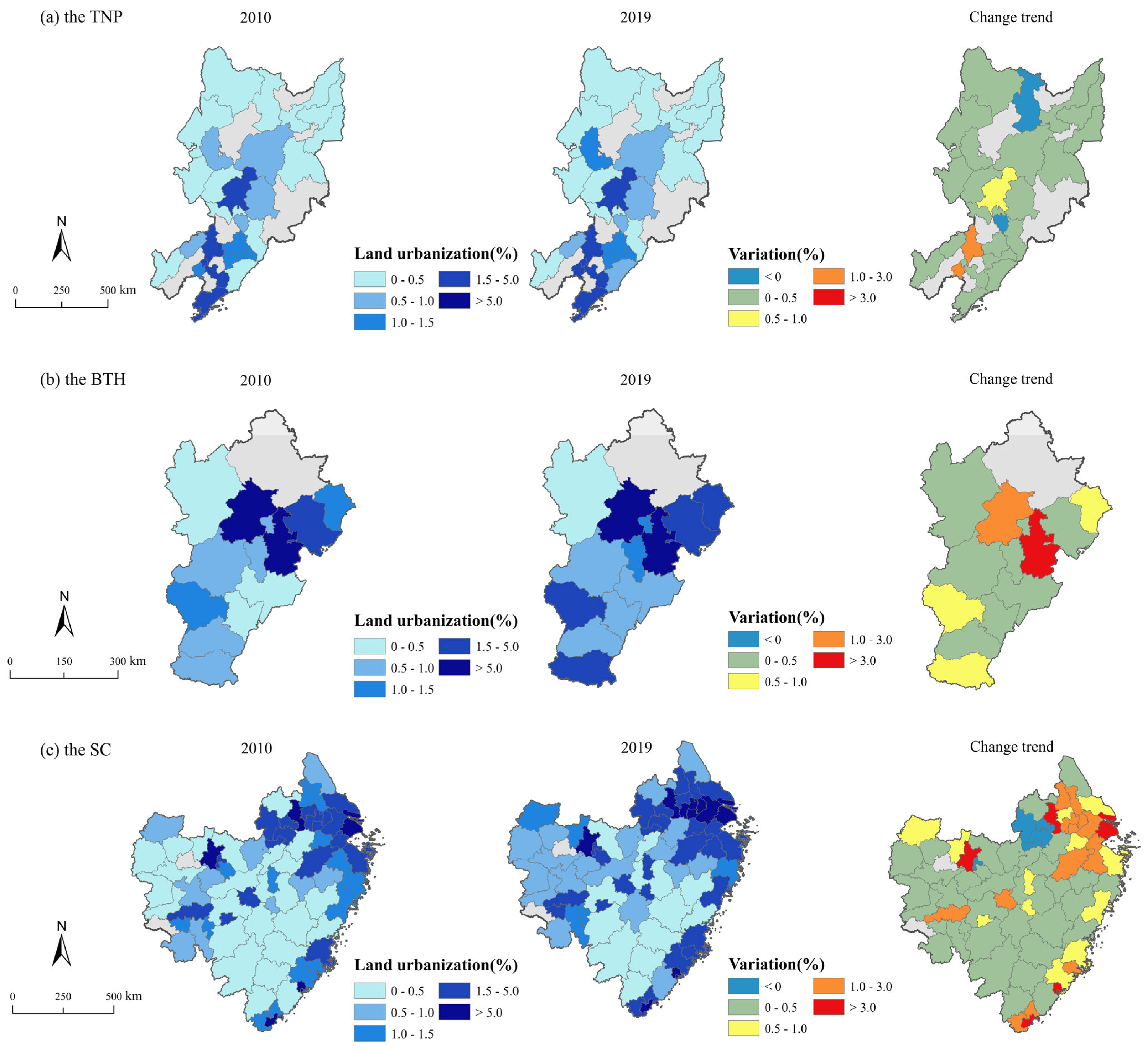
LU values exhibit a spatial distribution pattern characterized by higher levels in the central regions and lower levels in the northern and southern regions from 2010 to 2019 (Figure 5). Only 11 cities experienced a decline in LU, primarily concentrated in the Northeast area. LU exhibits a distribution pattern characterized by high values in central cities that radiate outward to surrounding areas in the TNP and the BTH (Figure 6). In contrast, in the SC, LU demonstrates a spatial distribution trend of gradually decreasing from the eastern coastal areas to the western inland areas. The areas with a decline in LU in the TNP include Yichun and Liaoyuan City. In the BTH, Beijing and Tianjin, both municipalities directly under the Central Government, serve as high-value centers for LU, while the remaining areas experience a slight increase trend. The growth rate of LU in coastal cities has been significantly accelerated, forming a distinct high-value concentration zone.

Figure 5.
Distribution of LU in the east of the Hu Line.
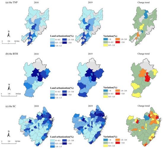
Figure 6.
Distribution of LU in three regions ((a) the TNP; (b) the BTH; (c) the SC).
4.1.2. Spatial and Temporal Changes of CEs
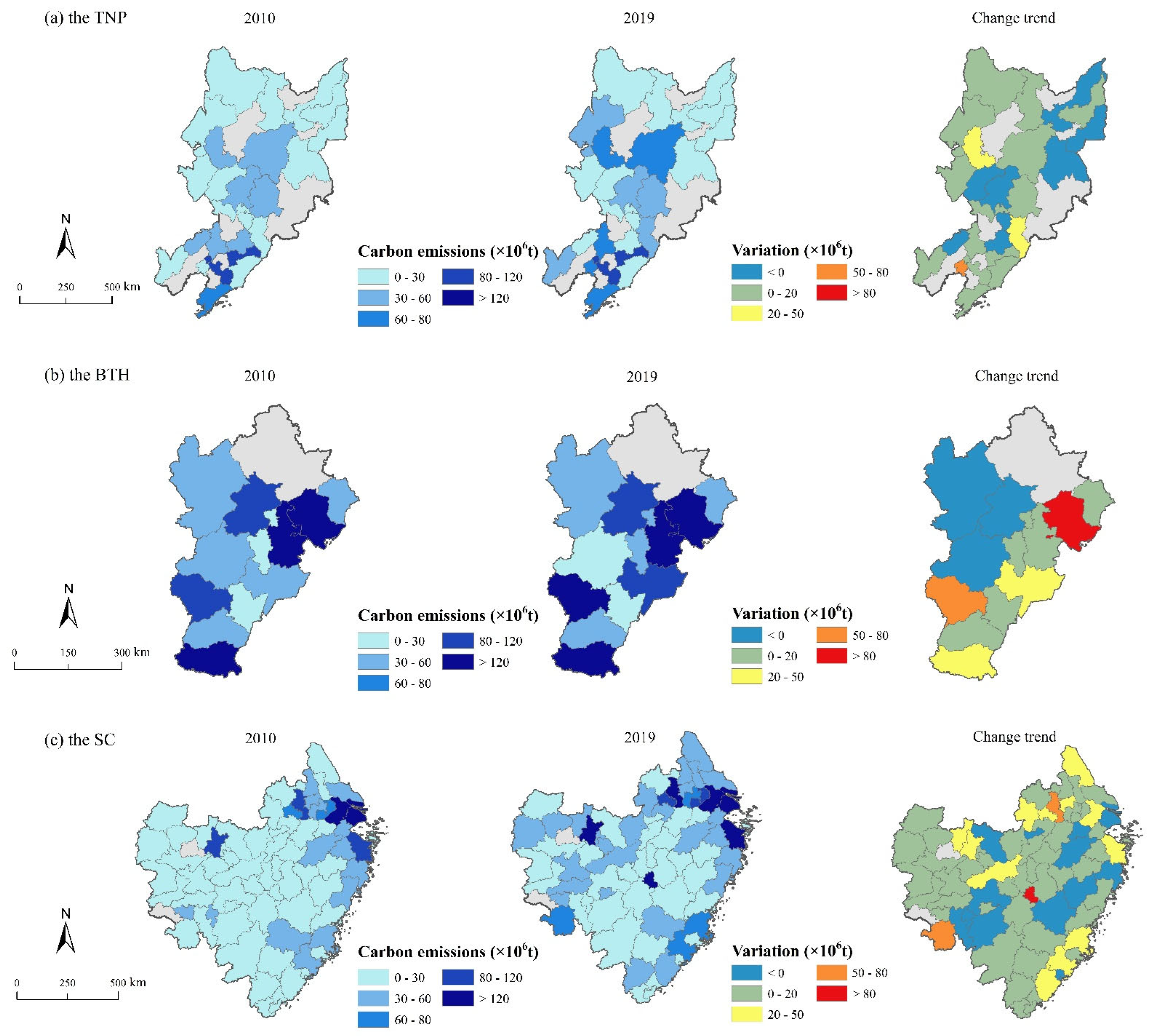
The mean value of CEs in the east of the Hu line increased from 35 × 106 t to 48 × 106 t from 2010 to 2019, with an average annual increase of 3.5% (Figure 7). In the BTH, CEs is significantly higher than that of the other two regions. Over the study period, it exhibited a trend of fluctuation and increase. In 2015, it slightly declined to 80.4 × 10⁶ t, and reached its peak again in 2019, standing at 108 × 106 t. By contrast, in the TNP and the SC, CEs showed relatively gentle growth trends and both reached high values in 2019, at 38.1 × 10⁶ t and 45.3 × 10⁶ t, respectively.
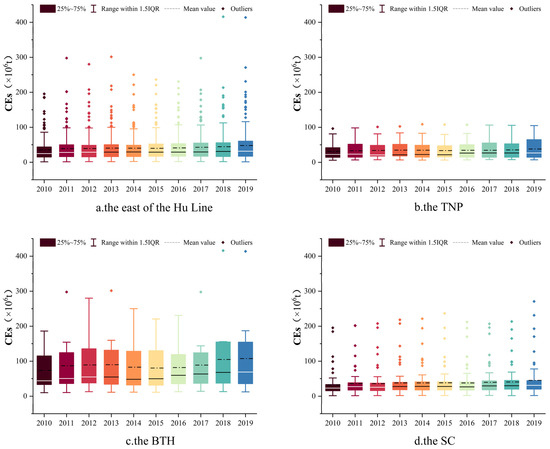
Figure 7.
Temporal trend of CEs ((a) the east of the Hu Line; (b) the TNP; (c) the BTH; (d) the SC).
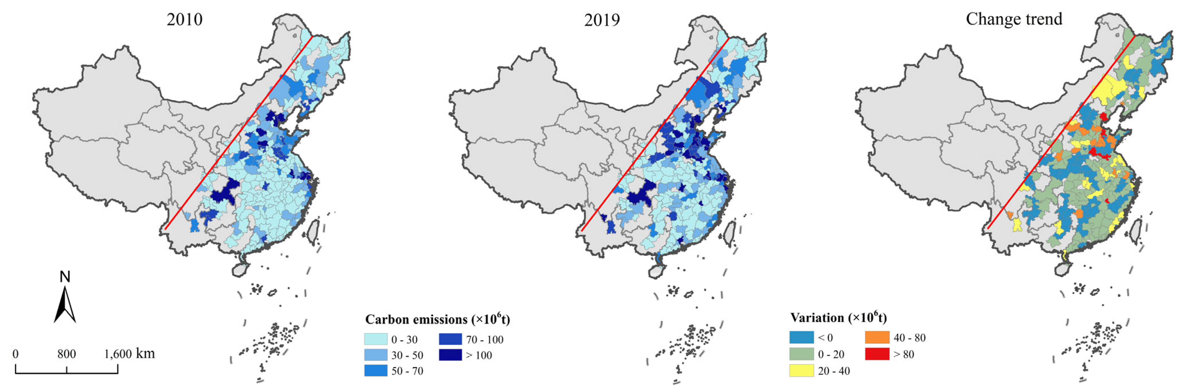
From 2010 to 2019, 70.3% of the cities within the study area exhibited an upward trend in CEs (Figure 8). Conversely, 29.7% of the cities experienced a decline in CEs, with these reductions primarily observed in the SC and the TNP, including major urban centers such as Shanghai, Hangzhou, and Xiamen. In the TNP, areas with high CEs are relatively scarce, mainly distributed in the southern part of Liaoning Province, while CEs in Jilin and Heilongjiang Provinces are relatively low (Figure 9). Moreover, 32% of the cities in the TNP show a trend toward negative growth. In the BTH, several cities have experienced a decline in CEs, particularly in Beijing and its surrounding areas. In the SC, high-value carbon emission areas are predominantly located in the northern and eastern coastal zones. Approximately 18.3% of cities demonstrate a decreasing trend, mainly distributed across Zhejiang and Jiangxi provinces.
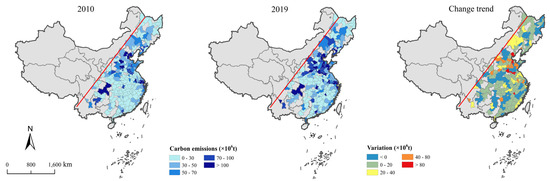
Figure 8.
Distribution of CEs in the east of the Hu Line.
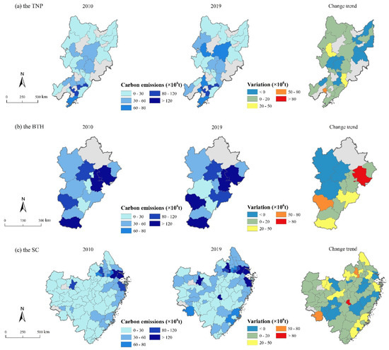
Figure 9.
Distribution of CEs in three regions ((a) the TNP; (b) the BTH; (c) the SC).
4.2. Empirical Results and Analysis
4.2.1. Spatial Autocorrelation Analysis
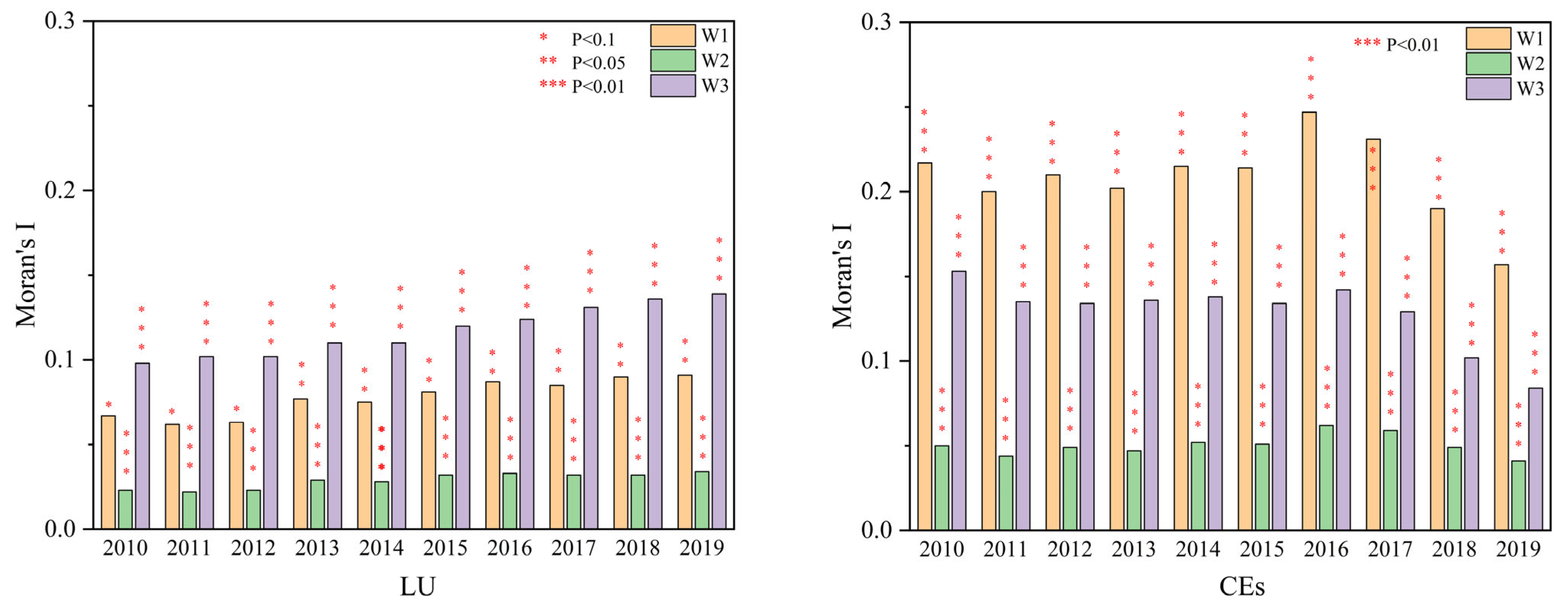
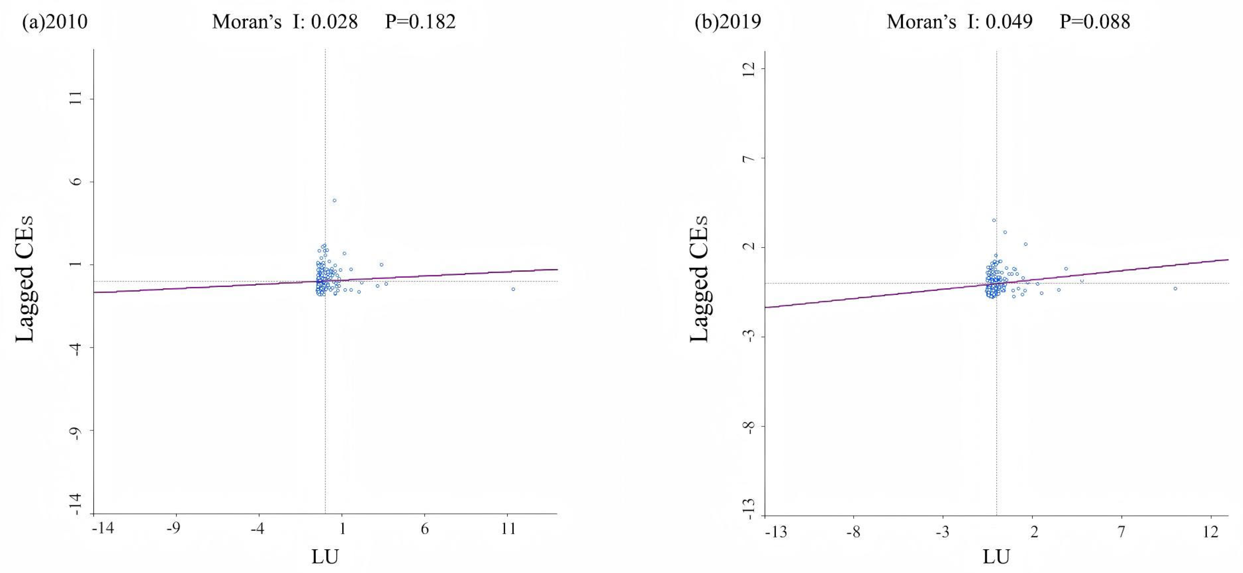
Figure 10 demonstrates that Moran’s I of LU and CEs under the three weight matrices is statistically significant, with positive coefficients. This suggests a pronounced positive spatial correlation for both LU and CEs, where the Moran’s I of CEs significantly exceeds that of LU. Figure 11 presents the bivariate Moran’s I scatter plot between LU and CEs, showing no statistically significant p-value in 2010, while a significant p-value (0.049) was identified in 2019. Therefore, it is necessary to apply spatial econometric models to further examine the spatial relationship.
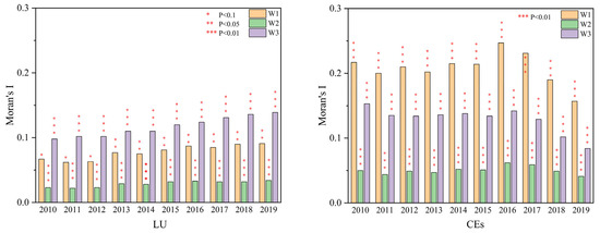
Figure 10.
Moran’s I of the three weight matrices.
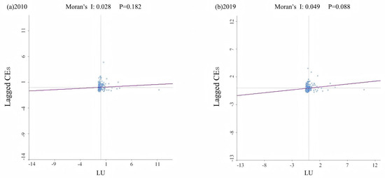
Figure 11.
The bivariate Moran’s I scatter plot of LU and CEs ((a) 2010; (b) 2019).
4.2.2. LISA Cluster Analysis
Figure 12 illustrates the comprehensive bivariate LISA aggregation diagram between LU and CEs in 2010 and 2019. During the study period, the number of cities exhibiting a significant interaction relationship between LU and CEs steadily increased, primarily characterized by Low–Low clusters and High–High clusters. High–High clusters are predominantly located in the BTH and the northeastern regions of the SC, with a notable increase observed in the eastern region. Low–Low clusters account for a substantial proportion and are mainly distributed across the SC. Low–High clusters are predominantly situated in the central region, displaying characteristics of surrounding High–High clusters and showing a significant increase. The proportion of High–Low clusters is relatively small, with these clusters primarily located in Wuhan and Nanchang within the SC and Chengdu.
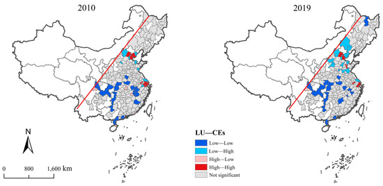
Figure 12.
Bivariate LISA cluster between LU and CEs in the east of the Hu Line.
4.2.3. Empirical Analysis of the Impact of LU on CEs
(1) Model Selection Results
The LM test and R-LM test are utilized to determine the appropriate spatial econometric model. The Wald test and LR test evaluate whether the SDM model can be simplified into a less complex form. If the Hausman test is statistically significant, the fixed-effect model is preferred; otherwise, the random-effect model is selected [63]. As presented in Table 1, the LM tests for both the spatial error model and the spatial lag model under W1 are significant at the 1% and 5% levels, while the R-LM tests are significant at the 1% level. Additionally, both the Wald test and LR test passed the 1% significance level. The LM test and R-LM test for the spatial error model under W2 are significant at the 1% level. The LM test and R-LM test for the spatial lag model under W3 are significant at the 1% level. The time effect results of the Hausman test and LR test under the three weight matrices are all significant at the 1% level. Therefore, the time-fixed effect spatial Durbin model, time-fixed effect spatial error model, and time-fixed effect spatial lag model are employed to analyze the three weight matrices, respectively.

Table 1.
Model test results under three weight matrices.
(2) Spatial econometric regression results
The empirical results presented in Table 2 reveal that the coefficients of LU (lnLU) are positive and statistically significant at the 1% level across all three weight matrices, with the highest coefficient of 0.145 observed under adjacent weights. This suggests that LU has a statistically significant promoting effect on CEs, aligning with theoretical analysis of a positive direct relationship between LU and CEs. The coefficient of W_ lnLU is significantly negative at the 1% statistical level, indicating that LU exerts a negative spatial spillover effect on CEs. Specifically, an increase in LU within this region is likely to result in a reduction of CEs in adjacent regions. For other variables, the coefficients of economic level (lnGDP) and population size (lnP) are also positive and significant at the 1% level, consistent with prior research findings [63]. In contrast, the coefficient for technical level (lnPTI) is negative and significant at the 1% level, supporting the conclusion drawn by Bai et al. [72] that technological progress can effectively mitigate CEs. Notably, LU has the most limited influence on CEs compared to other factors. Population growth and economic development remain the primary drivers of carbon emissions, while technological advancements have played a crucial role in mitigating carbon emission intensity.
Table 2.
Spatial econometric model estimation results.
(3) Decomposition of Spatial Spillover Effects
LeSage and Pace [73] contended that, owing to the spatial lag term of variables in the spatial Durbin model, the estimated coefficients cannot directly reflect the magnitude of influence of the independent variables on the dependent variable. Instead, these coefficients merely provide information regarding the direction and significance level. Consequently, to adequately evaluate the impact of independent variables on dependent variables, the model must incorporate additional estimates of the direct, indirect, and total effects.
Based on the findings presented in Table 3 for W1, it is evident that, from the perspective of LU, the direct effect coefficient is positive and significant at the 1% level. This suggests that for every 1% increase in LU within the region, CEs increase by 0.129%. Furthermore, the indirect effect coefficient is negative and significant at the 1% level, indicating a negative spillover effect. For every 1% increase in LU within the region, CEs in adjacent regions decrease by 0.224%. This result highlights the pronounced polarization effect and siphoning effect of LU on surrounding regions. The rapid expansion of urban areas has resulted in resource deprivation in neighboring cities, thereby contributing to a marginal reduction in CEs.
Table 3.
Results of direct and indirect effects.
The direct effect coefficient of the economic level is positive and significant at the 1% level. Specifically, for every 1% increase in economic growth, CEs increase by 0.564%. This interaction can be attributed to the fact that economic growth continues to rely on substantial energy consumption, which comes at the expense of environmental degradation and is accompanied by a marginal increase in CEs. Furthermore, the indirect effect coefficient is also positive and statistically significant at the 1% level, indicating a positive spillover effect of the economic level on CEs in adjacent regions. For each 1% increase in economic growth, CEs in adjacent regions increase by 0.480%. This phenomenon can be attributed to the region’s economic growth driving the economic expansion of adjacent regions, which leads to substantial energy consumption and subsequently promotes CEs.
The direct effect coefficient of the technical level is negative and significant at the 1% level. Specifically, for every 1% increase in technical level, CEs decrease directly by 0.365%. This interaction can be attributed to the emphasis on resource efficiency and emission abatement policies in China, where the development of green production technologies and other innovations has enhanced energy use efficiency, thereby reducing energy consumption and inhibiting CEs. Additionally, the indirect effect coefficient is positive and statistically significant at the 1% level, indicating a positive spillover effect of the technical level on CEs in adjacent regions. Specifically, for every 1% increase in technical level, CEs increase by 0.538% in adjacent regions. This phenomenon can be attributed to the fact that technological progress has not yet fully diffused to the surrounding areas, creating a technological gap in those areas. Consequently, the relatively slower technological development in adjacent regions leads to reduced energy efficiency and increased energy demand, which promotes higher CEs.
The direct effect coefficient of population size is positive and statistically significant at the 1% level. Specifically, for every 1% increase in population, CEs increase by 0.695% directly. This phenomenon can be attributed to the growth in population, which leads to increased transportation demand, and higher energy consumption for residential heating, and other living-related energy uses, thereby promoting the generation of CEs. However, the indirect effect is not statistically significant.
4.2.4. Regional Heterogeneity Analysis of LU on CEs
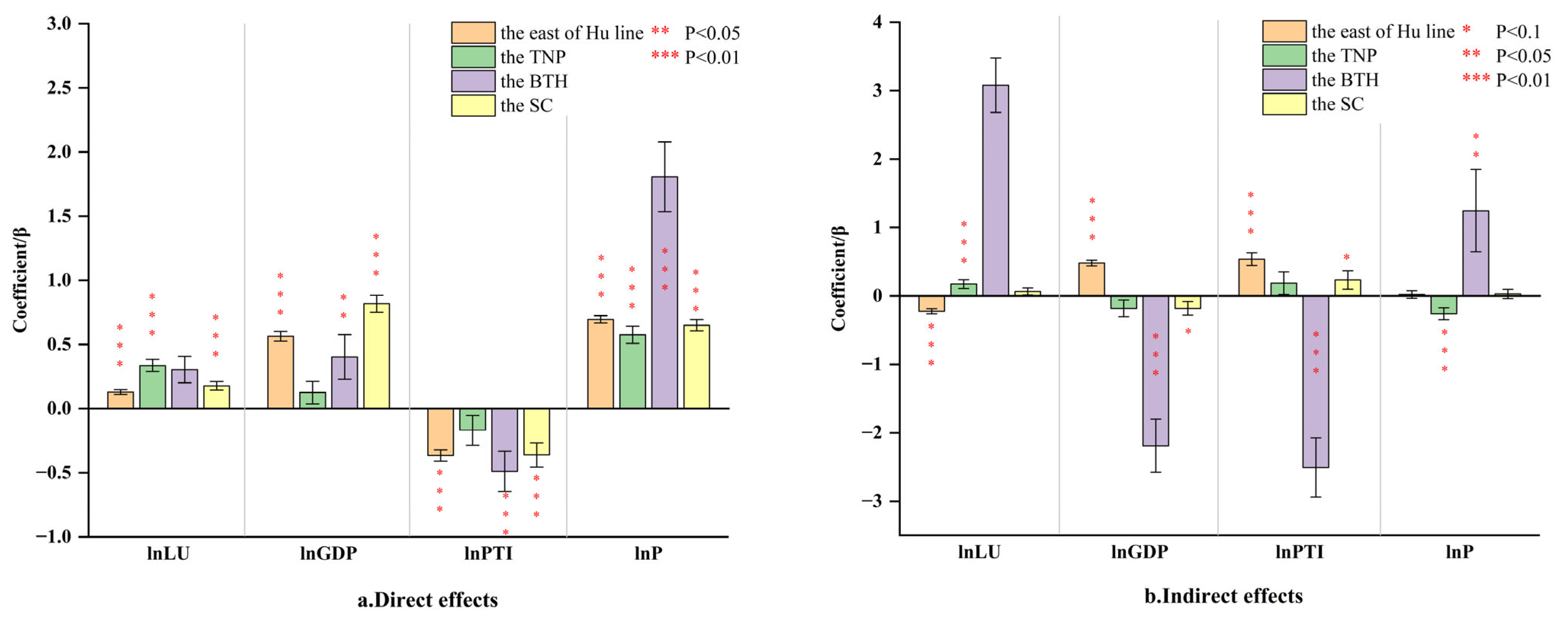
Through the spatial econometric analysis, it is evident that the impact of LU on CEs exhibits significant regional disparities (Figure 13). For detailed results, please refer to Appendix A. Whether considering the direct effect or the indirect effect, the level of LU in the TNP is significantly positive. Specifically, the direct effect coefficient is 0.336 and statistically significant at the 1% level, while the indirect effect coefficient, slightly smaller than the direct effect, is 0.174 and also statistically significant at the 1% level. In the SC, the direct effect of LU on CEs is significant, while the indirect effect coefficient is not significant. The direct effect coefficient is 0.177, which is significant at the statistical level of 1%. It is worth noting that in the BTH, the impact of LU on CEs is not significant either directly or indirectly.

Figure 13.
Decomposition of spatial effects ((a) Direct effects; (b) Indirect effects).
The varying results of the direct effects across the three regions suggest that LU is one of the core driving forces for the development of the TNP and also a critical factor contributing to the increase in regional CEs. These findings can likely be attributed to the relatively low level of LU within the TNP, as confirmed by the earlier spatio-temporal analysis, which provides substantial room for urban expansion. Consequently, the industrial development structure in this region remains relatively reliant on land resources and energy consumption. In contrast, in the SC, the positive impact of LU on regional CEs remains significantly positive but with lower intensity compared to the TNP. Furthermore, its influence is weaker than the effects of economic growth and population increase, indicating that urban expansion is no longer the primary driver of development in the SC. Additionally, in the BTH, the statistically insignificant results imply that the expansion of urban construction land is no longer a dominant driver of CEs. This conclusion is further supported by the spatio-temporal analysis, which reveals that LU and CEs have become decoupled in some major cities within the BTH.
The varying results of indirect effects in the three regions reveal the interaction patterns of land factors and regional disparities in land resource endowment. In the TNP, the positive spatial spillover effect can be attributed to the relatively abundant land development planning indicators and ample development space, which fosters an emulation effect of “development reliant on urban land resources” among regions. Consequently, this leads to the proliferation of inefficient industrial development models across regions, thereby increasing carbon emission intensity. However, the indirect effect is not significant in the SC and the BTH, which further indicates that the development mode of inter-regional urban construction land expansion is difficult to sustain due to the scarcity of urban land resources.
Further analysis of the measurement results reveals that, despite the insignificant level of LU in the BTH, economic growth, technological progress, and population growth remain key factors significantly influencing CEs. In particular, population growth has the most substantial impact on CEs, with direct and indirect effect coefficients of 1.807 and 1.241, respectively, both significant at the 1% and 5% levels. This phenomenon is also observed in the TNP and the SC, indicating that population factors are still the primary factor affecting regional CEs at this stage. The influence of technological progress exhibits significant variation across the three regions. In the TNP, neither the direct nor the indirect effects of technological progress are significant, suggesting that technological progress has yet to become a core driver of regional development and consequently has a limited impact on environmental improvement. In contrast, in the SC and the BTH, the direct effects of technological progress are statistically significant, indicating that technological advancements have facilitated transformations in energy and industrial structures, leading to positive environmental impacts. Notably, in the BTH, the indirect effect of technological progress is −2.509 and statistically significant at the 1% level, suggesting that technological progress has generated a diffusion effect, positively influencing surrounding areas environmentally.
5. Discussion
5.1. Summary of Findings
Spatial econometric analysis demonstrates that LU is indeed one of the key factors influencing CEs in the east of the Hu Line at the current stage. The rapid expansion of urban areas has led to an increase in local carbon emission intensity. Regional spatial planning policies in China aim to coordinate development, environmental protection, and resource efficiency across space. The core frameworks include the Territorial Spatial Planning System [74], the Main Functional Zoning Strategy [75], and New-Type Urbanization Plans [76], which collectively promote differentiated development paths. However, constrained by regional spatial planning policies that restrict urban scale, the development of surrounding cities is currently influenced by spatial polarization effects. As a result, LU has generated an overall negative spatial spillover effect. This finding is consistent with the results reported in previous studies [77]. Even in the eastern area of the Hu Line, which generally exhibits higher levels of urbanization, the heterogeneity among different regions remains pronounced. This heterogeneity is a key reason for the varied conclusions in previous studies [36,41,62,77,78], and the differential results of the heterogeneity analysis in this study further substantiate this viewpoint. The differentiated interactions between LU and CEs in these regions are closely linked to their developmental stages and regional characteristics.
The development model centered on urban expansion as a driver of economic growth exhibits distinctive features in China, serving as a crucial impetus for the country’s rapid and leapfrogging economic advancement following the reform and opening-up policy. However, this model may have adverse effects on environmental protection and green development, thereby constraining urban high-quality development to some extent. In response to these challenges, the Chinese government has formulated comprehensive strategies under the New-Type Urbanization Initiative, implementing territorial spatial planning to enhance regional governance frameworks and promote the low-carbon transformation of urban spatial configurations. The decarbonization of urban spatial development is expected to become the dominant trend in future development paradigms.
5.2. Limitation and Future Outlook
The selection of data and years in this study is subject to certain limitations, which may affect the comprehensiveness and generalizability of the findings. The research year was not updated to the latest year, and the spatial changes and internal mechanisms of LU and CEs in recent years were not analyzed. In recent years, when data availability is limited, LU may contribute to advancements in the technology sector. For example, the emergence of green building projects and the development of eco-industrial parks in cities have often been associated with reductions in CEs due to changes in land use. However, outdated data fail to capture these developments, leading to potential biases in assessing the actual trends of CEs during LU. Consequently, this could result in an underestimation of the positive contributions of LU to energy conservation and emission reduction. In future studies, the impact of county-scale LU on CEs will be thoroughly explored using up-to-date data.
5.3. Policy Suggestions
The research findings lead this study to suggest the following policy measures, which aim to comprehensively consider regional differences and sustainable development goals, thereby providing guidance for China in formulating carbon emission reduction policies and urbanization strategies.
(1) Control urban expansion: Local governments should carefully regulate the scale and spatial extent of urban development through scientific territorial spatial planning. Limiting the increase of urban construction land can play a key role in achieving regional carbon targets.
(2) Tailor region-specific strategies: Given the differences in urban development and LU impact, differentiated strategies are essential. For the TNP and the SC, optimizing land use and curbing excessive expansion are crucial. In the BTH, promoting urban quality through technological innovation and industrial upgrading should take priority.
(3) Strengthen policy coordination: Governments should promote cross-sectoral collaboration in land use, environmental protection, and energy policy. Harmonized planning and integrated governance are critical to aligning LU with low-carbon development goals.
6. Conclusions
This study investigates the impact mechanism of LU on CEs in 209 cities located east of the Hu Line in China. Using spatial econometric models based on the STIRPAT framework, and incorporating spatial spillover effects and regional heterogeneity, several key conclusions are drawn, as follows:
(1) General trends: Between 2010 and 2019, both LU and CEs in the study area exhibited consistent upward trends, with annual growth rates of 4.3% and 3.5%, respectively. Significant positive spatial correlations were observed, and spatial clustering patterns revealed regional disparities: high-value clusters were predominantly concentrated in the BTH and SC, while low-value clusters showed significant concentration within the TNP.
(2) Empirical findings: LU exhibits a statistically significant positive effect on CEs at the 1% significance level, with a direct effect coefficient of 0.129. The indirect effect is characterized by a coefficient of −0.224, indicating that LU in the region exerts a negative spatial spillover effect on CEs in adjacent areas.
(3) Regional heterogeneity: The TNP demonstrates the most pronounced impact of LU on CEs, with direct and indirect effects of 0.336 and 0.174, respectively. In the SC, LU exerts a statistically significant direct effect (0.177) but lacks a notable spillover impact. In contrast, LU has no significant influence on CEs in the BTH, suggesting a decoupling of land expansion and emissions in highly developed regions.
In conclusion, these findings are intended to provide a more comprehensive and actionable framework for the development of national carbon reduction policies. By systematically accounting for regional disparities and strictly adhering to the principles of sustainable development, we can more effectively tackle the challenges posed by climate change and promote a greener, more sustainable future.
Author Contributions
Conceptualization, H.G. and X.C.; methodology, H.S.; software, X.C.; validation, C.H. and B.W.; formal analysis, H.S.; investigation, H.G.; resources, H.G.; data curation, X.C.; writing—original draft preparation, X.C.; writing—review and editing, H.G.; visualization, C.H.; supervision, B.W.; project administration, H.G.; funding acquisition, H.G. All authors have read and agreed to the published version of the manuscript.
Funding
This research was funded by the Ministry of Education Humanities and Social Sciences General Research Project (grant number: 23A10157004), Liaoning Provincial Department of Education, Social Science Project, Study on the Decoupling Relationship between Land Use Efficiency and Carbon Emission and its Realization Path in Three Eastern Provinces in the Context of New Urbanization (grant number: JYTQN2024019), Liaoning Provincial Department of Science and Technology, Qingyuan County Ground Power Enhancement Science and Technology Mission, Liaoning Province (grant number: 2024JH5/10400158), Propaganda Department of Liaoning Provincial Committee of the Communist Party of China, “Xingliao Talent Program” “Cultural Masters” and “Four Batch” Talents (grant number: XLYC2210046).
Data Availability Statement
Dataset available on request from the authors.
Conflicts of Interest
The authors declare no conflicts of interest.
Appendix A
Table A1.
Results of direct and indirect effects in the TNP.
Table A1.
Results of direct and indirect effects in the TNP.
| Variables | Model I W1 | ||
|---|---|---|---|
| Direct Effect | Indirect Effect | Total Effect | |
| lnLU | 0.336 *** | 0.174 *** | 0.510 *** |
| (0.047) | (0.063) | (0.043) | |
| lnGDP | 0.125 | −0.181 | −0.056 |
| (0.087) | (0.122) | (0.110) | |
| lnPTI | −0.169 | 0.187 | 0.017 |
| (0.116) | (0.165) | (0.103) | |
| lnP | 0.576 *** | −0.259 *** | 0.317 *** |
| (0.068) | (0.089) | (0.076) | |
Note: *** indicates significance at the 1% statistical level. Robust standard error in parentheses.
Table A2.
Results of direct and indirect effects in the BTH.
Table A2.
Results of direct and indirect effects in the BTH.
| Variables | Model I W1 | ||
|---|---|---|---|
| Direct Effect | Indirect Effect | Total Effect | |
| lnLU | 0.304 | 3.080 | 3.384 |
| (0.103) | (0.399) | (0.475) | |
| lnGDP | 0.403 ** | −2.190 *** | −1.787 *** |
| (0.174) | (0.387) | (0.462) | |
| lnPTI | −0.489 *** | −2.509 *** | −2.998 *** |
| (0.157) | (0.433) | (0.553) | |
| lnP | 1.807 *** | 1.241 ** | 3.048 *** |
| (0.271) | (0.600) | (0.853) | |
Note: ** and *** indicate significance at the 5%, and 1% statistical levels, respectively. Robust standard error in parentheses.
Table A3.
Results of direct and indirect effects in the SC.
Table A3.
Results of direct and indirect effects in the SC.
| Variables | Model I W1 | ||
|---|---|---|---|
| Direct Effect | Indirect Effect | Total Effect | |
| lnLU | 0.177 *** | 0.067 | 0.244 *** |
| (0.033) | (0.053) | (0.038) | |
| lnGDP | 0.817 *** | −0.181 * | 0.636 *** |
| (0.066) | (0.099) | (0.068) | |
| lnPTI | −0.361 *** | 0.235 * | −0.126 |
| (0.095) | (0.134) | (0.104) | |
| lnP | 0.650 *** | 0.031 | 0.681 *** |
| (0.044) | (0.068) | (0.075) | |
Note: * and *** indicate significance at the 10% and 1% statistical levels, respectively. Robust standard error in parentheses.
References
- Zhang, S.; Li, Z.; Ning, X.; Li, L. Gauging the impacts of urbanization on CO2 emissions from the construction industry: Evidence from China. J. Environ. Manag. 2021, 288, 112440. [Google Scholar] [CrossRef] [PubMed]
- Kahn, M.E.; Mohaddes, K.; Ng, R.N.C.; Pesaran, M.H.; Raissi, M.; Yang, J.-C. Long-term macroeconomic effects of climate change: A cross-country analysis. Energy Econ. 2021, 104, 105624. [Google Scholar] [CrossRef]
- Auffhammer, M.; Carson, R.T. Forecasting the path of China’s CO2 emissions using province-level information. J. Environ. Econ. Manag. 2008, 55, 229–247. [Google Scholar] [CrossRef]
- Fan, M.; He, G.; Zhou, M. The winter choke: Coal-Fired heating, air pollution, and mortality in China. J. Health Econ. 2020, 71, 102316. [Google Scholar] [CrossRef]
- Wang, S.; Fang, C.; Guan, X.; Pang, B.; Ma, H. Urbanisation, energy consumption, and carbon dioxide emissions in China: A panel data analysis of China’s provinces. Appl. Energy 2014, 136, 738–749. [Google Scholar] [CrossRef]
- Li, Z.-Z.; Li, R.Y.M.; Malik, M.Y.; Murshed, M.; Khan, Z.; Umar, M. Determinants of Carbon Emission in China: How Good is Green Investment? Sustain. Prod. Consum. 2021, 27, 392–401. [Google Scholar] [CrossRef]
- Tan, X.; Dong, L.; Chen, D.; Gu, B.; Zeng, Y. China’s regional CO2 emissions reduction potential: A study of Chongqing city. Appl. Energy 2016, 162, 1345–1354. [Google Scholar] [CrossRef]
- Zhao, J.; Jiang, Q.; Dong, X.; Dong, K. Assessing energy poverty and its effect on CO2 emissions: The case of China. Energy Econ. 2021, 97, 105191. [Google Scholar] [CrossRef]
- Yang, S.; Yang, X.; Gao, X.; Zhang, J. Spatial and temporal distribution characteristics of carbon emissions and their drivers in shrinking cities in China: Empirical evidence based on the NPP/VIIRS nighttime lighting index. J. Environ. Manag. 2022, 322, 116082. [Google Scholar] [CrossRef]
- Gu, H.; Ma, T.; Qian, F.; Cai, Y. County land use scenario simulation and carbon emission effect analysis using CLUE-S model. Trans. CSAE 2022, 38, 288–296. [Google Scholar] [CrossRef]
- Wei, M.; Cai, Z.; Song, Y.; Xu, J.; Lu, M. Spatiotemporal evolutionary characteristics and driving forces of carbon emissions in three Chinese urban agglomerations. Sustain. Cities Soc. 2024, 104, 105320. [Google Scholar] [CrossRef]
- Bahrami, S.; Amini, M.H. A Decentralized Trading Algorithm for an Electricity Market with Generation Uncertainty. Appl. Energy 2017, 218, 520–532. [Google Scholar] [CrossRef]
- Du, L.; Hanley, A.; Zhang, N. Environmental technical efficiency, technology gap and shadow price of coal-fuelled power plants in China: A parametric meta-frontier analysis. Resour. Energy Econ. 2016, 43, 14–32. [Google Scholar] [CrossRef]
- Zhou, Y.; Chen, M.; Tang, Z.; Mei, Z. Urbanization, land use change, and carbon emissions: Quantitative assessments for city-level carbon emissions in Beijing-Tianjin-Hebei region. Sustain. Cities Soc. 2021, 66, 102701. [Google Scholar] [CrossRef]
- Farinmade, A.; Soyinka, O.; Siu, K.W.M. Assessing the effect of urban informal economic activity on the quality of the built environment for sustainable urban development in Lagos, Nigeria. Sustain. Cities Soc. 2018, 41, 13–21. [Google Scholar] [CrossRef]
- Li, J.; Huang, X.; Chuai, X.; Yang, H. The impact of land urbanization on carbon dioxide emissions in the Yangtze River Delta, China: A multiscale perspective. Cities 2021, 116, 103275. [Google Scholar] [CrossRef]
- Tang, M.; Hu, F. How Does Land Urbanization Promote CO2 Emissions Reduction? Evidence From Chinese Prefectural-Level Cities. Front. Environ. Sci. 2021, 9, 766839. [Google Scholar] [CrossRef]
- Zhang, C.; Lin, Y. Panel estimation for urbanization, energy consumption and CO2 emissions: A regional analysis in China. Energy Policy 2012, 49, 488–498. [Google Scholar] [CrossRef]
- Guo, S.; Zhang, Y.; Qian, X.; Ming, Z.; Nie, R. Urbanization and CO2 emissions in resource-exhausted cities: Evidence from Xuzhou city, China. Nat. Hazards 2019, 99, 807–826. [Google Scholar] [CrossRef]
- Song, S. Analysis of the Impact of Urbanization on Carbon Emissions in China Based on Threshold Model. Master’s Thesis, Beijing Jiaotong University, Beijing, China, 2021. [Google Scholar] [CrossRef]
- Shi, K.; Chen, Y.; Li, L.; Huang, C. Spatiotemporal variations of urban CO2 emissions in China: A multiscale perspective. Appl. Energy 2018, 211, 218–229. [Google Scholar] [CrossRef]
- York, R. Demographic trends and energy consumption in European Union Nations, 1960–2025. Soc. Sci. Res. 2007, 36, 855–872. [Google Scholar] [CrossRef]
- Zeng, D.; Wang, X. Comparative Study of Relationship between Carbon Emission and Medium-term Urbanization in Different Countries. J. Chongqing Univ. (Soc. Sci. Ed.) 2015, 21, 46–50. [Google Scholar] [CrossRef]
- Sharma, S.S. Determinants of carbon dioxide emissions: Empirical evidence from 69 countries. Appl. Energy 2011, 88, 376–382. [Google Scholar] [CrossRef]
- Xu, L. Research on the Dynamic Influence Relationship of Urbanization on Carbon Emission. Sci. Technol. Manag. Res. 2014, 34, 226–230. [Google Scholar] [CrossRef]
- Zhao, H.; Chen, Y. Research on Relationship Between Urbanization Process and Carbon Emission Reduction in China. China Soft Sci. 2013, 3, 184–192. [Google Scholar]
- Gökmenoğlu, K.; Taspinar, N. The relationship between CO2 emissions, energy consumption, economic growth and FDI: The case of Turkey. J. Int. Trade Econ. Dev. 2016, 25, 706–723. [Google Scholar] [CrossRef]
- Tiba, S. A non-linear assessment of the urbanization and climate change nexus: The African context. Environ. Sci. Pollut. Res. 2019, 26, 32311–32321. [Google Scholar] [CrossRef]
- Xu, B.; Lin, B. How industrialization and urbanization process impacts on CO2 emissions in China: Evidence from nonparametric additive regression models. Energy Econ. 2015, 48, 188–202. [Google Scholar] [CrossRef]
- Zhang, Y.; Liu, Z.; Zhang, H.; Tan, T. The impact of economic growth, industrial structure and urbanization on carbon emission intensity in China. Nat. Hazards 2014, 73, 579–595. [Google Scholar] [CrossRef]
- Li, K.; Lin, B. Impacts of urbanization and industrialization on energy consumption/CO2 emissions: Does the level of development matter? Renew. Sustain. Energy. Rev. 2015, 52, 1107–1122. [Google Scholar] [CrossRef]
- Xu, Q.; Dong, Y.; Yang, R. Urbanization impact on carbon emissions in the Pearl River Delta region: Kuznets curve relationships. J. Clean. Prod. 2018, 180, 514–523. [Google Scholar] [CrossRef]
- Normile, D. China’s Living Laboratory in Urbanization. Science 2008, 319, 740–743. [Google Scholar] [CrossRef] [PubMed]
- Li, Z.; Wang, J.; Che, S. Effects of Land Urbanization on Spatial Emission Reduction: Internal Mechanism and China Experience. Stat. Res. 2021, 38, 89–104. [Google Scholar] [CrossRef]
- Liu, J.; Zhang, Q.; Hu, Y. Regional differences of China’s urban expansion from late 20th to early 21st century based on remote sensing information. Chin. Geogr. Sci. 2012, 22, 1–14. [Google Scholar] [CrossRef]
- Tang, M.; Hu, F. Land urbanization and urban CO2 emissions: Empirical evidence from Chinese prefecture-level cities. Heliyon 2023, 9, e19834. [Google Scholar] [CrossRef]
- Gu, H.; Li, J.; Wang, S. Multi-Scenario Simulation of Land Use/Cover Change and Terrestrial Ecosystem Carbon Reserve Response in Liaoning Province, China. Sustainability 2024, 16, 8244. [Google Scholar] [CrossRef]
- Dong, F.; Bian, Z.; Yu, B.; Wang, Y.; Zhang, S.; Li, J.; Su, B.; Long, R. Can land urbanization help to achieve CO2 intensity reduction target or hinder it? Evidence from China. Resour. Conserv. Recycl. 2018, 134, 206–215. [Google Scholar] [CrossRef]
- Zhang, G.; Zhang, N.; Liao, W. How do population and land urbanization affect CO2 emissions under gravity center change? A spatial econometric analysis. J. Clean. Prod. 2018, 202, 510–523. [Google Scholar] [CrossRef]
- Wang, Q.; Zeng, Y.; Wu, B. Exploring the relationship between urbanization, energy consumption, and CO2 emissions in different provinces of China. Renew. Sustain. Energy Rev. 2016, 54, 1563–1579. [Google Scholar] [CrossRef]
- Liu, F.; Liu, C. Regional disparity, spatial spillover effects of urbanisation and carbon emissions in China. J. Clean. Prod 2019, 241, 118226. [Google Scholar] [CrossRef]
- Li, W.; Wu, J.; Yang, L.; Chen, W.; Cui, X.; Lin, M. Spatial Variations in Relationships between Urbanization and Carbon Emissions in Chinese Urban Agglomerations. Land 2024, 13, 1303. [Google Scholar] [CrossRef]
- Ghazali, A.; Ali, G. Investigation of key contributors of CO2 emissions in extended STIRPAT model for newly industrialized countries: A dynamic common correlated estimator (DCCE) approach. Energy Rep. 2019, 5, 242–252. [Google Scholar] [CrossRef]
- Ren, H.; Liu, G. A Research on the Different Impacts of Urbanization Stages on Carbon Emissions—Based on the Panel Data of Provinces. Econ. Surv. 2014, 31, 1–7. [Google Scholar] [CrossRef]
- Shi, F.; Wang, H.; Guo, M. The study of Urbanization Ratio of Different Urbanization Developing Zone in China on Carbon Emission. J. Gansu Sci. 2017, 29, 148–152. [Google Scholar] [CrossRef]
- Sun, C.; Jin, N.; Zhang, X.; Du, H. The Impact of Urbanization on the CO2 Emission in the Various Development Stages. Sci. Geogr. Sin. 2013, 33, 266–272. [Google Scholar] [CrossRef]
- Zhou, S.; Cai, M. Empirical analysis of the relationship between urbanization, carbon emission and economic growth. Stat. Decis. 2017, 2, 130–132. [Google Scholar] [CrossRef]
- Poumanyvong, P.; Kaneko, S. Does urbanization lead to less energy use and lower CO2 emissions? A cross-country analysis. Ecol. Econ. 2010, 70, 434–444. [Google Scholar] [CrossRef]
- Fan, Y.; Liu, L.; Wu, G.; Wei, Y. Analyzing impact factors of CO2 emissions using the STIRPAT model. Environ. Impact Assess. Rev. 2006, 6, 377–395. [Google Scholar] [CrossRef]
- Zhang, H.; Wang, K.; Xiang, B. Research on Different Impacts of Urbanization on CO2 Emissions in Provinces with Different Income Level. China Popul. Resour. Environ. 2013, 23, 152–157. [Google Scholar] [CrossRef]
- Wang, F.; Liu, C.; Xu, Y. Analyzing Population Density Disparity in China with GIS-automated Regionalization: The Hu Line Revisited. Chin. Geogr. Sci. 2019, 29, 541–552. [Google Scholar] [CrossRef]
- Gu, H.; Liu, Y.; Qian, F.; Wang, Q.; Dong, X. An Empirical Analysis of the Factors Affecting Farmer Satisfaction Under the China Link Policy. Sage Open 2021, 11, 21582440211023204. [Google Scholar] [CrossRef]
- Wang, S.; Fang, C.; Wang, Y.; Huang, Y.; Ma, H. Quantifying the relationship between urban development intensity and carbon dioxide emissions using a panel data analysis. Ecol. Indicat. 2015, 49, 121–131. [Google Scholar] [CrossRef]
- Tobler, W.R. A computer movie simulating urban growth in the Detroit region. Econ. Geogr. 1970, 46, 234–240. [Google Scholar] [CrossRef]
- Gu, H.; Liu, Y.; Wang, Q. Spillover effects on transaction of land development right and regional economic growth. China Popul. Resour. Environ. 2020, 30, 126–134. [Google Scholar] [CrossRef]
- Hu, H. Population distribution in China with statistical tables and density maps. Acta Geogr. Sin. 1935, 2, 33–74. [Google Scholar]
- Zhao, G.; Zhang, X. Can urbanization break through the “HuHuanyong line”?—Empirical test based on panel data of provinces in China from 2005 to 2020. China Soft Sci. 2022, 12, 89–101. [Google Scholar]
- Zhang, M.; Huang, X.; Chuai, X.; Zhu, Z.; Wang, Y. Urban construction lands and their carbon emission differences east and west of the HuHuanyong Line. Resour. Sci. 2019, 41, 1262–1273. [Google Scholar] [CrossRef]
- Liu, R.; Niu, J.; Yao, P. Retrospect and Prospect of Industrial Development in Northeast China. Reg. Econ. Rev. 2021, 3, 143–150. [Google Scholar] [CrossRef]
- Li, G.; Lu, S. Research on the implementation effect and key directions of Beijing-Tianjin-Hebei coordinated development strategy. Urban Probl. 2024, 2, 4–10. [Google Scholar] [CrossRef]
- Wang, D.; Xu, J.; Gao, X. Analysis of urbanization development status of Beijing-Tianjin-Hebei city group. Econ. Res. Guide 2019, 7, 41–43. [Google Scholar]
- Ehrlich, P.R.; Holdren, J.P. Impact of population growth. Science 1971, 171, 1212–1217. [Google Scholar] [CrossRef] [PubMed]
- Zhang, W.; Xu, H. Effects of land urbanization and land finance on carbon emissions: A panel data analysis for Chinese provinces. Land Use Policy 2017, 63, 493–500. [Google Scholar] [CrossRef]
- Zhang, N.; Yu, K.; Chen, Z. How does urbanization affect carbon dioxide emissions? A cross-country panel data analysis. Energy Policy 2017, 107, 678–687. [Google Scholar] [CrossRef]
- Dietz, T.; Rosa, E.A. Rethinking the environmental impacts of population: Affluence and technology. Hum. Ecol. Rev. 1994, 1, 277–300. [Google Scholar]
- Qiao, W.; Huang, X. The impact of land urbanization on ecosystem health in the Yangtze River Delta urban agglomerations, China. Cities 2022, 130, 103981. [Google Scholar] [CrossRef]
- Guo, Y.; Zheng, Y.; Cheng, D.; Li, L. Influence Mechanism and Effect of Digital Economy on Urban Industrial Structure Upgrading. Stat. Decis. 2024, 40, 29–34. [Google Scholar] [CrossRef]
- Chen, J.; Wang, L.; Li, Y. Research on the impact of multi-dimensional urbanization on China’s carbon emissions under the background of COP21. J. Environ. Manag. 2020, 273, 111123. [Google Scholar] [CrossRef]
- Elhorst, J.P. Spatial Panel Data Models. In Handbook of Applied Spatial Analysis; Fischer, M.M., Getis, A., Eds.; Springer: New York, NY, USA, 2010. [Google Scholar] [CrossRef]
- National Bureau of Statistics. China Urban Statistical Yearbook; China Statistics Press: Beijing, China, 2020. [Google Scholar]
- National Bureau of Statistics. China Urban Construction Statistical Yearbook; China Statistics Press: Beijing, China, 2020. [Google Scholar]
- Bai, C.; Feng, C.; Yan, H.; Yi, X.; Chen, Z.; Wei, W. Will income inequality influence the abatement effect of renewable energy technological innovation on carbon dioxide emissions. J. Environ. Manag. 2020, 264, 110482. [Google Scholar] [CrossRef]
- LeSage, J.; Pace, R.K. Introduction to Spatial Econometrics, 1st ed.; Chapman and Hall/CRC: Boca Raton, FL, USA, 2009. [Google Scholar] [CrossRef]
- The Central Committee of the Communist Party of China and the State Council. Several Opinions on Establishing a National Spatial Planning System and Supervising Its Implementation; The State Council: Beijing, China, 2019. Available online: http://www.gov.cn/zhengce/2019-05/23/content_5394187.htm (accessed on 1 January 2024).
- National Development and Reform Commission. Opinions on Implementing the Strategy of Main Functional Zones and Promoting the Construction of Main Functional Zones. Website of the National Development and Reform Commission. 2013. Available online: https://www.gov.cn/zwgk/2013-06/26/content_2434437.htm (accessed on 1 January 2024).
- The Central Committee of the Communist Party of China and the State Council. National New-Type Urbanization Plan (2014–2020). The Chinese Government’s Official Website. 2014. Available online: http://www.gov.cn/zhengce/2014-03/16/content_2640075.htm (accessed on 1 January 2024).
- Liu, G.; Cui, F.; Wang, Y. Spatial effects of urbanization, ecological construction and their interaction on land use carbon emissions/absorption: Evidence from China. Ecol. Indic. 2024, 160, 111817. [Google Scholar] [CrossRef]
- Hu, C.; Ma, X.; Liu, Y.; Ge, J.; Zhang, X.; Li, Q. Mechanism and Spatial Spillover Effect of New-Type Urbanization on Urban CO2 Emissions: Evidence from 250 Cities in China. Land 2023, 12, 1047. [Google Scholar] [CrossRef]


Disclaimer/Publisher’s Note: The statements, opinions and data contained in all publications are solely those of the individual author(s) and contributor(s) and not of MDPI and/or the editor(s). MDPI and/or the editor(s) disclaim responsibility for any injury to people or property resulting from any ideas, methods, instructions or products referred to in the content. |
© 2025 by the authors. Licensee MDPI, Basel, Switzerland. This article is an open access article distributed under the terms and conditions of the Creative Commons Attribution (CC BY) license (https://creativecommons.org/licenses/by/4.0/).