Abstract
The rapid pace of urbanization has led to excessive resource consumption and worsening environmental pollution, particularly in resource-based cities, where prolonged exploitation of mineral resources has resulted in dual challenges of ecological degradation and economic imbalance. Using Fushun, a resource-exhausted city still struggling with its transformation, as a case study, this research develops a progressive analytical framework that integrates the InVEST model, optimal parameter geographic detector, and multi-scale geographically weighted regression. This framework, comprising a sequence of analytical steps—single-factor analysis, interaction-factor analysis, global regression analysis, and geographically weighted regression analysis—enables a comprehensive exploration of the driving mechanisms behind ES changes in Fushun from 2000 to 2020. The results indicate the following: (1) Significant changes in ecosystem services were observed, with water yield and soil conservation showing a fluctuating upward trend, while carbon storage and habitat quality experienced slight declines. (2) Over time, the dominant drivers transitioned from primarily socio-economic factors to a synergistic influence of natural and human activities. GDP and land use intensity increasingly contributed to explaining ecosystem services through their interaction effects. (3) At the street scale, driving mechanisms exhibited spatial heterogeneity. For instance, the negative effects of built-up land and cultivated land were more pronounced in urban–rural transition zones, while elevation and NDVI had a more positive impact in ecological source areas. This framework provides systematic and targeted recommendations that offer data-driven insights to guide policies prioritizing regional ecological sustainability. Furthermore, it provides practical reference points for improving the ecological quality of other coal resource-exhausted cities undergoing incomplete transformations.
1. Introduction
Ecosystem services (ESs) are defined as the direct or indirect benefits humans derive from ecosystems [1], encompassing critical functions such as climate regulation, food provision, water supply, and resource availability. These services are essential for addressing urbanization challenges and achieving sustainable development goals [2,3]. The accelerated pace of global urbanization [4] and the dynamic adjustments in land use and land cover (LULC) have profoundly affected the structure and function of urban ecosystems [5,6], leading to significant fluctuations in the supply capacity of urban ecosystem services [7,8].
Considering these evolving patterns, an in-depth analysis of the driving mechanisms of ecosystem services is essential, as investigating the driving mechanisms of ecosystem services is crucial for understanding how land use changes and human activities shape ecological functions. Analyzing these mechanisms not only helps quantify the impacts of environmental changes but also provides scientific guidance for sustainable urban development and ecological management. With the advancement of research, scholars increasingly employ combined modeling approaches to analyze the driving mechanisms of ecosystem services, enhancing the accuracy of ecological assessment. Among these approaches, the InVEST model is widely utilized for quantifying the spatial distribution and temporal trends of ecosystem services [9]. To address this, researchers have integrated InVEST with other analytical tools, which enables the quantitative evaluation of both the independent and interactive effects of influencing factors. For instance, Yu et al. (2024) [10] integrated the InVEST model with the Geo-detector to quantitatively analyze the independent and interactive effects of driving factors, offering data support for regional ecological conservation strategies. Other methodologies have also been adopted, including the Geo-detector [11,12], partial least squares structural equation modeling (PLS-SEM) [13,14], Ordinary Least Squares (OLS) [15], random forest regression (RFR) [16,17], and geographically weighted regression (GWR) [18,19]. The Geo-detector, which can quantitatively evaluate the independent contributions and interactions of driving factors, is a common tool for analyzing driving mechanisms. The Optimal Parameter-based Geo-detector (OPGD) improves upon the traditional Geo-detector by introducing adaptive parameter optimization, such as automated discretization and threshold adjustment. These enhancements increase the robustness and interpretability of spatial stratified heterogeneity analysis, making OPGD more suitable for capturing complex interactions and nonlinear relationships among driving factors. Considering spatial heterogeneity, GWR extends the classical regression framework by allowing regression coefficients to vary across spatial locations, effectively addressing spatial heterogeneity issues [20,21]. By combining GWR and the OPGD, researchers have further explored the driving mechanisms of urbanization on ecosystem health [22]. Building upon this, multi-scale geographically weighted regression (MGWR) further refines spatial analysis by accommodating scale-dependent variations in driving factors, thus providing a more nuanced understanding of complex ecosystem dynamics [23,24]. MGWR’s ability to address scale inconsistencies among factors makes it a more effective tool for studying the driving mechanisms of ecosystem services in greater detail [25,26]. By combining MGWR and the Geo-detector, researchers can comprehensively analyze driving mechanisms through multi-scale interactions, offering a novel research paradigm for complex ecological systems. These methods demonstrate potential advantages in uncovering the driving mechanisms of ecosystem services, providing theoretical support for scientific decision-making and policy formulation.
In resource-based cities, prolonged exploitation of mineral resources exacerbates ecosystem degradation. These cities often face a combination of challenges, including reduced carbon storage, declining water supply, and deteriorated habitat quality [27]. Consequently, there is an urgent need to restore ecosystem service supply through scientifically informed policy interventions [28]. For instance, Fuxin, a typical resource-exhausted city in China, has experienced severe ecological degradation and economic recession following the overexploitation of resources, posing significant challenges to maintaining ecosystem service provision [29]. A similar scenario is observed in the Appalachian region of the United States, where land degradation and significant loss of ecosystem services followed the abandonment of mining areas [30]. For these resource-exhausted cities, analyzing the spatiotemporal dynamics of ecosystem services and their driving mechanisms is critical to ecosystem restoration [31].
In such cities, the study of ecosystem services at the street scale has gained increasing attention in academia. Research at this granular scale not only reveals the changes on ecosystem services but also provides targeted management strategies for urban planning [32,33]. For example, Wu et al. [34] analyzed LULC changes across different street levels in resource-exhausted cities in China and found that the spatial agglomeration effect of land use significantly influenced the supply capacity of ecosystem services. Additionally, assessments of ecosystem services at the street scale can effectively identify high-risk ecological zones, offering scientific guidance for prioritizing ecological restoration and resource allocation [35]. However, the following research gaps remain: (1) Although existing studies have identified key drivers of ecosystem services, they often lack quantitative assessments of the strength, direction, and threshold effects of these drivers [36]. (2) Most related studies focus on ecologically sensitive regions such as watersheds [37], fragile zones [38], and arid areas [39], while resource-exhausted cities—characterized by long-term resource extraction, land use transitions, and socio-economic transformation—have received limited attention. (3) Although some research has explored ecological resilience [27], restoration [28], and sustainability [29] in resource-exhausted cities, few studies have established a comprehensive and scalable modeling framework to evaluate ecosystem services in these regions, limiting the applicability and transferability of existing approaches.
Energy-exhausted cities face complex ecological challenges, with ecosystem service degradation manifesting in diverse ways depending on local resource endowments and historical land use patterns. Fushun is widely regarded as one of China’s earliest and most important coal-mining cities. Since the establishment of the People’s Republic of China, the city has played a critical role in supporting the national energy supply, contributing more than one billion tons of coal through prolonged periods of intensive extraction. Its abundant high-quality coal reserves and extensive mining infrastructure have historically positioned Fushun among the leading coal-producing regions in the country. However, between 1979 and 2019, the gradual depletion of coal resources led to the closure of multiple mines, leaving behind widespread subsidence areas, tailings pits, and waste dumps. These legacies of resource exploitation have resulted in severe soil erosion, land degradation, and ecological fragmentation, making Fushun a textbook example of the environmental consequences of resource exhaustion [40]. With the shutdown of the Xilutian open-pit mine, the city entered a critical transition phase, facing heightened ecological vulnerability and economic restructuring challenges [41,42,43].
Fushun represents a prototypical case of resource-exhausted cities undergoing ecological and socio-economic transformation, offering broader implications for similar urban contexts. Despite the implementation of various policy interventions, the city still lacks a comprehensive ecological quality assessment framework and scientifically grounded restoration strategies [44]. Through a systematic analysis of Fushun’s ecosystem service dynamics and their driving mechanisms, this study provides empirical evidence and methodological insights applicable to other resource-dependent cities.
In summary, this study systematically investigates ecosystem service functions and their spatial patterns from three perspectives: spatiotemporal evolution, functional evaluation, and driving mechanisms. Specifically the following:
- Assess the spatiotemporal evolution and spatial autocorrelation of ecosystem services in Fushun, a typical resource-exhausted city. This includes evaluating water retention, soil conservation, carbon storage, and habitat quality using the InVEST model, and applying Moran’s I and local indicators of spatial association (LISA) to detect spatial clustering and interdependencies among services.
- Identify key drivers and interaction mechanisms of ecosystem service dynamics through a progressive analytical framework (“single—factor analysis—interaction analysis—global regression—geographically weighted regression”), revealing spatial heterogeneity and scale dependence.
- Propose ecological optimization strategies by integrating insights from Fushun’s economic boom (2000s) and ecological restoration policies (post-2015), offering guidance for sustainable urban transitions in similar resource-exhausted cities.
2. Materials and Methods
2.1. Study Area
Fushun, often referred to as the “Coal Capital”, is a prefecture-level city under the jurisdiction of Liaoning Province, recognized by the State Council as a key energy and raw materials industrial base in China. Unlike studies confined to urban core areas, this research encompasses the full extent of the municipal administrative area, including both central urban districts and subordinate counties, in line with the broader definition of city territory in Chinese urban planning practice. As an important industrial hub in Liaoning, Fushun plays a vital role as a sub-center city within the Shenyang Economic Zone. Geographically, Fushun is situated in the northeastern part of Liaoning Province, with coordinates spanning from 123°39′42″ to 125°28′58″ E longitude and 41°14′10″ to 42°28′32″ N latitude (Figure 1). The city extends 151 km from east to west and 138 km from north to south, covering a total land area of 11,271.03 km2. It administratively governs four districts—Xinfu, Wanghua, Dongzhou, and Shuncheng—and three counties: Fushun County, Xinbin Manchu Autonomous County, and Qingyuan Manchu Autonomous County.
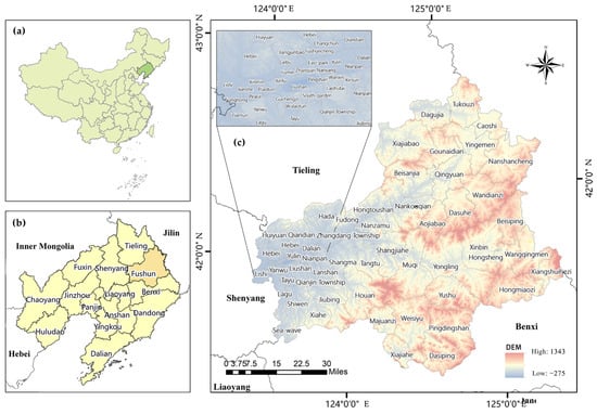
Figure 1.
Geographical location, digital elevation model (DEM), and overview of study area: (a) Liaoning Province’s position in country; (b) Fushun’s location in Liaoning Province; (c) administrative divisions of Fushun City at street scale.
As a vital green ecological barrier in Liaoning, Fushun plays a crucial role in water conservation and timber production in the province, with a forest coverage rate of 65.71%. The city experiences an average annual precipitation of 760–790 mm. Its topography is predominantly characterized by hills and mountains, with low rolling hills, undulating terrain, and narrow river valley plains in the central region. The urban area is situated on the Hunhe River alluvial plain, surrounded by mountains on three sides.
2.2. Research Framework
Based on the results of the investment model, this study constructs a progressive analytical framework (“single—factor analysis—interaction analysis—global regression—geographically weighted regression”) to study the driving mechanism of resource-exhausted cities. The proposed progressive analytical framework is illustrated in Figure 2.
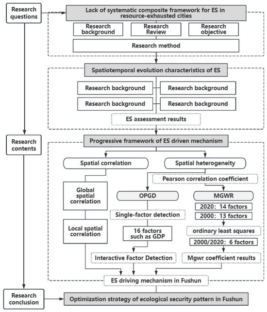
Figure 2.
Technology roadmap.
2.3. Data Sources and Description
The data used in this study encompass various aspects of Fushun City, including land use and land cover types, topography, natural climate conditions, socio-economic factors, and soil texture. The sources and detailed information are presented in Table 1. Slope data were derived from the DEM. All data were standardized to the GCS_Krasovsky_1940 projected coordinate system.

Table 1.
Data sources.
2.4. InVEST Model
2.4.1. Annual Water Yield Module
The annual water yield module in the InVEST model estimates the annual water yield within a region based on a water balance approach. This calculation incorporates factors such as annual precipitation, annual evapotranspiration, plant-available water content, and root depth. The formula is as follows:
Here, represents the annual water yield for each grid cell , denotes the actual annual evapotranspiration of grid cell , and refers to the annual precipitation at grid cell · represents the evapotranspiration component in the water balance, derived from the Budyko curve.
The evapotranspiration component of the water balance is derived from the Budyko curve formulation proposed by Fuh (1981) [46] and Zhang (2004) [47]. The parameter represents a non-physical variable characterizing the natural climate–soil properties. In this study, the expression proposed by Donohue et al. (2012) [48] is adopted. is a dimensionless dryness index [49], where denotes the crop coefficient, representing the ratio of actual to potential evapotranspiration. is the potential evapotranspiration (mm/day), which is calculated using a modified Hargreaves method [50]. is the Zhang coefficient, an empirical constant also referred to as the “seasonality factor” [51].
is the plant-available water content in volume (mm), estimated using nonlinear fitting methods [52]. Here , , , and represent the sand, silt, clay, and organic carbon contents in the soil, respectively.
2.4.2. SDR Module
The SDR module in the InVEST model calculates the annual soil erosion and retention using factors such as soil properties and rainfall. The soil retention value is determined by the difference between soil erosion reduction and soil loss. The model first calculates the soil erosion sediment yield for each grid cell, followed by the computation of the sediment delivery ratio (SDR), which represents the proportion of the total upstream soil erosion sediment that reaches the watershed outlet [53]. The annual soil erosion for each grid cell is estimated using the Revised Universal Soil Loss Equation (RUSLE) [54], expressed as follows:
In these equations, represents soil retention, is the potential soil erosion, and is the potential soil loss. is the rainfall erosivity factor, is the soil erodibility factor [55], represents the slope length and steepness factor, is the vegetation cover and crop management factor, and is the factor for soil conservation practices.
2.4.3. Carbon Storage
The carbon storage and sequestration module in the InVEST model estimates the total carbon stock based on user-provided land use maps and [56] carbon pool data. For Fushun City, the relevant carbon density data were compiled using existing research from Liaoning Province and other literature sources. The calculation is expressed as follows:
Here, , , , and represent the carbon stocks in the aboveground biomass, belowground biomass, dead organic matter, and soil, respectively.
2.4.4. Habitat Quality Module
The habitat quality module in the InVEST model assesses habitat quality by identifying ecosystem threat factors and their sensitivity. Based on previous studies, threat factors and their sensitivities to various land use types were defined. The formula is as follows:
In this formula, the impact of threat factor r in grid cell x on the habitat quality (HQ) of grid cell y is denoted as . The habitat quality of grid cell x in land use/land cover (LULC) type j is represented by Q. represents the habitat suitability of land type j, k is the half-saturation constant, and z is a scaling parameter reflecting spatial heterogeneity. denotes the total threat level for land type j in grid cell x. is the linear distance between grid cells x and y, and is the maximum effective distance over which threat factors r can exert influence.
2.5. Spatial Autocorrelation Analysis of Ecosystem Services
Spatial autocorrelation models are used to analyze the spatial clustering characteristics of various phenomena, specifically whether there are spatial dependencies or interactions between neighboring observations. In this study, we employed the global Moran’s I index and the local Moran’s I index to characterize the global and local clustering patterns of ecosystem services. The global Moran’s I index is defined as follows:
In this formula, N is the number of samples or spatial units, and represent the attribute values of spatial units i and j, respectively. is the mean attribute value of all spatial units. is the spatial weight between units i and j, which is typically defined based on spatial distance or adjacency. If i and j are adjacent, is nonzero (e.g., 1 or a distance-based weight); otherwise, ).
The local Moran’s I index is calculated as follows:
In this formula, is the local Moran’s I for spatial unit i. is the global variance of the attribute values.
2.6. Optimal Parameter-Based Geo-Detector (OPGD)
The Geo-detector model is a spatial statistical method used to quantify the influence of explanatory variables on a dependent variable and detect their interactions by analyzing the spatial heterogeneity of the data. Optimal Parameter-based Geo-detector (OPGD) is an advanced spatial analysis method that enhances traditional Geo-detector by optimizing parameter selection, improving the detection of driving factors and their interactions in complex geographical processes. In this study, we applied the single-factor detection and interaction-factor analysis of OPGD using R language’s geospatial data processing libraries and statistical tools. The Geo-detector assesses whether factor X significantly influences a target variable Y by calculating the explanatory power (q-value) of X on Y. The q-value is calculated as follows:
In this formula, h represents the category or partition and L is the total number of categories or partitions. is the sample size of category ℎ. is the variance of the target variable Y within category ℎ. N and are the total sample size and the overall variance of the target variable, respectively. Based on the optimal discretization tool provided in the “GD” package in R language, we selected the discretization method and the number of layers corresponding to the maximum q-value, determining the optimal parameter combination for factor analysis and interaction effect analysis. Informed by field investigations and previous studies, we comprehensively selected 16 driving factors from three dimensions: natural environment, economic development, and landscape patterns. These factors include: GDP, average elevation (EL), average slope (SLO), Proportion of Cultivated Land (Pcul), Proportion of Forest Land (PF), Proportion of Grassland (PG), Proportion of Water Area (PW), Proportion of Construction Land (Pcon), average temperature (AT), average precipitation (PRE), average NDVI, average NPP, land use intensity (LUI), road network density (RD), population density (PD), and nighttime light index (NTL).
2.7. OLS and MGWR Models
Ordinary Least Squares (OLS) is a classical statistical modeling approach used to estimate the parameters of a linear regression model. Its core principle involves minimizing the sum of squared residuals between the observed and predicted values to determine the best-fitting regression line. OLS analysis provides insights into whether the relationships between variables are significant and assesses the overall explanatory power of the model. Additionally, the Variance Inflation Factor (VIF) is calculated to check for severe multicollinearity among independent variables, helping to reduce errors in the MGWR model. The general OLS equation is as follows:
In this formula, is intercept of the model, is the regression coefficient of the k-th independent variable, and and are the values of the k-th independent variable for the i-th observation. ϵ represents the random error term, y is the dependent variable, K denotes the total number of independent variables, and is the regression coefficient of the k-th independent variable.
The geographically weighted regression (GWR) model is a spatial statistical technique that extends traditional regression by allowing coefficients to vary across locations, capturing spatial heterogeneity and revealing localized relationships between independent and dependent variables. Multi-scale geographically weighted regression (MGWR) is an extension of the geographically weighted regression (GWR) model, designed to analyze the multi-scale characteristics of spatial variations in the influence of explanatory variables on the dependent variable. MGWR improves the classic GWR model by allowing different explanatory variables to have varying spatial ranges of influence (bandwidths). Each explanatory variable is assigned a unique bandwidth, enabling the model to capture the varying scales of influence. The MGWR equation is as follows:
In this formula, is the dependent variable. is the intercept at the geographic location and is the spatially varying regression coefficient for the k-th explanatory variable, representing its influence on y at location . is the value of the k-th explanatory variable and is the residual term. W is the weight, and is the distance between points i and j. means the bandwidth or smoothing parameter. ϵ represents the random error term, y is the dependent variable, and K denotes the total number of independent variables.
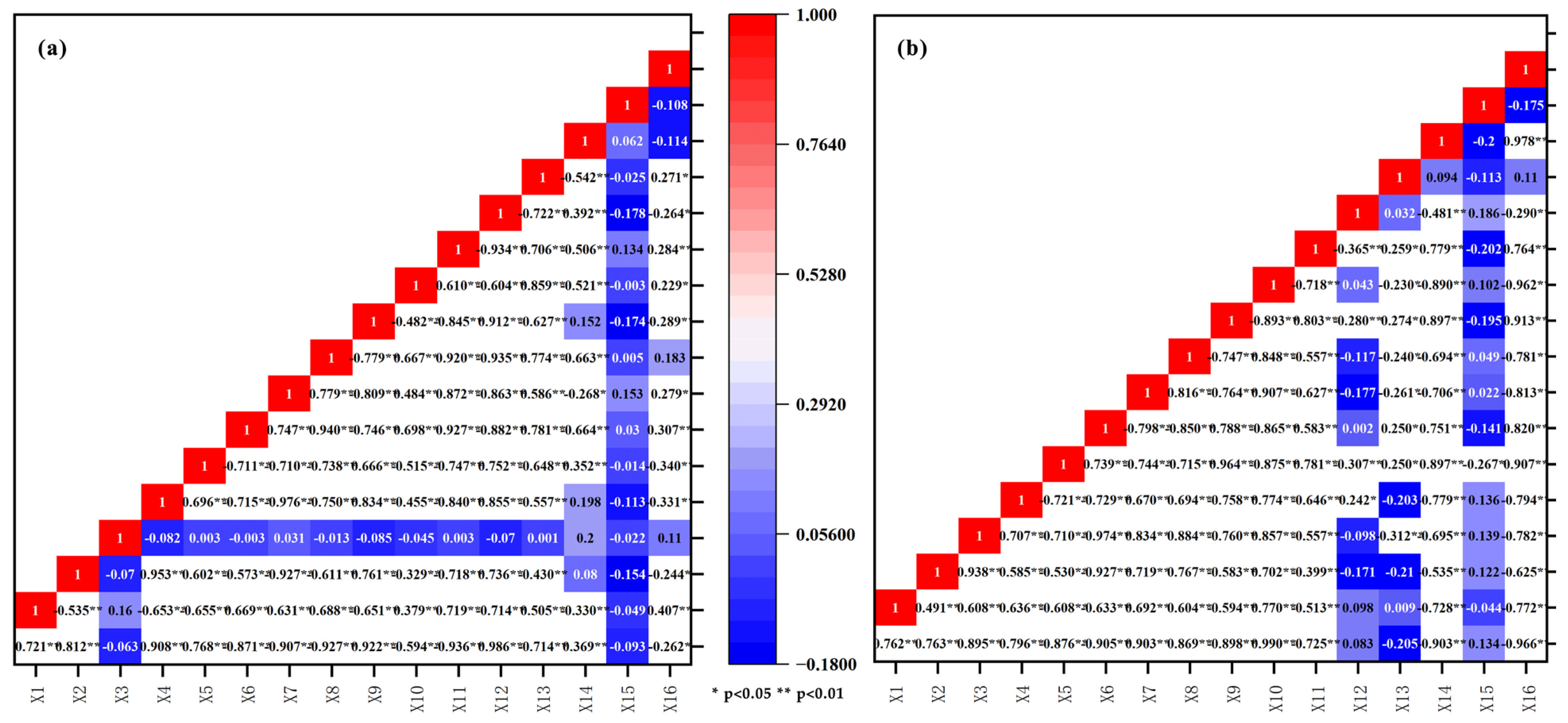
Before applying the multi-scale geographically weighted regression (MGWR) model, it is essential to conduct correlation analysis. Although the MGWR model inherently considers spatial heterogeneity and addresses spatial non-stationarity between dependent and independent variables, correlation analysis remains a critical step in model development. In this study, Pearson correlation analysis was performed using the corr function in R language, with 16 selected influencing factors. The results showed that, except for the proportions of water, grassland, and cultivated land, 13 potential influencing factors significantly impacted ecosystem services in 2000 (Figure A1).
3. Results
3.1. Spatiotemporal Evolution Characteristics of Ecosystem Services
Between 2000 and 2020, water supply volume and depth exhibited a consistent pattern of fluctuation with an overall increasing trend (Figure 3a), rising by 3.21 × 10⁹ m3 (an increase of 243.85%). The most significant growth occurred between 2000 and 2010 (76.92% increase), particularly in the first five years (~140%). This was followed by a decline of 1.53 × 10⁹ m3 (2010–2015) and a subsequent rebound of 1.27 × 10⁹ m3 (2015–2020), reaching the highest level in two decades. These changes were driven by government-led ecological restoration efforts, including a CNY 4.6 billion investment in wetland restoration (619 mu), tributary rehabilitation (13 rivers), and the establishment of the Dahuofang and Shehe Wetland Protected Areas, enhancing regional hydrological stability.
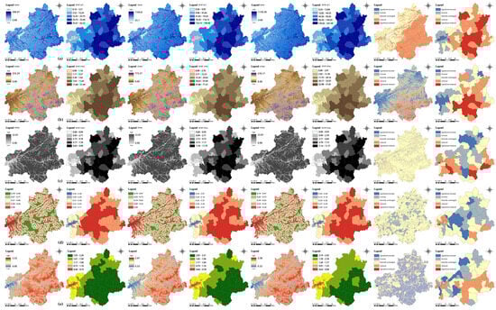
Figure 3.
The spatiotemporal evolution pattern of ecosystem services from 2000 to 2020: (a) WY: annual water yield; (b) SC: Sediment Delivery Yield; (c) CS: Carbon Storge; (d) HQ: habitat quality; (e) NES: Normalized ES.
Between 2000 and 2020, soil retention in Fushun City exhibited a fluctuating upward trend (Figure 3b), with a net increase of 0.48 × 10⁹ tons (133.33%). The most substantial growth (0.814 × 10⁹ tons, 76.92%) occurred from 2000 to 2010, particularly between 2005 and 2010 (~140%). However, from 2010 to 2015, soil retention declined sharply by 0.64 × 10⁹ tons (54.70%), primarily due to severe soil erosion caused by the catastrophic flood in 2013. In response, the Fushun government implemented large-scale soil and water conservation measures from 2015 to 2020, investing CNY 1.544 billion to restore 120.5 km2 of degraded land, effectively reducing sediment inflow into rivers and reservoirs. Concurrently, extensive mine geological restoration and land reclamation projects were carried out, with an investment of CNY 30.21 billion, rehabilitating 153.54 km2 of land. These efforts contributed to a subsequent rebound in soil retention (0.308 × 10⁹ tons, 58.49%), nearly reaching its peak value over the study period. Spatially, soil retention followed a “high in central areas, low in the west and southeast” pattern, with notable increases in the southern regions and significant decreases in the western and northeastern areas, reflecting the combined impact of natural disturbances and ecological restoration efforts.
Carbon storage showed an overall declining trend from 2000 to 2020 (Figure 3c), with a total reduction of 2.073 × 10⁶ tons (a decrease of approximately 0.92%). The most substantial changes occurred during 2005–2010 and 2015–2020, with reductions of 350,801 tons (0.15%) and 518,147 tons (0.23%), respectively. Although the reduction slowed between 2010 and 2020, carbon storage levels failed to recover to their 2000 values. Spatially, carbon storage exhibited a pattern of “low in the west and high in the southeast”, correlating with elevation.
The habitat quality index for Fushun City over five years was 0.985, 0.985, 0.970, 0.969, and 0.971, respectively, showing a general declining trend from 2000 to 2020 (Figure 3d). High-quality habitats were concentrated around Dahuofang Reservoir, while low-quality areas were mainly in the urban core. Severe degradation occurred in Hou’an Township, Tangtu Manchu Township, Weiziyu, Nanzaomu, Shangjiahe, and Caoshi Township, whereas Wanghua District saw improvements due to ecological restoration efforts. To restore its ecosystem, Fushun City established 906 km2 of ecological functional zones, reclaimed 31 km2 of farmland for afforestation, and restored 0.178 km2 of abandoned mines and 0.3753 km2 of active mining sites. However, in degraded areas, mining activities outpaced restoration efforts, limiting overall recovery.
Significant changes in ecosystem service capacity were observed in Fushun City from 2000 to 2020. Overall, ecosystem service capacity dynamics reflected a transition centered around medium-level service areas, accompanied by the expansion of low-capacity regions and degradation of high-capacity areas. This trend underscores the differentiation in ecosystem services during land use transformation. The expansion of low-capacity regions is associated with urbanization and ecological land development, whereas the degradation of high-capacity areas warrants greater attention. Protecting and restoring high-capacity regions while stabilizing medium-capacity zones are critical priorities for future ecological protection and management efforts.
3.2. Spatial Autocorrelation of Ecosystem Services
3.2.1. Global Spatial Autocorrelation
From 2000 to 2020, all ESs in Fushun City exhibited significant spatial autocorrelation, as evidenced by Moran’s I values that were statistically significant. Temporally, the Moran’s I values for water supply and soil retention showed an upward trend, indicating increasing spatial concentration of these services. In contrast, carbon storage exhibited minor spatial distribution changes, while habitat quality experienced a gradual decline, suggesting weakened spatial clustering. Among the global Moran’s I coefficients, habitat quality exhibited the highest values (0.796–0.828), followed by water supply and soil retention. Carbon storage had the lowest coefficients, ranging from 0.655 to 0.658 (Table A8).
3.2.2. Local Spatial Autocorrelation
Using global spatial autocorrelation as a baseline, local indicators of spatial association (LISA) maps were employed to identify clusters of strong local effects. Township-level mean values for various ecosystem services were calculated for univariate local spatial autocorrelation analysis, producing LISA maps for Fushun City from 2000 to 2020 (Figure 4).
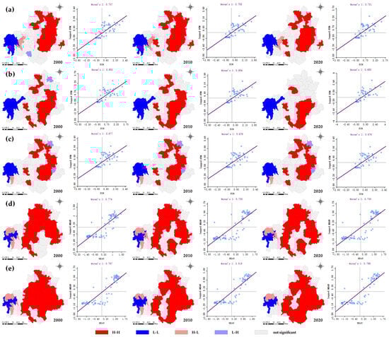
Figure 4.
Local autocorrelation map of ES space in Fushun City from 2000 to 2020: (a) WY: annual water yield; (b) SC: Sediment Delivery Yield; (c) CS: Carbon Storge; (d) HQ: habitat quality; (e) Es: Normalized Es.
The spatial distribution of water yield (WY) exhibited a high–high clustering pattern in the east and a low–low clustering pattern in the west. While low–low clusters remained stable from 2000 to 2020, high–high clusters peaked in 2010 before declining, with notable changes in Maquanzi Township, Tangtu Manchu Township, and Nanshancheng Town. Soil conservation (SC) showed high–high clustering in the southeast and northwest, while low–low clustering persisted in the west. A declining trend in high–high clusters post-2010 suggests a weakening of soil conservation functions. Carbon storage (CS) remained spatially stable, with high–high clusters in the east and low–low clusters in the west, indicating no major changes over time. Habitat quality (HQ) showed high–high clustering in the central and northeastern regions and low–low clustering in the southwest. The area of low–low clusters decreased, while high–high clusters fluctuated without a clear trend. Ecosystem services (ESs) followed a high–high clustering pattern in central and southern areas, whereas low–low clusters peaked in 2010 before declining. The overall trend indicates a fluctuating but diminishing concentration of high-value ecosystem services.
3.3. Single and Interactive Factors of OPGD
3.3.1. Factor Detection
Using the Optimal Partitioning Geographical Detector (OPGD) for factor detection, we identified five factors that passed the significance test in both 2000 and 2020 (Table 2).
Table 2.
2000, 2020 OPGD factor detector test results.
In 2000, GDP and average precipitation exhibited significant correlations with ESs, with high q-values reflecting their substantial driving effects. By 2020, the q-values of GDP, the land use composite index (LUI), and water area proportion increased significantly. The land use composite index replaced average precipitation as the second most influential factor, highlighting the growing importance of land use changes in shaping ESs.
Comparing the two periods, the q-value of GDP rose from 0.6897 in 2000 to 0.8545 in 2020, indicating that economic development increasingly drove ESs. Additionally, the significant rise in the q-value of the land use composite index (q = 0.3745, p < 0.001) in 2020 suggests that land use optimization or expansion played a more critical role in regulating ESs. This trend is likely linked to urban expansion and the optimization of land use structures.
3.3.2. Interactive Factor Detection
The q-values of interactive factor combinations reveal their explanatory power for the target phenomenon when acting together. If the combined q-value significantly exceeds that of individual factors, it indicates strong interaction effects.
In 2000 (Figure 5a), GDP and average precipitation exhibited a strong synergy (q = 0.9093), emerging as a key driver of ES changes. Similarly, GDP’s interactions with average elevation (q = 0.7647) and temperature (q = 0.8307) were substantial, indicating their collective influence. In contrast, forest area proportion showed limited interaction with other factors, suggesting a predominantly independent role. The interactions of cropland and built-up land proportions were generally weak, except when combined with water area proportion (q = 0.7743 and 0.7558, respectively), indicating moderate coupling effects under specific conditions. Overall, GDP, precipitation, and temperature were the dominant synergistic factors shaping ESs, with their combined q-value (0.9464) reinforcing their critical role.
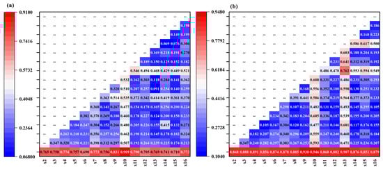
Figure 5.
OPGD interaction detector results: (a) 2000; (b) 2020.
By 2020 (Figure 5b), the synergy between GDP and precipitation intensified (q = 0.9464), alongside increased interactions between GDP and both elevation (q = 0.8681) and temperature (q = 0.9296), further highlighting their growing influence on ES dynamics. Additionally, the land use composite index and precipitation (q = 0.7622) exhibited strong coupling effects, emphasizing the role of land use patterns in shaping ES spatial distributions. Water area proportion’s interactions with GDP (q = 0.8782) and precipitation (q = 0.5862) underscored the increasing significance of water-related factors.
Compared to 2000, most interaction q-values increased in 2020, particularly for GDP (from 0.83 to 0.93) and water area proportion (from 0.77 to 0.88), reflecting the rising complexity of ES-driving mechanisms. This trend suggests that socio-economic development and land use transformation have intensified factor interactions, reinforcing their collective impact on ES evolution.
3.4. Analysis of Driving Mechanisms Using OLS and MGWR
3.4.1. Pearson Correlation Coefficient Analysis
The positive impact strength of the factors on ecosystem services was ranked as follows: forest land proportion > average NDVI > average elevation > average precipitation > population density > average slope. The negative impact strength was as follows: land use intensity > built-up land proportion > nighttime light index > average temperature > average NPP > GDP > road network density.
For 2020, 14 factors significantly influenced ecosystem services, excluding the land use intensity index and grassland proportion. Positive influences were ranked as follows: forestland proportion > average elevation > average slope > average NDVI > average precipitation > water body proportion. Negative influences were ranked as follows: built-up land proportion > nighttime light index > average temperature > average NPP > GDP > population density > road density > cultivated land proportion.
3.4.2. Global Regression Model: OLS
Based on the Variance Inflation Factor (VIF) and Pearson correlation results, a combination of variables was selected to balance statistical significance and model stability, reducing multicollinearity while preserving as much information as possible. The correlation matrix revealed high correlations (>|0.7|) among many variables, prompting the exclusion of highly collinear variables to ensure model independence and interpretability.
According to the OLS results (Table A7), in 2000, significant positive influencing factors included GDP, average precipitation, average slope, population density, and land use intensity, while the nighttime light index had a significant negative effect. In 2020, the significant positive influencing factors were average elevation, average NDVI, population density, and water proportion, whereas built-up land and cultivated land proportions had significant negative effects. GDP and road network density showed non-significant or near-significant impacts. The two non-significant factors were removed in the subsequent MGWR analysis.
3.4.3. Multi-Scale Geographically Weighted Regression Model: MGWR Model
- 1.
- Comparison Between Models
The comparison results demonstrate that the MGWR model exhibits superior performance over the global regression model (OLS), particularly in terms of log-likelihood and AICc values. The MGWR model is better equipped to handle spatial heterogeneity by capturing localized variations, making it more suitable for this case study. A comparison of diagnostic indicators between the OLS and MGWR models is presented in Table 3, demonstrating the superior explanatory power of the MGWR model.
Table 3.
Comparison between OLS model and MGWR model.
- 2.
- Results of MGWR Model
In 2000, GDP was positively correlated with ecosystem services (ESs), exhibiting a spatial pattern of “higher in the east, lower in the west” (Figure 6b). In rural areas, GDP growth promoted ES through natural resource-dependent activities like agriculture and forestry, enhancing carbon storage, water retention, and soil conservation. However, in urban areas, where GDP was mainly derived from industry and services, its impact on ES was indirect, as intensive human activity reduced its marginal benefits. Precipitation played a critical role in vegetation growth, enhancing carbon sequestration and water retention through photosynthesis and biomass accumulation. It exhibited a “lower in the east, higher in the west” pattern (Figure 6a). In the northwestern mountainous regions, increased precipitation notably improved ES, while in the central and southern basins, its effect diminished due to water saturation. Slope had a positive impact on ES, with a spatial distribution of “higher in the north, lower in the south” (Figure 6c). Steeper slopes in the northern and central hilly regions relied more on vegetation for soil conservation, reducing runoff and stabilizing soil, while these areas also demonstrated superior water regulation compared to flatter regions.
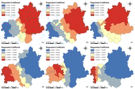
Figure 6.
Spatial distribution map of impact coefficients of various influencing factors in 2000: (a) PRE; (b) GDP; (c) SLO; (d) LUI; (e) PD; (f) NTL.
The Normalized Total Light (NTL), an indicator of urbanization, was negatively correlated with ES, showing a “higher in the west, lower in the east” pattern (Figure 6f). In rural areas, high NTL values often reflected agricultural expansion or low-density industrial development, leading to ecosystem degradation. In urban areas, however, the negative effects of NTL were mitigated by green spaces and technological systems, such as water recycling. Land use intensity had a significant negative relationship with ES, following a “higher in the west, lower in the east” distribution (Figure 6d). Increased land use intensity, especially the conversion of forests and grasslands to built-up areas or cropland, led to carbon storage decline and reduced soil retention, particularly in central hilly and western plain areas.
Between 2000 and 2020, the impact of population density on ES shifted from positive to negative (Figure 6e and Figure 7c), with spatial patterns transitioning from “northwest high, southeast low” in 2000 to “west high, southeast low” in 2020. Initially, higher population densities in the west were associated with ecological improvements through afforestation and infrastructure development. However, by 2020, increased population density in rural areas led to intensified agricultural activities, adversely affecting water provision, soil retention, and other ESs. In urban areas, natural vegetation was replaced by impervious surfaces, further diminishing ESs. Policies and technological interventions, such as green space expansion, partially mitigated these effects.
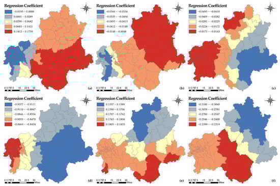
Figure 7.
Spatial distribution map of impact coefficients of various influencing factors in 2020: (a) NDVI; (b) PW; (c) PD; (d) Pcon; (e) EL; (f) Pcul.
Elevation indirectly influenced ESs by regulating climate, biological communities, and human activity distribution, following a “south high, north low” pattern (Figure 7e). High-altitude regions in the north, acting as ecological source areas, showed strong carbon storage capacity, contributing to carbon sequestration and water provision through precipitation and groundwater recharge. Improved vegetation, especially in the precipitation-rich southern regions, boosted carbon storage and enhanced soil permeability, promoting water resource replenishment (Figure 7a). However, its effects were weaker in the west, where urban expansion and resource exploitation constrained vegetation growth.
The expansion of built-up land led to reduced vegetation, increased impervious surfaces, diminished carbon storage, and weakened hydrological functions, heightening flood risks, significantly suppressing ESs, particularly in urban–rural transition zones. Areas with high cropland proportions saw reductions in carbon storage, soil degradation, and weakened water retention functions, exacerbated by long-term cultivation and intensive agricultural practices (Figure 7f). The expansion of water areas positively impacted water conservation, but in areas with steep slopes, it increased soil erosion risks. In urbanized areas, water bodies were negatively impacted by pollution and anthropogenic changes, reducing their ES provision (Figure 7b).
These results align with existing studies on the complex interactions among human activities, land use, and ecological processes. To enhance ESs, future strategies should focus on optimizing land use, improving vegetation cover, and balancing urban and agricultural development to promote sustainable ecological outcomes.
- 3.
- Changes in Driving Mechanisms (2000–2020)
In 2000, during the early stages of rapid urban development, ecosystem services were largely influenced by socio-economic factors such as GDP, population density, and NTL. Human activities, particularly agriculture and infrastructure development, had a direct positive impact on ecosystem services, including carbon storage, water retention, and soil conservation.
Starting in 2015, the focus shifted towards ecosystem restoration and land spatial planning, driven by policies aimed at ecological rehabilitation and territorial ecological management. These efforts, including reforestation and ecological restoration projects, began to significantly affect ecosystem services by enhancing natural factors like vegetation coverage and elevating the role of land use management. The implementation of these policies began to mitigate the degradation caused by urban expansion and agricultural intensification.
By 2020, natural factors such as NDVI and elevation, alongside changes in land use (e.g., urban expansion, agricultural intensification), became increasingly significant in driving ecosystem services. The shift from a purely socio-economic-driven model to one that integrates ecological restoration and sustainable land use reflects the growing complexity of interactions between human and natural systems.
Overall, from 2000 to 2020, the evolution of ecosystem service drivers moved from a focus on economic growth to a more integrated model, where ecological restoration and land use optimization play a critical role in sustaining ecosystem services.
4. Discussion
4.1. Comparison with Existing Studies
This study investigates the driving mechanisms of ecosystem services (ESs) in a resource-exhausted city from 2000 to 2020. By employing a progressive analytical framework of “single-factor analysis–interaction factor analysis–global regression analysis–multi-scale geographically weighted regression (MGWR) analysis”, this approach provides a comprehensive examination that integrates local and global perspectives, moving from single factors to interaction effects. The method effectively captures the spatial heterogeneity of ES drivers at different scales, particularly the influence of economic and land use factors in urban–rural transitional zones, thereby addressing the limitations of conventional single-factor analyses.
Existing studies have explored ES drivers across different regions and time periods. For instance, research on coalfield ecosystems in Shanxi Province identified temperature, precipitation, elevation (DEM), population size, urban land area, mining intensity, industrial output, and land use intensity as key influencing factors, with natural drivers playing a dominant role. The interaction between natural and human factors exhibited a stronger impact on ESs than individual factors alone [57]. While such findings highlight the interplay between socio-economic and environmental factors, they often fail to quantify the relative influence of different driving factors and capture their spatial heterogeneity.
This study addresses these gaps by refining the analytical scale to the street level in urban centers, compared to the conventional township-level analysis for entire cities. This finer spatial resolution enables a more precise assessment of ecosystem service dynamics in resource-exhausted cities. Additionally, the study proposes a progressive analytical framework, which not only provides robust conclusions for ecosystem management but also serves as a methodological reference for other resource-exhausted cities. By leveraging open-source data and models, the approach enhances reproducibility, while the selection of driving factors ensures both regional specificity and broader applicability. These contributions fill theoretical gaps and provide critical insights for sustainable urban transformation strategies.
4.2. Recommendations
4.2.1. Optimizing Land Use Structure to Enhance Ecosystem Services
The study indicates that the expansion of built-up areas and the high proportion of arable land are major negative factors affecting ecosystem services (ESs). In the early stages of rapid urban development (2000), built-up areas and intensive agricultural land use contributed to the degradation of ESs. By 2015, with the introduction of policies focused on ecological restoration and territorial land use optimization, a shift towards more sustainable land use practices began. Moving forward, urban expansion should be restricted through more stringent land use planning and policy controls, especially in critical ecological zones [58]. Ecological restoration projects—such as green corridors [59], urban wetlands, and vegetation buffers—should be prioritized to mitigate the adverse effects of urban sprawl. In rural areas, policies promoting eco-agricultural practices, including reduced cultivation intensity and sustainable irrigation techniques, will be essential to restore soil and water resources, while also enhancing farmland’s ecological functions.
4.2.2. Strengthening Ecosystem Management in Urban–Rural Transitional Zones
Land use changes in transitional zones significantly affect ESs [60]. In these areas, green infrastructure, optimized drainage systems, and increased vegetation cover should be prioritized to reduce ecological degradation. For less developed transitional zones, low-cost restoration measures such as vegetation recovery and wetland construction can be employed to restore ESs effectively.
4.2.3. Preserving Natural Factors and Utilizing Ecological Baseline Conditions
The positive roles of natural factors, such as elevation and NDVI, highlight the importance of preserving and optimizing natural conditions as the foundation for ecological restoration. From 2000 to 2020, the increasing significance of natural factors in driving ESs underscores the need to prioritize conservation in high-altitude ecological source areas and regions with intact vegetation, especially in the Gangshan and Tiannu Mountain areas [61]. Climate-adaptive management measures should be incorporated to ensure that these areas remain resilient to changing climatic conditions, further enhancing the stability and functionality of ecosystems.
4.2.4. Promoting Technological and Policy Synergies for Sustainable Development
To support long-term urban sustainability, integrating ecological technologies and policy tools is critical. The study emphasizes the shift towards more complex natural–social interactions in driving ESs by 2020, which calls for enhanced monitoring and management strategies. Ecological service compensation mechanisms should be introduced to attract private investment into ecological protection and restoration projects. Additionally, smart ecological monitoring technologies (e.g., remote sensing, big data analysis, and predictive models) should be utilized to track real-time changes in ESs. Policy efforts, such as those seen post-2015, should ensure these technologies and initiatives are effectively integrated into national and regional environmental strategies.
4.2.5. Addressing Climate Change by Building Resilient Ecosystems
Climate change is altering the patterns and drivers of ESs, a shift observed in the study between 2000 and 2020. In response, efforts to enhance regional climate adaptation capacity should include comprehensive ecological restoration initiatives, such as watershed restoration and sponge city construction, aimed at improving water retention and carbon storage capabilities [62,63]. Climate-adaptive policies, like those rolled out in 2015, must continue to evolve to mitigate the impacts of extreme weather on resource-depleted urban ecosystems, ensuring the continued stability of ES provision.
4.3. Limitations
This study analyzes changes in ecosystem services and their driving mechanisms in the resource-exhausted city of Fushun from 2000 to 2020. While the findings provide valuable insights, several limitations exist.
First, although the study covers two decades, the relatively recent end year may not fully capture the impacts of rapid urbanization and evolving ecological policies on ecosystem services. For example, the recent implementation of the “dual carbon” strategy [64,65] and advancements in technology, such as smart cities [66] and green infrastructure, may have caused significant fluctuations in ecological spaces and their services. These dynamic changes, however, were not included in the analysis. Future research should incorporate updated remote sensing data and socio-economic statistics, utilizing spatiotemporal dynamic models, such as GIS-based predictive simulations, to better capture evolving ecosystem service trends.
Second, while the study utilized a combined framework of single-factor and interaction-factor analysis, along with MGWR and geographic detectors, several critical factors were not addressed. Specifically, policy interventions [67,68], sociocultural influences [69], and institutional constraints, which could significantly affect land use patterns and ecological restoration, were not explicitly considered. Future research should adopt a more integrated framework that considers the complexities of socio-economic and natural systems, especially the role of policy in shaping ecosystem services [70].
Additionally, the complexity of factor interactions may exceed the explanatory power of the current models. While this study focused on the synergistic effects of key natural and human factors, it did not fully explore nonlinear relationships or feedback mechanisms among these factors, such as the impact of urban land expansion on carbon storage. Future work could leverage emerging techniques, like machine learning and system dynamics modeling, to uncover hidden relationships, particularly nonlinear and spatiotemporal interactions [71].
Finally, this study primarily focused on spatial heterogeneity at the street scale, which, though important for regional analysis, does not capture micro-level interactions between human activities and ecosystem services at finer resolutions (e.g., community or land parcel scales). Future studies should integrate finer-scale geographic units into multi-scale analyses [72] and examine cross-level coupling relationships (national, provincial, municipal, and street levels) to provide more targeted recommendations for ecological policy design.
5. Conclusions
Based on a progressive analytical framework, which integrates single-factor analysis, interaction-factor analysis, global regression analysis, and geographically weighted regression analysis, the research identifies the key spatiotemporal characteristics and driving factors of ES changes. The main conclusions are as follows:
- (1)
- The ESs in Fushun underwent varying degrees of change from 2000 to 2020: water provision and soil conservation showed an overall increasing trend, while carbon storage and habitat quality exhibited slight declines. Land use changes, climate factors, and policy measures played critical roles in these dynamics.
- (2)
- Single-factor analysis using the optimal parameter-based geographical detector revealed that GDP and average precipitation were the primary influencing factors in 2000, indicating the combined impact of natural conditions and economic activities. By 2020, GDP’s explanatory power had increased significantly, and the land use comprehensive index emerged as a key factor, highlighting the growing influence of economic development and land use changes on ESs.
- (3)
- Interaction analysis revealed significant synergistic effects and enhancement trends among drivers between 2000 and 2020. In 2000, the interaction between GDP and average precipitation or temperature had the highest explanatory power for spatial heterogeneity in ESs. By 2020, the synergy between GDP and precipitation intensified, with the Proportion of Water Area showing significant interactive effects with other factors. These findings underscore the central role of land use patterns in shaping ES changes.
- (4)
- Spatial heterogeneity analysis using the MGWR model indicated substantial changes in ES distribution and drivers from 2000 to 2020. In 2000, socio-economic variables, such as GDP, population density, and nighttime light indices, were key determinants, reflecting the direct regulatory role of human activities during early economic development. By 2020, the influence of natural factors and land use characteristics had grown, reflecting the increasing support of natural background conditions due to policies like reforestation and ecological restoration. MGWR results further revealed regional variations in factor impacts, such as the pronounced negative effects of built-up and arable land in transitional zones and the strong positive roles of elevation and NDVI in ecological source areas.
This study proposes a progressive analytical framework to explore the driving mechanisms behind ES changes in resource-exhausted cities like Fushun. By systematically analyzing these changes, the research provides valuable theoretical support for enhancing the ecological adaptability of human settlements and offers practical guidance for achieving sustainability goals.
Author Contributions
Conceptualization, Y.P. and Y.G.; methodology, Y.P.; software, Y.P.; validation, Y.P., Y.G., and H.Q.; formal analysis, Y.P.; investigation, Y.P.; resources, Y.P. and Y.G.; data curation, Y.P.; writing—original draft preparation, Y.P.; writing—review and editing, Y.P. and Y.G.; visualization, Y.P.; supervision, Y.P.; project administration, Y.G.; funding acquisition, Y.G. All authors have read and agreed to the published version of the manuscript.
Funding
This research was funded by the National Natural Science Foundation of China, grant number 42301256.
Data Availability Statement
The original contributions presented in the study are included in the article. All data used in this study are publicly available from the sources cited. Further inquiries can be directed to the corresponding author.
Conflicts of Interest
The authors declare no conflicts of interest.
Abbreviations
The following abbreviations are used in this manuscript:
| ESs | Ecosystem services |
| LULC | Land use and land cover |
| GWR | Geographically weighted regression |
| MGWR | Multi-scale geographically weighted regression |
| WY | Annual water yield |
| SDR | Sediment Delivery Ratio |
| HQ | Habitat quality |
| CS | Carbon storage |
| OPGD | The Optimal Parameter-based Geo-detector |
| OLS | Ordinary Least Squares |
| VIF | Variance Inflation Factor |
| EL | Average Elevation |
| SLO | Average Slope |
| Pcul | Proportion of Cultivated Land |
| PF | Proportion of Forest Land |
| PG | Proportion of Grassland |
| PW | Proportion of Water Area |
| Pcon | Proportion of Construction Land |
| AT | Average temperature |
| PRE | Average precipitation |
| LUI | Land use intensity |
| RD | Road network density |
| PD | Population density |
| NTL | Nighttime light index |
Appendix A
Table A1.
Table of biophysical coefficients in Fushun City.
Table A1.
Table of biophysical coefficients in Fushun City.
| LULC | Maximum Root Depth | Kc | LULC_Veg |
|---|---|---|---|
| cultivated land | 350 | 0.65 | 1 |
| forest | 3000 | 1 | 1 |
| grass | 2000 | 0.65 | 1 |
| water | 1 | 1 | 0 |
| construction land | 1 | 0.3 | 0 |
| unused land | 1 | 0.5 | 0 |
Table A2.
Parameters of vegetation coverage and management.
Table A2.
Parameters of vegetation coverage and management.
| LULC | C | P |
|---|---|---|
| cultivated land | 0.2 | 0.3 |
| forest | 0.006 | 1 |
| grass | 0.05 | 1 |
| water | 0 | 0 |
| construction land | 0 | 0 |
| unused land | 1 | 1 |
Table A3.
Carbon density of various land use types in Fushun City.
Table A3.
Carbon density of various land use types in Fushun City.
| LULC | C_Above | C_Below | C_Soil | C_Dead |
|---|---|---|---|---|
| cultivated land | 4.75 | 0 | 33.51 | 0 |
| forest | 53.55 | 26.8 | 170.56 | 2.56 |
| grass | 24.38 | 19.59 | 52.29 | 22.74 |
| water | 2.45 | 0.62 | 80.11 | 0.1 |
| construction land | 0 | 0 | 0 | 0 |
| unused land | 0 | 0 | 0 | 0 |
Table A4.
Weight table of ecological threat factors in Fushun City.
Table A4.
Weight table of ecological threat factors in Fushun City.
| Threat | Max_Dist | Weight | Decay |
|---|---|---|---|
| cultivated land | 7 | 0.8 | linear |
| construction land | 10 | 1 | index |
| unused land | 3 | 0.8 | linear |
Table A5.
Ecological sensitivity of different land use types in Fushun City.
Table A5.
Ecological sensitivity of different land use types in Fushun City.
| LULC | Habitat | Cultivated Land | Construction Land | Unused Land |
|---|---|---|---|---|
| cultivated land | 0 | 0 | 0 | 0 |
| forest | 1 | 0.8 | 0.8 | 0.5 |
| grass | 0.7 | 0.4 | 0.7 | 0.7 |
| water | 1 | 0.9 | 0.8 | 0.7 |
| construction land | 0 | 0 | 0 | 0 |
| unused land | 0 | 0 | 0 | 0 |
Table A6.
OLS results in 2000.
Table A6.
OLS results in 2000.
| Variable | Intercept | GDP | PRE | SLO | PD | NLI | LUI |
|---|---|---|---|---|---|---|---|
| coefficient | 0.088 | 0.641 | 0.532 | 1.037 | 0.408 | −0.47 | 0.575 |
| SD | 0.032 | 0.085 | 0.142 | 0.147 | 0.171 | 0.168 | 0.165 |
| t-values | 2.78 | 7.58 | 3.743 | 7.068 | 2.388 | −2.796 | 3.583 |
| VIF | - | 3.723 | 4.063 | 6.832 | 5.561 | 9.213 | 8.924 |
Table A7.
OLS results in 2020.
Table A7.
OLS results in 2020.
| Variable | Intercept | GDP | EL | NDVI | Pcon | PD | RD | Pcul | PW |
|---|---|---|---|---|---|---|---|---|---|
| coefficient | 0.021 | −0.023 | 0.879 | 1.615 | −0.197 | 0.346 | −0.026 | −0.269 | 0.33 |
| SD | 0.02 | 0.06 | 0.093 | 0.091 | 0.08 | 0.131 | 0.145 | 0.097 | 0.078 |
| t-values | 1.055 | −0.384 | 9.441 | 17.65 | −2.473 | 2.642 | −0.178 | −2.771 | 4.218 |
| VIF | - | 3.53 | 6.225 | 10.312 | 6.237 | 4.352 | 6.31 | 3.447 | 1.496 |
Table A8.
Global Moran’s I in Fushun City from 2000 to 2020.
Table A8.
Global Moran’s I in Fushun City from 2000 to 2020.
| Index | 2000 | 2010 | 2020 | |||||||||
|---|---|---|---|---|---|---|---|---|---|---|---|---|
| WY | SC | CS | HQ | WY | SC | CS | HQ | WY | SC | CS | HQ | |
| Moran’s I | 0.675 | 0.667 | 0.658 | 0.828 | 0.682 | 0.671 | 0.655 | 0.806 | 0.679 | 0.674 | 0.655 | 0.796 |
| E Index | −0.012 | −0.012 | −0.012 | −0.012 | −0.012 | −0.012 | −0.012 | −0.012 | −0.012 | −0.012 | −0.012 | −0.012 |
| variance | 0.0041 | 0.0041 | 0.0041 | 0.0042 | 0.0041 | 0.0041 | 0.0041 | 0.0042 | 0.0041 | 0.0041 | 0.0041 | 0.0042 |
| z-score | 10.688 | 10.565 | 10.394 | 12.933 | 10.805 | 10.648 | 10.346 | 12.585 | 10.738 | 10.717 | 10.354 | 12.427 |
| p-value | 0.000 | 0.000 | 0.000 | 0.000 | 0.000 | 0.000 | 0.000 | 0.000 | 0.000 | 0.000 | 0.000 | 0.000 |

Figure A1.
Pearson correlation results: (a) 2000; (b) 2020.
Figure A1.
Pearson correlation results: (a) 2000; (b) 2020.
References
- Costanza, R.; d’Arge, R.; De Groot, R.; Farber, S.; Grasso, M.; Hannon, B.; Limburg, K.; Naeem, S.; O’neill, R.V.; Paruelo, J.; et al. The value of the world’s ecosystem services and natural capital. Nature 1997, 387, 253–260. [Google Scholar] [CrossRef]
- Almenar, J.B.; Elliot, T.; Rugani, B.; Philippe, B.; Gutierrez, T.N.; Sonnemann, G.; Geneletti, D. Nexus between nature-based solutions, ecosystem services and urban challenges. Land Use Policy 2021, 100, 104898. [Google Scholar] [CrossRef]
- Andersson, E.; Barthel, S.; Borgström, S.; Colding, J.; Elmqvist, T.; Folke, C.; Gren, Å. Reconnecting cities to the biosphere: Stewardship of green infrastructure and urban ecosystem services. Ambio 2014, 43, 445–453. [Google Scholar] [CrossRef] [PubMed]
- Boyanova, K.; Nedkov, S.; Burkhard, B. Applications of GIS-based hydrological models in mountain areas in Bulgaria for ecosystem services assessment: Issues and advantages. In Sustainable Mountain Regions: Challenges and Perspectives in Southeastern Europe; Springer: New York, NY, USA, 2016; pp. 35–51. [Google Scholar]
- Basse, R.M.; Omrani, H.; Charif, O.; Gerber, P.; Bódis, K. Land use changes modelling using advanced methods: Cellular automata and artificial neural networks. The spatial and explicit representation of land cover dynamics at the cross-border region scale. Appl. Geogr. 2014, 53, 160–171. [Google Scholar] [CrossRef]
- Rimal, B.; Sharma, R.; Kunwar, R.; Keshtkar, H.; Stork, N.E.; Rijal, S.; Rahman, S.A.; Baral, H. Effects of land use and land cover change on ecosystem services in the Koshi River Basin, Eastern Nepal. Ecosyst. Serv. 2019, 38, 100963. [Google Scholar] [CrossRef]
- Gomes, E.; Inácio, M.; Bogdzevič, K.; Kalinauskas, M.; Karnauskaitė, D.; Pereira, P. Future land-use changes and its impacts on terrestrial ecosystem services: A review. Sci. Total Environ. 2021, 781, 146716. [Google Scholar] [CrossRef]
- Zhang, Z.; Liu, Y.; Wang, Y.; Liu, Y.; Zhang, Y.; Zhang, Y. What factors affect the synergy and tradeoff between ecosystem services, and how, from a geospatial perspective? J. Clean. Prod. 2020, 257, 120454. [Google Scholar] [CrossRef]
- Tallis, H.; Ricketts, T.; Guerry, A.; Nelson, E.; Ennaanay, D.; Wolny, S.; Olwero, N.; Vigerstol, K.; Pennington, D.; Mendoza, G. InVEST 2.1 Beta User’s Guide. The Natural Capital Project. 2011. Available online: https://storage.googleapis.com/releases.naturalcapitalproject.org/invest-userguide/latest/en/index.html (accessed on 25 November 2024).
- Yu, Y.; Xiao, Z.; Bruzzone, L.; Deng, H. Mapping and Analyzing the Spatiotemporal Patterns and Drivers of Multiple Ecosystem Services: A Case Study in the Yangtze and Yellow River Basins. Remote Sens. 2024, 16, 411. [Google Scholar] [CrossRef]
- Yang, J.; Zhai, D.-L.; Fang, Z.; Alatalo, J.M.; Yao, Z.; Yang, W.; Su, Y.; Bai, Y.; Zhao, G.; Xu, J. Changes in and driving forces of ecosystem services in tropical southwestern China. Ecol. Indic. 2023, 149, 110180. [Google Scholar] [CrossRef]
- Zhou, Y.; Chen, T.; Wang, J.; Xu, X. Analyzing the Factors Driving the Changes of Ecosystem Service Value in the Liangzi Lake Basin—A GeoDetector-Based Application. Sustainability 2023, 15, 15763. [Google Scholar] [CrossRef]
- Deng, C.; Shen, X.; Liu, C.; Liu, Y. Spatiotemporal characteristics and socio-ecological drivers of ecosystem service interactions in the Dongting Lake Ecological Economic Zone. Ecol. Indic. 2024, 167, 112734. [Google Scholar] [CrossRef]
- Wang, C.; Ma, L.; Zhang, Y.; Chen, N.; Wang, W.J. Spatiotemporal dynamics of wetlands and their driving factors based on PLS-SEM: A case study in Wuhan. Sci. Total Environ. 2022, 806, 151310. [Google Scholar] [CrossRef] [PubMed]
- Lyu, R.; Clarke, K.C.; Zhang, J.; Feng, J.; Jia, X.; Li, J. Spatial correlations among ecosystem services and their socio-ecological driving factors: A case study in the city belt along the Yellow River in Ningxia, China. Appl. Geogr. 2019, 108, 64–73. [Google Scholar] [CrossRef]
- Han, P.; Hu, H.; Zhou, J.; Wang, M.; Zhou, Z. Integrating key ecosystem services to study the spatio-temporal dynamics and determinants of ecosystem health in Wuhan’s central urban area. Ecol. Indic. 2024, 166, 112352. [Google Scholar] [CrossRef]
- Kang, J.; Li, C.; Zhang, B.; Zhang, J.; Li, M.; Hu, Y. How do natural and human factors influence ecosystem services changing? A case study in two most developed regions of China. Ecol. Indic. 2023, 146, 109891. [Google Scholar] [CrossRef]
- Geng, T.W.; Chen, H.; Zhang, H.; Shi, Q.Q.; Liu, D. Spatiotemporal evolution of land ecosystem service value and its influencing factors in Shaanxi province based on GWR. J. Nat. Resour. 2020, 35, 1714–1727. [Google Scholar]
- Liu, W.; Zhan, J.; Zhao, F.; Wang, C.; Zhang, F.; Teng, Y.; Chu, X.; Kumi, M.A. Spatio-temporal variations of ecosystem services and their drivers in the Pearl River Delta, China. J. Clean. Prod. 2022, 337, 130466. [Google Scholar] [CrossRef]
- Xiao, Y.; Zhong, J.-L.; Zhang, Q.-F.; Xiang, X.; Huang, H. Exploring the coupling coordination and key factors between urbanization and land use efficiency in ecologically sensitive areas: A case study of the Loess Plateau, China. Sustain. Cities Soc. 2022, 86, 104148. [Google Scholar] [CrossRef]
- Xu, G.; Jiang, Y.; Wang, S.; Qin, K.; Ding, J.; Liu, Y.; Lu, B. Spatial disparities of self-reported COVID-19 cases and influencing factors in Wuhan, China. Sustain. Cities Soc. 2022, 76, 103485. [Google Scholar] [CrossRef]
- Wu, Y.; Wu, Y.; Li, C.; Gao, B.; Zheng, K.; Wang, M.; Deng, Y.; Fan, X. Spatial relationships and impact effects between urbanization and ecosystem health in urban agglomerations along the Belt and Road: A case study of the Guangdong-Hong Kong-Macao Greater Bay Area. Int. J. Environ. Res. Public Health 2022, 19, 16053. [Google Scholar] [CrossRef]
- Fotheringham, A.S.; Brunsdon, C.; Charlton, M. Geographically weighted regression. Sage Handb. Spat. Anal. 2009, 1, 243–254. [Google Scholar]
- Yu, P.; Zhang, S.; Yung, E.H.; Chan, E.H.; Luan, B.; Chen, Y. On the urban compactness to ecosystem services in a rapidly urbanising metropolitan area: Highlighting scale effects and spatial non-stationary. Environ. Impact Assess. Rev. 2023, 98, 106975. [Google Scholar] [CrossRef]
- Shilong, W.; Lufeng, Y.; Ting, Z.; Rongfang, L.; Yuliang, W.; Zilong, Z. The effects of landscape patterns on ecosystem services of urban agglomeration in semi-arid area under scenario modeling. Ecol. Indic. 2024, 167, 112610. [Google Scholar] [CrossRef]
- Yu, H.; Yang, J.; Sun, D.; Li, T.; Liu, Y. Spatial Responses of Ecosystem Service Value during the Development of Urban Agglomerations. Land 2022, 11, 165. [Google Scholar] [CrossRef]
- Li, S.; Xiao, W.; Zhao, Y.; Lv, X. Incorporating ecological risk index in the multi-process MCRE model to optimize the ecological security pattern in a semi-arid area with intensive coal mining: A case study in northern China. J. Clean. Prod. 2020, 247, 119143. [Google Scholar] [CrossRef]
- Jiang, S.; Feng, F.; Zhang, X.; Xu, C.; Jia, B.; Lafortezza, R. Ecological transformation is the key to improve ecosystem health for resource-exhausted cities: A case study in China based on future development scenarios. Sci. Total Environ. 2024, 921, 171147. [Google Scholar] [CrossRef]
- Yu, S.; Wang, R.; Zhang, X.; Miao, Y.; Wang, C. Spatiotemporal Evolution of Urban Shrinkage and Its Impact on Urban Resilience in Three Provinces of Northeast China. Land 2023, 12, 1412. [Google Scholar] [CrossRef]
- Clark, M.; Hall, K.R.; Martin, D.M.; Beaty, B.; Lloyd, S.; Galgamuwa, G.P.; Shirer, R.; Zimmerman, C.L.; Shallows, K.M. Prioritizing restoration sites that improve connectivity in the Appalachian landscape, USA. Conserv. Sci. Pract. 2023, 5, e13046. [Google Scholar] [CrossRef]
- Peng, J.; Xu, Y.; Cai, Y.; Xiao, H. The role of policies in land use/cover change since the 1970s in ecologically fragile karst areas of Southwest China: A case study on the Maotiaohe watershed. Environ. Sci. Policy 2011, 14, 408–418. [Google Scholar] [CrossRef]
- Ding, T.; Chen, J.; Fang, Z.; Chen, J. Assessment of coordinative relationship between comprehensive ecosystem service and urbanization: A case study of Yangtze River Delta urban Agglomerations, China. Ecol. Indic. 2021, 133, 108454. [Google Scholar] [CrossRef]
- Fang, Z.; Bai, Y.; Jiang, B.; Alatalo, J.M.; Liu, G.; Wang, H. Quantifying variations in ecosystem services in altitude-associated vegetation types in a tropical region of China. Sci. Total Environ. 2020, 726, 138565. [Google Scholar] [CrossRef] [PubMed]
- Wu, Y.; Tao, Y.; Yang, G.; Ou, W.; Pueppke, S.; Sun, X.; Chen, G.; Tao, Q. Impact of land use change on multiple ecosystem services in the rapidly urbanizing Kunshan City of China: Past trajectories and future projections. Land Use Policy 2019, 85, 419–427. [Google Scholar] [CrossRef]
- Ge, G.; Zhang, J.; Chen, X.; Liu, X.; Hao, Y.; Yang, X.; Kwon, S. Effects of land use and land cover change on ecosystem services in an arid desert-oasis ecotone along the Yellow River of China. Ecol. Eng. 2022, 176, 106512. [Google Scholar] [CrossRef]
- Su, K.; Liu, H.; Wang, H. Spatial–temporal changes and driving force analysis of ecosystems in the Loess Plateau Ecological Screen. Forests 2022, 13, 54. [Google Scholar] [CrossRef]
- Liu, Q.; Qiao, J.; Li, M.; Huang, M. Spatiotemporal heterogeneity of ecosystem service interactions and their drivers at different spatial scales in the Yellow River Basin. Sci. Total Environ. 2024, 908, 168486. [Google Scholar] [CrossRef]
- Fang, Z.; Ding, T.; Chen, J.; Xue, S.; Zhou, Q.; Wang, Y.; Wang, Y.; Huang, Z.; Yang, S. Impacts of land use/land cover changes on ecosystem services in ecologically fragile regions. Sci. Total Environ. 2022, 831, 154967. [Google Scholar] [CrossRef]
- Pan, N.; Guan, Q.; Wang, Q.; Sun, Y.; Li, H.; Ma, Y. Spatial Differentiation and Driving Mechanisms in Ecosystem Service Value of Arid Region: A case study in the middle and lower reaches of Shule River Basin, NW China. J. Clean. Prod. 2021, 319, 128718. [Google Scholar] [CrossRef]
- Liu, X.; Duan, Z.; Shan, Y.; Duan, H.; Wang, S.; Song, J.; Wang, X. Low-carbon developments in Northeast China: Evidence from cities. Appl. Energy 2019, 236, 1019–1033. [Google Scholar] [CrossRef]
- Guo, C.-J.; Liu, Y.-X.; Li, H.-F.; Sun, Y.-T.; Yu, Y.-C. Landscape characteristics and construction of landscape ecological security pattern in West Open Pit of Fushun mine. J. Shenyang Agric. Univ. 2021, 52, 442–450. [Google Scholar]
- Peng, J.; Li, S.; Xiaoji, H.; Ji, G.; Maomao, W. Control. Spatial-temporal distribution characteristics and influencing factors of geological disasters in the open-pit mining area of western Fushun, Liaoning Province. Chin. J. Geol. Hazard Control 2022, 33, 68–76. [Google Scholar]
- Xu, H.; Cheng, W. Landscape Analysis and Ecological Risk Assessment during 1995–2020 Based on Land Utilization/Land Coverage (LULC) and Random Forest: A Case Study of the Fushun Open-Pit Coal Area in Liaoning, China. Sustainability 2024, 16, 2442. [Google Scholar] [CrossRef]
- Xiao, P.; Yan, X.; Wang, X.; Deng, Y.; Xie, S.; Sun, L.; Xing, Y. Research on Ecological Protection and Restoration Technology of Fushun West Open pit Mine in Liaoning Province. Adv. Eng. Technol. Res. 2024, 12, 188. [Google Scholar] [CrossRef]
- Yan, F.; Shangguan, W.; Zhang, J.; Hu, B. Depth-to-bedrock map of China at a spatial resolution of 100 meters. Sci. Data 2020, 7, 2. [Google Scholar] [CrossRef]
- Fuh, B.-p. On the calculation of the evaporation from land surface. Chin. J. Atmos. Sci. 1981, 5, 23–31. [Google Scholar] [CrossRef]
- Zhang, L.; Hickel, K.; Dawes, W.R.; Chiew, F.H.S.; Western, A.W.; Briggs, P.R. A rational function approach for estimating mean annual evapotranspiration. Water Resour. Res. 2004, 40, 89–97. [Google Scholar] [CrossRef]
- Donohue, R.J.; Roderick, M.L.; McVicar, T.R. Roots, storms and soil pores: Incorporating key ecohydrological processes into Budyko’s hydrological model. J. Hydrol. 2012, 436, 35–50. [Google Scholar] [CrossRef]
- Budyko, M.I.; Miller, D.H. Climate and Life; Academic Press: London, UK, 1974. [Google Scholar]
- Berti, A.; Tardivo, G.; Chiaudani, A.; Rech, F.; Borin, M. Assessing reference evapotranspiration by the Hargreaves method in north-eastern Italy. Agric. Water Manag. 2014, 140, 20–25. [Google Scholar] [CrossRef]
- Lv, L.; Li, Q.; Yang, Y. Change and influencing factors of water conservation in Liaoning province during 2001—2020. Bull. Soil Water Conserv. 2022, 42, 290–296. [Google Scholar]
- Zhou, W.Z.; Liu, G.H.; Pan, J.J. Soil Available Water Capacity and it’s Empirical and Statistical Models-with Special Reference to Black Soils in Northeast China. J. Arid. Land Resour. Environ. 2003, 4, 88–95. [Google Scholar]
- Borselli, L.; Cassi, P.; Torri, D. Prolegomena to sediment and flow connectivity in the landscape: A GIS and field numerical assessment. Catena 2008, 75, 268–277. [Google Scholar] [CrossRef]
- Renard, K.G.; Freimund, J.R. Using monthly precipitation data to estimate the R-factor in the revised USLE. J. Hydrol. 1994, 157, 287–306. [Google Scholar] [CrossRef]
- Lychuk, T.E.; Izaurralde, R.C.; Hill, R.L.; McGill, W.B.; Williams, J.R. Biochar as a global change adaptation: Predicting biochar impacts on crop productivity and soil quality for a tropical soil with the Environmental Policy Integrated Climate (EPIC) model. Mitig. Adapt. Strat. Glob. Change 2015, 20, 1437–1458. [Google Scholar] [CrossRef]
- Li, P.; Chen, J.; Li, Y.; Wu, W. Using the InVEST-PLUS Model to Predict and Analyze the Pattern of Ecosystem Carbon storage in Liaoning Province, China. Remote Sens. 2023, 15, 4050. [Google Scholar] [CrossRef]
- Pan, H.; Wang, J.; Du, Z.; Wu, Z.; Zhang, H.; Ma, K. Spatiotemporal evolution of ecosystem services and its potential drivers in coalfields of Shanxi Province, China. Ecol. Indic. 2023, 148, 110109. [Google Scholar] [CrossRef]
- Bai, Y.; Wong, C.P.; Jiang, B.; Hughes, A.C.; Wang, M.; Wang, Q. Developing China’s Ecological Redline Policy using ecosystem services assessments for land use planning. Nat. Commun. 2018, 9, 3034. [Google Scholar] [CrossRef]
- Shi, X.; Zhou, F.; Wang, Z. Research on optimization of ecological service function and planning control of land resources planning based on ecological protection and restoration. Environ. Technol. Innov. 2021, 24, 101904. [Google Scholar] [CrossRef]
- Baró, F.; Gómez-Baggethun, E.; Haase, D. Ecosystem service bundles along the urban-rural gradient: Insights for landscape planning and management. Ecosyst. Serv. 2017, 24, 147–159. [Google Scholar] [CrossRef]
- Li, S.; Zhao, X.; Pu, J.; Miao, P.; Wang, Q.; Tan, K. Optimize and control territorial spatial functional areas to improve the ecological stability and total environment in karst areas of Southwest China. Land Use Policy 2021, 100, 104940. [Google Scholar] [CrossRef]
- McPhearson, T.; Andersson, E.; Elmqvist, T.; Frantzeskaki, N. Resilience of and through urban ecosystem services. Ecosyst. Serv. 2015, 12, 152–156. [Google Scholar] [CrossRef]
- McPhearson, T.; Hamstead, Z.A.; Kremer, P. Urban ecosystem services for resilience planning and management in New York City. Ambio 2014, 43, 502–515. [Google Scholar] [CrossRef]
- Liu, J.; Yan, Q.; Zhang, M.J.S.o.T.T.E. Ecosystem carbon storage considering combined environmental and land-use changes in the future and pathways to carbon neutrality in developed regions. Ecosyst. Serv. 2023, 903, 166204. [Google Scholar] [CrossRef] [PubMed]
- Liu, M.; Dong, X.; Wang, X.-C.; Zhao, B.; Fan, W.; Wei, H.; Zhang, P.; Liu, R. Evaluating the future terrestrial ecosystem contributions to carbon neutrality in Qinghai-Tibet Plateau. J. Clean. Prod. 2022, 374, 133914. [Google Scholar] [CrossRef]
- Siedlarczyk, E.; Winczek, M.; Zięba-Kulawik, K.; Wężyk, P. Smart green infrastructure in a smart city–the case study of ecosystem services evaluation in krakow based on i-Tree eco software. Geosci. Eng. 2019, 65, 36–43. [Google Scholar] [CrossRef]
- Corbera, E.; Soberanis, C.G.; Brown, K. Institutional dimensions of Payments for Ecosystem Services: An analysis of Mexico’s carbon forestry programme. Ecol. Econ. 2009, 68, 743–761. [Google Scholar] [CrossRef]
- Guo, X.; Zhang, Y.; Guo, D.; Lu, W.; Xu, H. How does ecological protection redline policy affect regional land use and ecosystem services? Environ. Impact Assess. Rev. 2023, 100, 107062. [Google Scholar] [CrossRef]
- Iniesta-Arandia, I.; García-Llorente, M.; Aguilera, P.A.; Montes, C.; Martín-López, B. Socio-cultural valuation of ecosystem services: Uncovering the links between values, drivers of change, and human well-being. Ecol. Econ. 2014, 108, 36–48. [Google Scholar] [CrossRef]
- Lü, Y.; Fu, B.; Feng, X.; Zeng, Y.; Liu, Y.; Chang, R.; Sun, G.; Wu, B. A policy-driven large scale ecological restoration: Quantifying ecosystem services changes in the loess plateau of China. PLoS ONE 2012, 7, e31782. [Google Scholar] [CrossRef]
- Ren, Q.; Liu, D.; Liu, Y.; Liu, Y. Spatio-temporal dynamics and socio-ecological determinants of ecosystem service interplays in Shandong Province’s coastal region (2000–2020): Implications for environmental protection and sustainable ecosystem management. Environ. Res. 2024, 243, 117824. [Google Scholar] [CrossRef]
- Chen, Y.; Lu, Y.; Meng, R.; Li, S.; Zheng, L.; Song, M. Multi-scale matching and simulating flows of ecosystem service supply and demand in the Wuhan metropolitan area, China. J. Clean. Prod. 2024, 476, 143648. [Google Scholar] [CrossRef]
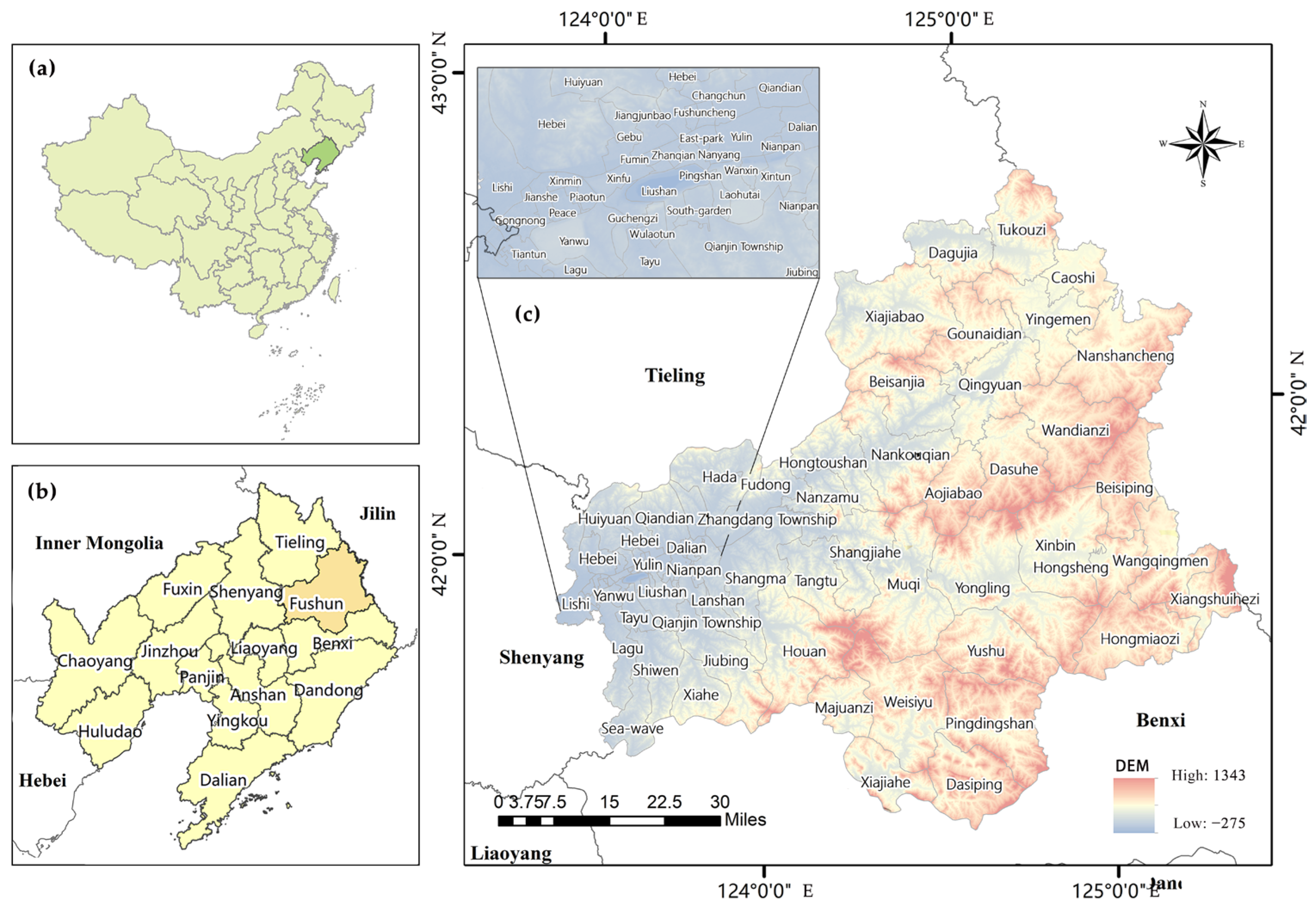
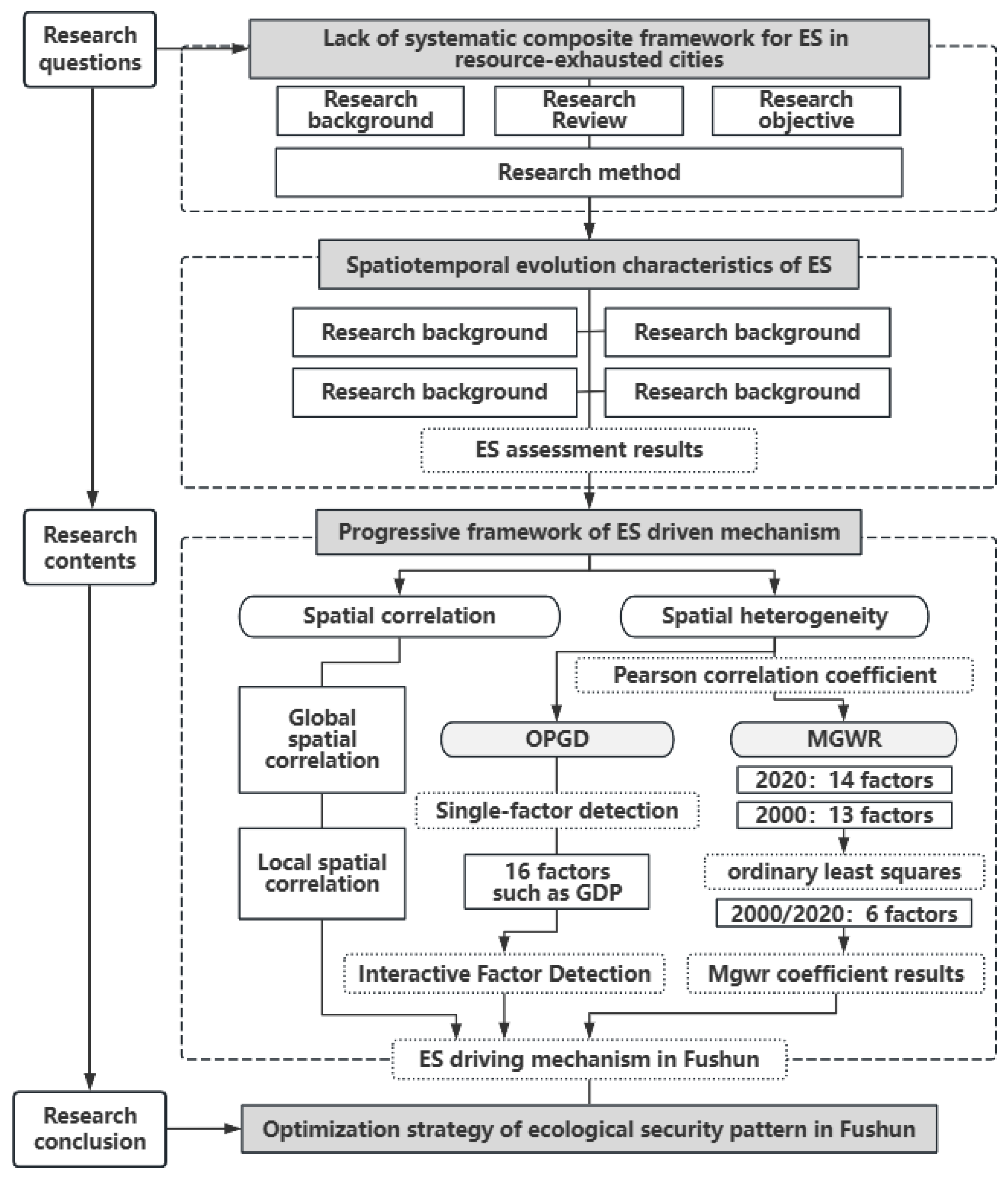
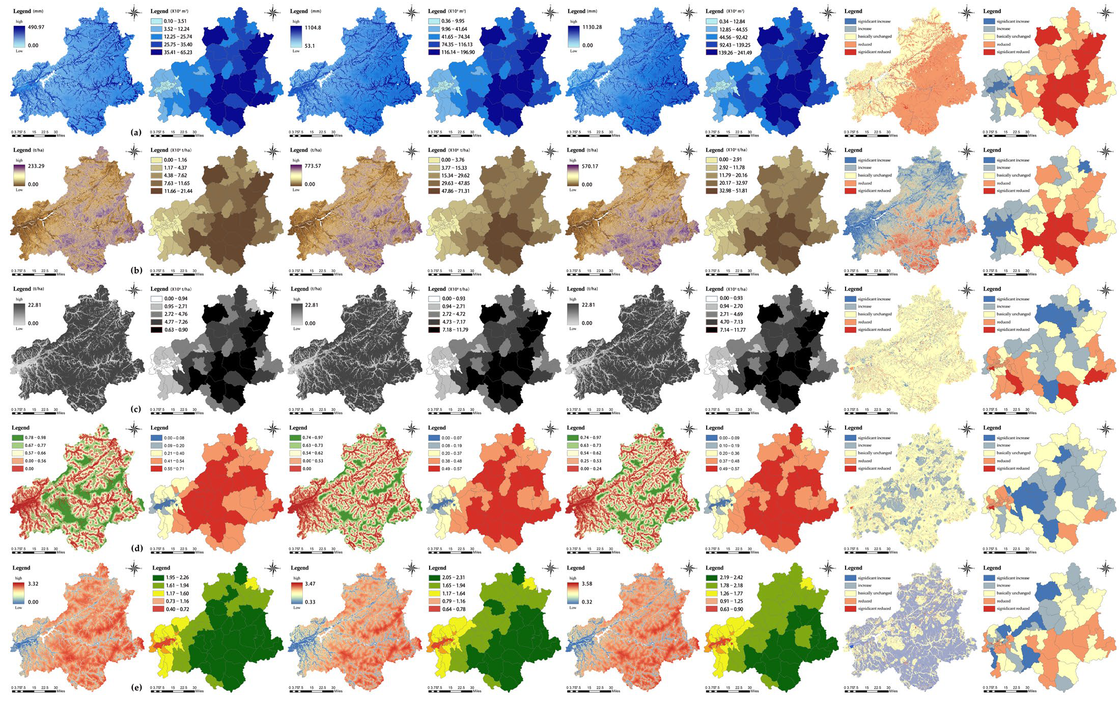
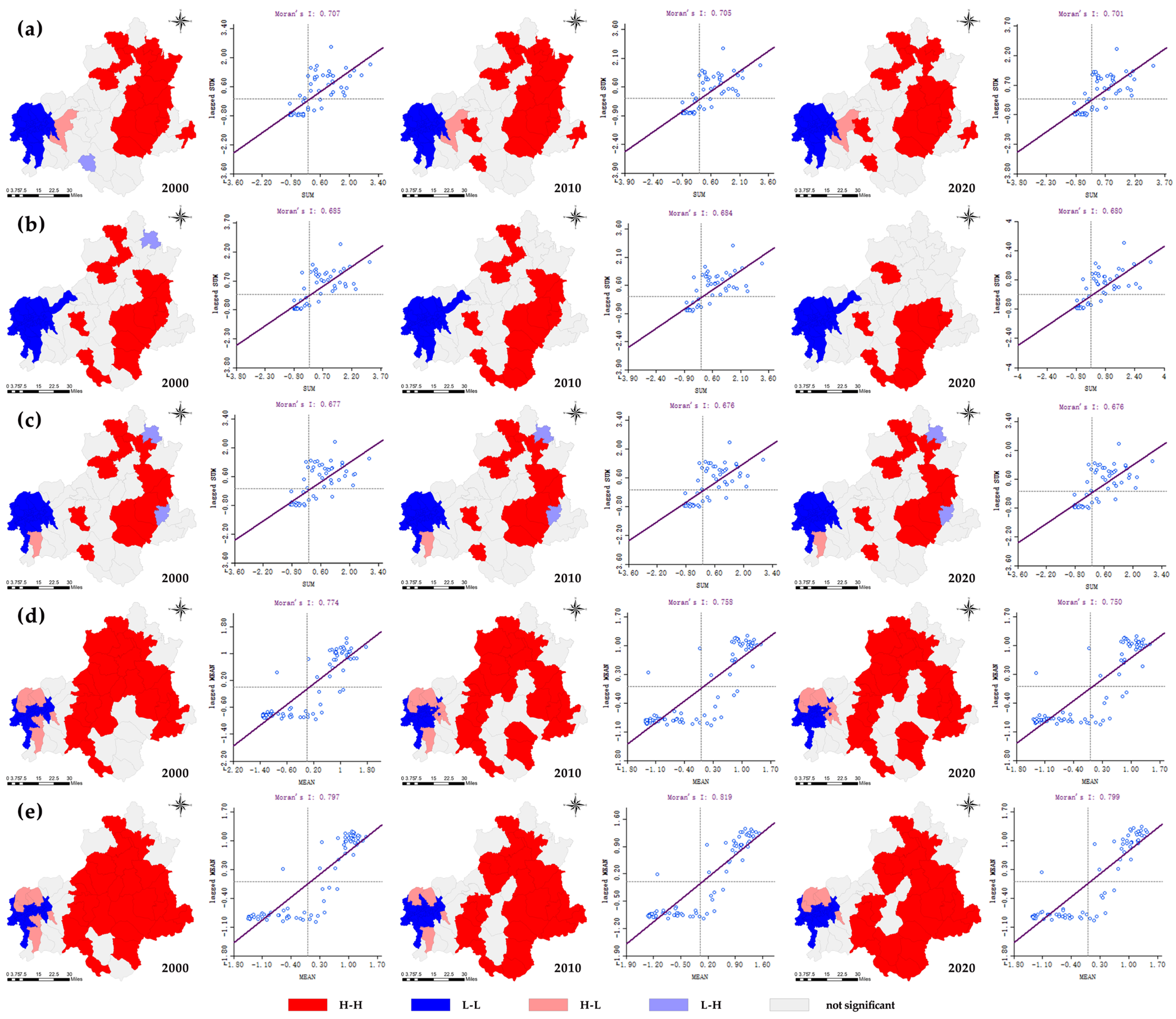

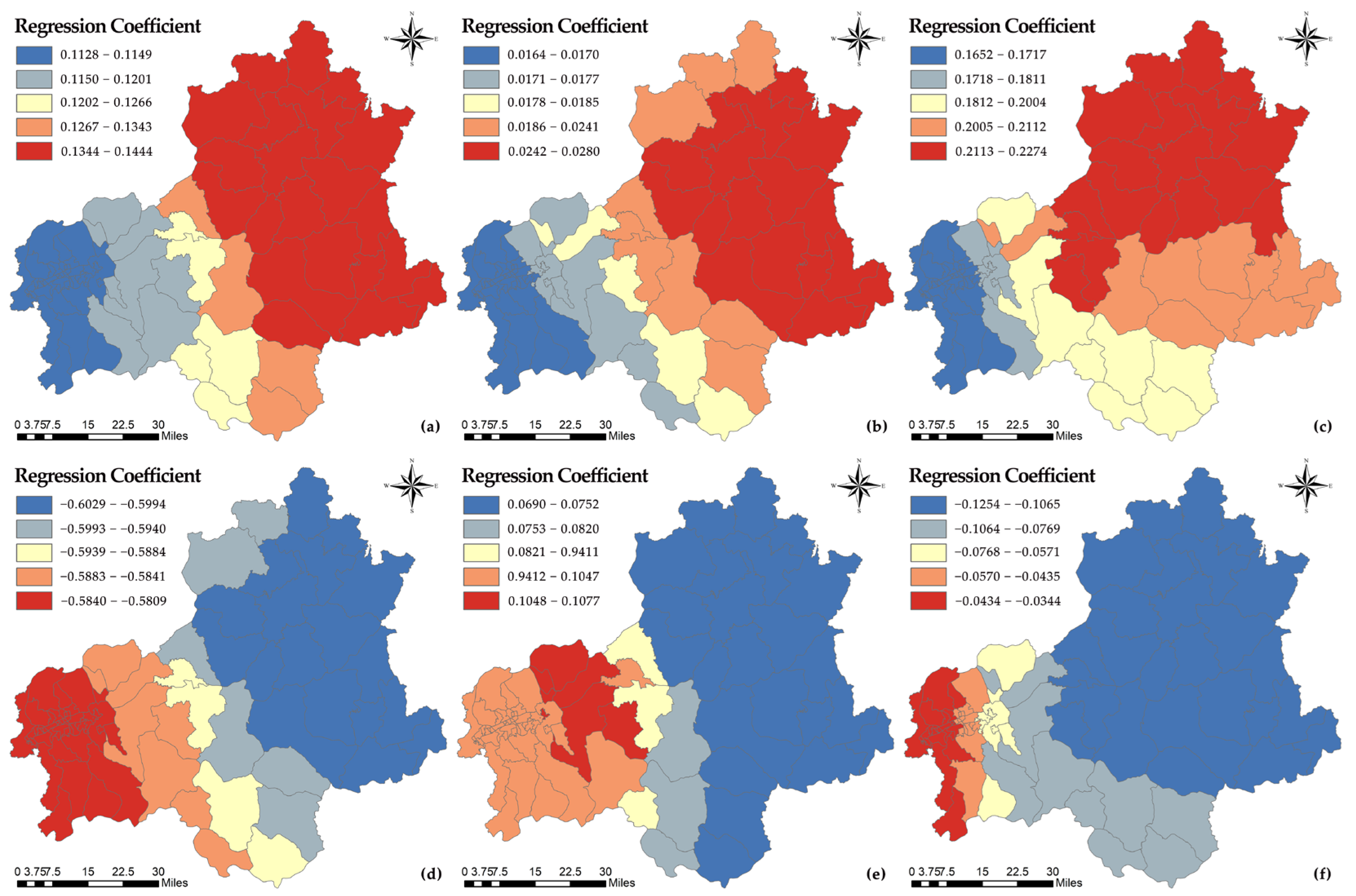
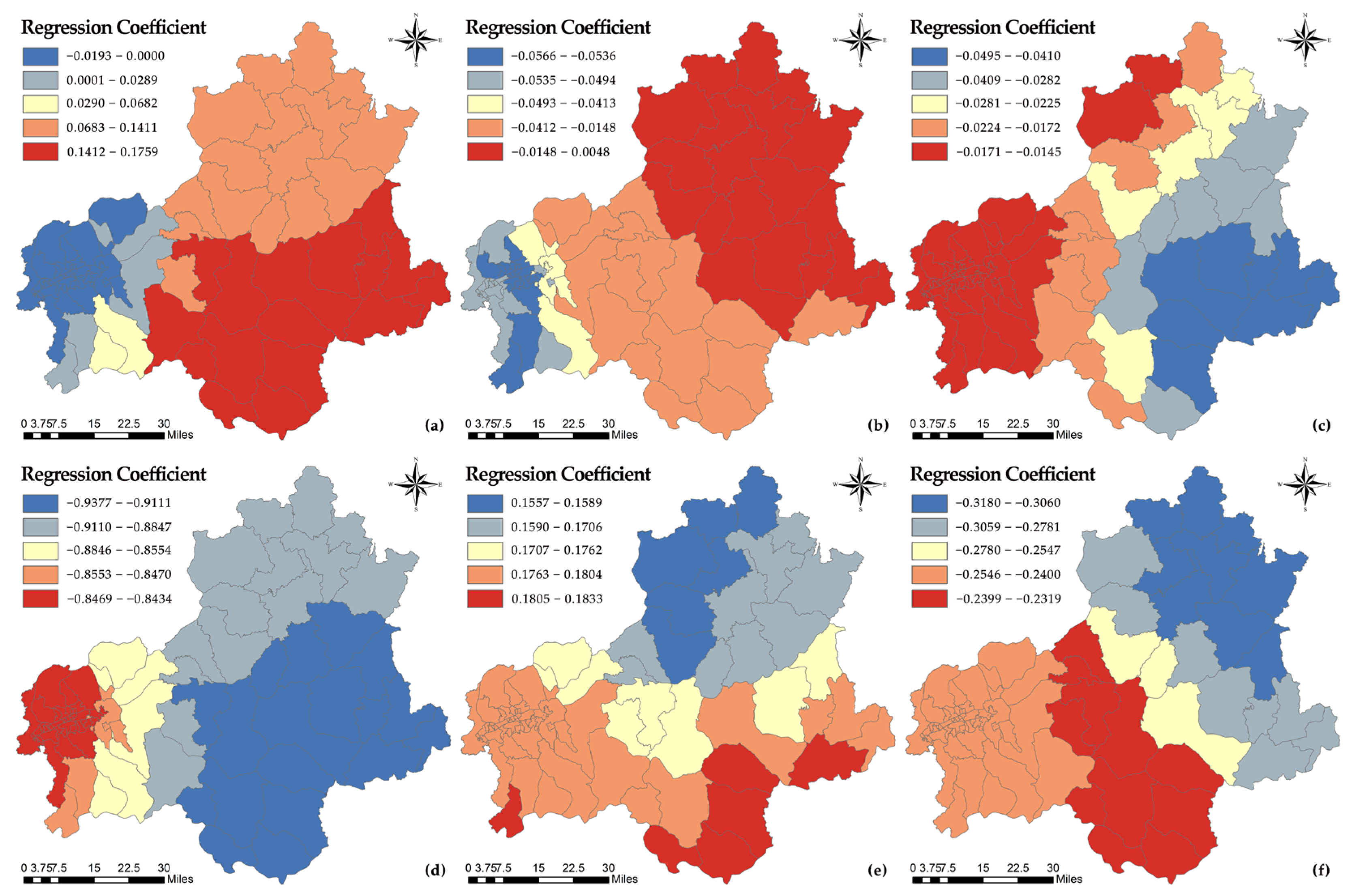
Disclaimer/Publisher’s Note: The statements, opinions and data contained in all publications are solely those of the individual author(s) and contributor(s) and not of MDPI and/or the editor(s). MDPI and/or the editor(s) disclaim responsibility for any injury to people or property resulting from any ideas, methods, instructions or products referred to in the content. |
© 2025 by the authors. Licensee MDPI, Basel, Switzerland. This article is an open access article distributed under the terms and conditions of the Creative Commons Attribution (CC BY) license (https://creativecommons.org/licenses/by/4.0/).