Spatiotemporal Landslide Monitoring in Complex Environments Using Radiative Transfer Model and SBAS-InSAR Technology

 , ,
, ,  , ,
, ,
Abstract
1. Introduction
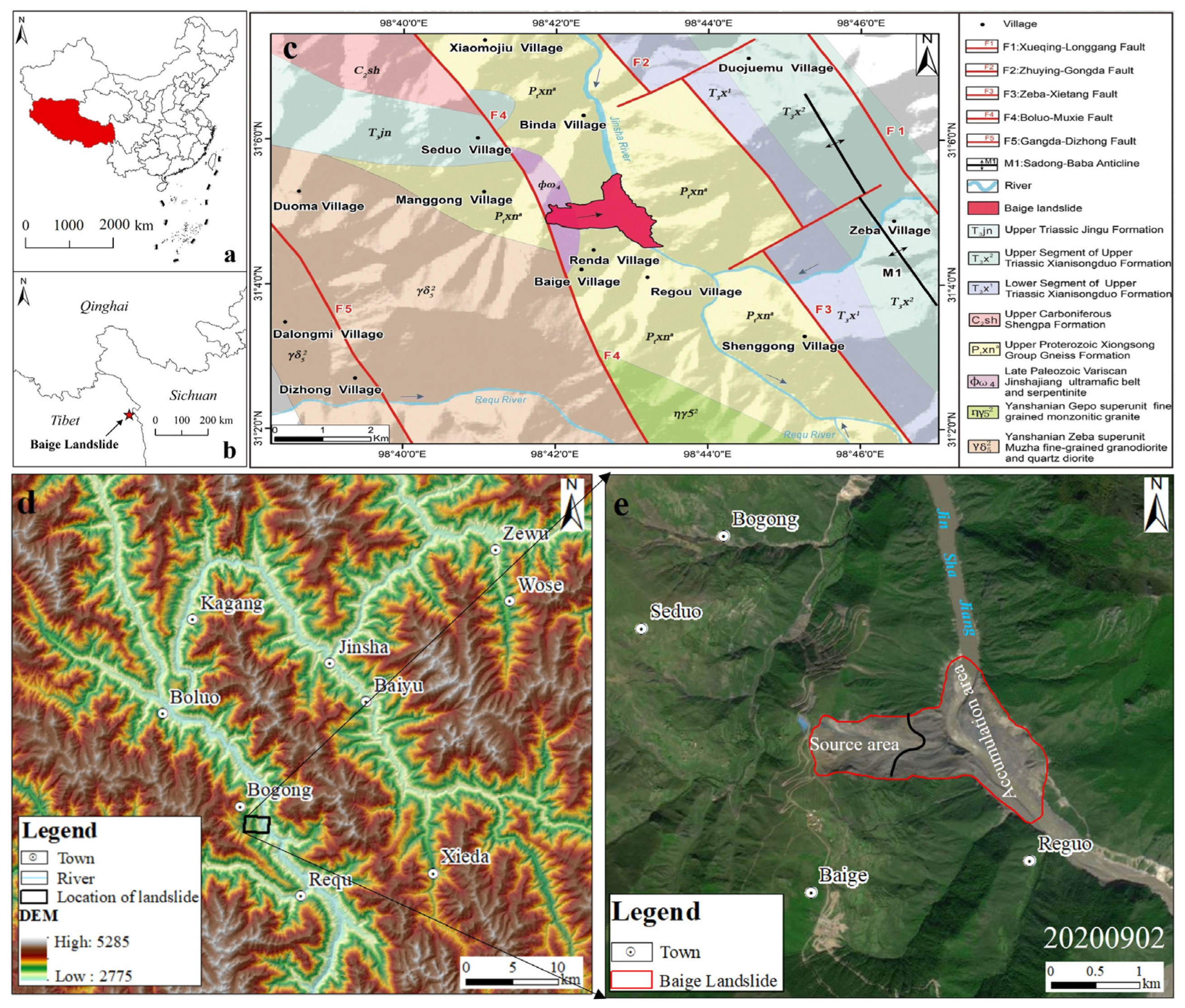
2. Study Area
3. Materials and Methods
3.1. Data
3.1.1. Satellite Remote Sensing Data
3.1.2. Topographical and Geological Data
3.1.3. Precipitation Data
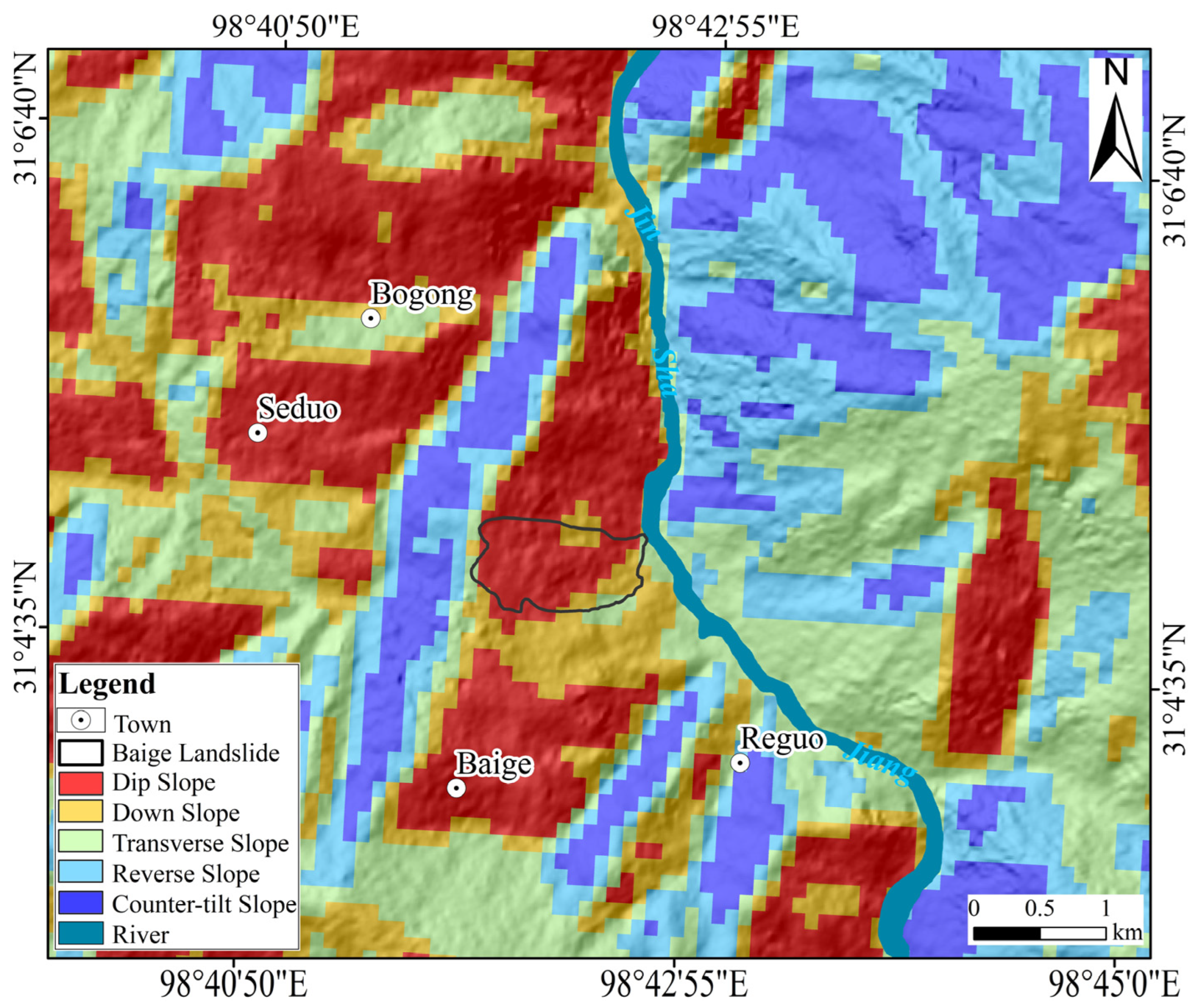
3.2. Classification of Slope Types
3.3. Estimation of CWC Based on the Radiative Transfer Model
3.3.1. Landslide Monitoring Indicator
3.3.2. PROSAIL Model
3.3.3. Sobol Global Sensitivity
3.4. Acquisition of Surface Displacement Based on SBAS-InSAR Technology
4. Results
4.1. Landslide Susceptibility
4.2. CWC Estimation Results
4.2.1. Model Parameter Sensitivity Analysis
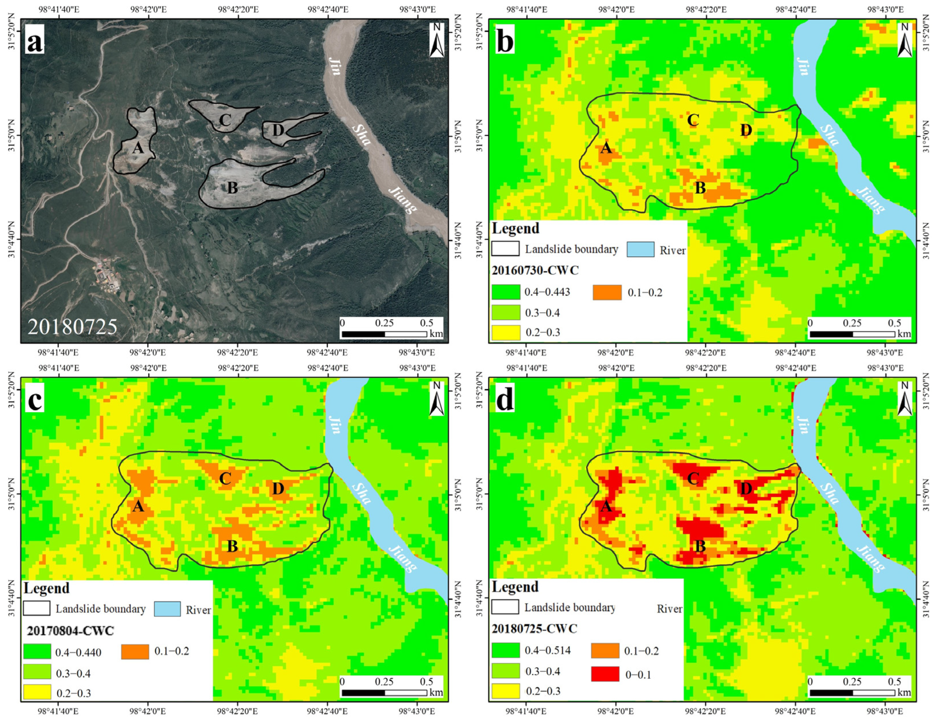
4.2.2. Spatiotemporal Characteristics of Landslide Creep and CWC
4.2.3. Quantitative Analysis of Vegetation Anomaly Pixels
4.3. Surface Deformation Extraction Results
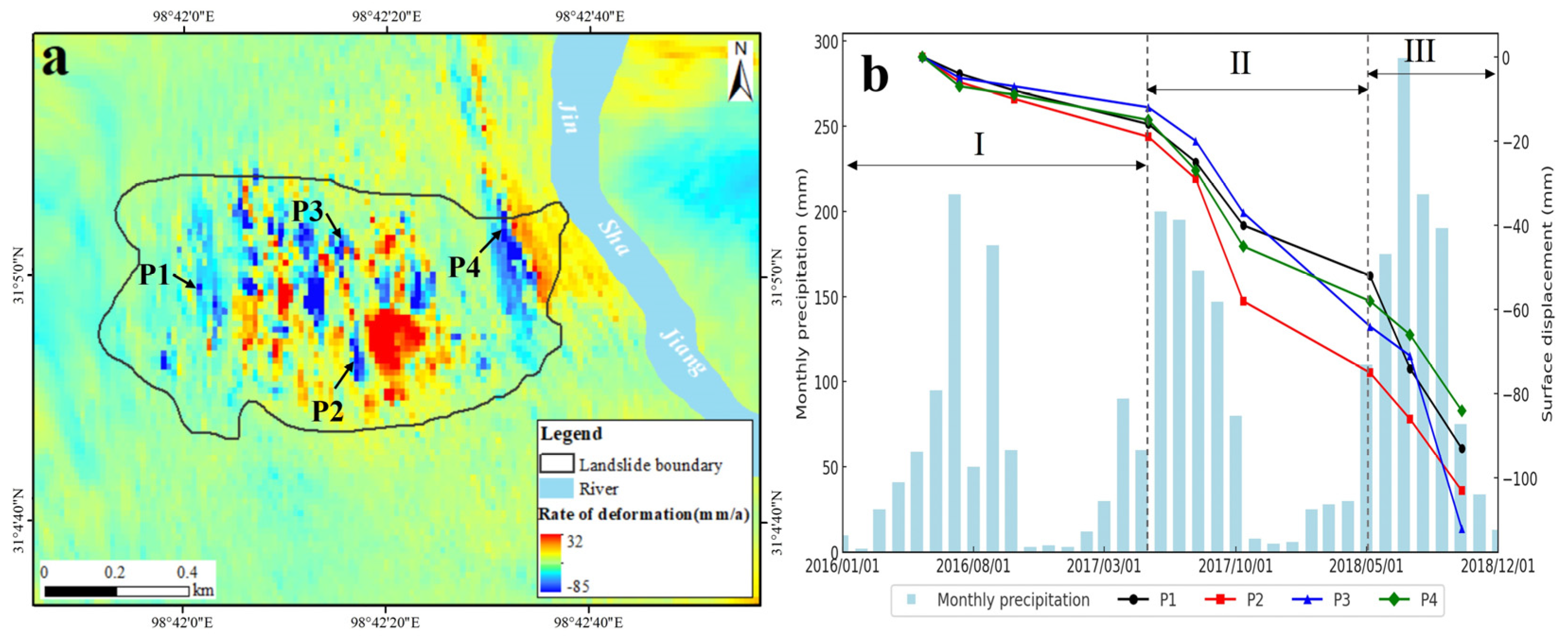
4.3.1. Surface Deformation Analysis
4.3.2. Quantitative Analysis of Surface Deformation
4.4. Analysis of Spatial Variability of Landslide
5. Discussion
5.1. Contributions
5.2. CWC Spatiotemporal Change Impact Factors
6. Conclusions
Author Contributions
Funding
Data Availability Statement
Acknowledgments
Conflicts of Interest
References
- James, N.; Sitharam, T. Assessment of Seismically Induced Landslide Hazard for the State of Karnataka Using GIS Technique. J. Indian Soc. Remote Sens. 2013, 42, 73–89. [Google Scholar] [CrossRef]
- Bogaard, T.; Greco, R. Landslide hydrology: From hydrology to pore pressure. Wiley Interdiscip. Rev. Water 2016, 3, 439–459. [Google Scholar] [CrossRef]
- Xu, Q.; Zhu, X.; Li, W.; Dong, X. Technical progress of space-air-ground collaborative monitoring of landslide. J. Surv. Mapp. 2022, 51, 1416–1436. [Google Scholar] [CrossRef]
- Gao, Y.; Li, B.; Feng, Z.; Zuo, X. Analysis of global climate change and geohazard response. J. Geomech. 2017, 23, 65–77. [Google Scholar] [CrossRef]
- Li, B.; Jenkins, C.; Xu, W. Strategic protection of landslide vulnerable mountains for biodiversity conservation under land-cover and climate change impacts. Proc. Natl. Acad. Sci. USA 2022, 119, e2113416118. [Google Scholar] [CrossRef] [PubMed]
- Kc, R.; Sharma, K.; Dahal, B.K.; Aryal, M.; Subedi, M. Study of the spatial distribution and the temporal trend of landslide disasters that occurred in the Nepal Himalayas from 2011 to 2020. Environ. Earth Sci. 2023, 83, 42. [Google Scholar] [CrossRef]
- Alcántara-Ayala, I.; Sassa, K. Landslide risk management: From hazard to disaster risk reduction. Landslides 2023, 20, 2031–2037. [Google Scholar] [CrossRef]
- Xu, Q.; Dong, X.; Li, W. integrated Space-air-ground early detection, monitoring and warning system for potential catastrophic geohazards. J. Wuhan Univ. (Inf. Sci. Ed.) 2019, 44, 957–966. [Google Scholar] [CrossRef]
- Dai, K.; Deng, J.; Xu, Q.; Li, Z.; Shi, X.; Hancock, C.; Wen, N.; Zhang, L.; Zhuo, G. Interpretation and sensitivity analysis of the InSAR line of sight displacements in landslide measurements. GIScience Remote Sens. 2022, 59, 1226–1242. [Google Scholar] [CrossRef]
- Huang, Y.; Xu, C.; Xue, Z.; Hu, J.; Guo, Y.; Fu, D. A Brief Analysis of Casualty Patterns in Winter Landslide Events: The Zhenxiong 1.22 Landslide Case. Disaster Sci. 2025, 40, 110–116. [Google Scholar] [CrossRef]
- Zheng, G.; Xu, Q.; Liu, X.; Li, Y.; Dong, X.; Ju, N.; Guo, C. Features and Formation Mechanism of the 23 July 2019 Landslide–Debris Flow in Jichang Town, Shuicheng County, Guizhou Province. J. Eng. Geol. 2020, 28, 541–556. [Google Scholar] [CrossRef]
- Liang, J.; Cheng, Y.; Wang, J.; Wang, Y.; Liu, B.; Wang, M.; Yang, L. Remote sensing investigation of the Wulipo mega-landslide disaster in Sanxi Village, Dujiangyan, Sichuan Province, July 10, 2013, and an analysis of the causal mechanism. J. Eng. Geol. 2014, 22, 1194–1203. [Google Scholar] [CrossRef]
- Xu, Q.; Li, W.; Dong, X. Preliminary study on the characteristics and genesis mechanism of landslide in Xinmao Village, Feixi Town, Mao County, Sichuan. J. Rock Mech. Eng. 2017, 36, 2613–2628. [Google Scholar] [CrossRef]
- Ge, D.; Dai, K.; Guo, Z.; Li, Z. Early Identification of Serious Geological Hazards with Integrated Remote Sensing Technologies: Thoughts and Recommendations. J. Wuhan Univ. Inf. Sci. Ed. 2019, 44, 10–14. [Google Scholar] [CrossRef]
- Li, Z.; Zhu, W.; Yu, C.; Zhang, Q.; Zhang, C.; Liu, Z.; Zhang, X.; Chen, B.; Du, J.; Song, C. Interferometric synthetic aperture radar for deformation mapping: Opportunities, challenges and the outlook. J. Surv. Mapp. 2022, 51, 1485–1519. [Google Scholar] [CrossRef]
- Han, W.; Zhang, X.; Wang, Y.; Wang, L.; Huang, X.; Li, J.; Wang, S.; Chen, W.; Li, X.; Feng, R.; et al. A survey of machine learning and deep learning in remote sensing of geological environment: Challenges, advances, and opportunities. ISPRS J. Photogramm. Remote Sens. 2023, 202, 87–113. [Google Scholar] [CrossRef]
- Xu, Z.; Zhang, W.; Zhang, T.; Yang, Z.; Li, J. Efficient Transformer for Remote Sensing Image Segmentation. Remote Sens. 2021, 13, 3585. [Google Scholar] [CrossRef]
- Liu, Z.; Qiu, H.; Zhu, Y.; Liu, Y.; Yang, D.; Ma, S.; Zhang, J.; Wang, Y.; Wang, L.; Tang, B. Efficient Identification and Monitoring of Landslides by Time-Series InSAR Combining Single- and Multi-Look Phases. Remote Sens. 2022, 14, 1026. [Google Scholar] [CrossRef]
- Mondini, A.C.; Guzzetti, F.; Chang, K.-T.; Monserrat, O.; Martha, T.R.; Manconi, A. Landslide failures detection and mapping using Synthetic Aperture Radar: Past, present and future. Earth-Sci. Rev. 2021, 216, 103574. [Google Scholar] [CrossRef]
- Dong, J.; Zhang, L.; Li, M.; Yu, Y.; Liao, M.; Gong, J.; Luo, H. Measuring precursory movements of the recent Xinmo landslide in Mao County, China with Sentinel-1 and ALOS-2 PALSAR-2 datasets. Landslides 2017, 15, 135–144. [Google Scholar] [CrossRef]
- Zhang, L.; Dai, K.; Deng, J.; Ge, D.; Liang, R.; Li, W.; Xu, Q. Identifying Potential Landslides by Stacking-InSAR in Southwestern China and Its Performance Comparison with SBAS-InSAR. Remote Sens. 2021, 13, 3662. [Google Scholar] [CrossRef]
- Xiao, R.; Jiang, M.; Li, Z.; He, X. New insights into the 2020 Sardoba dam failure in Uzbekistan from Earth observation. Int. J. Appl. Earth Obs. Geoinf. 2022, 107, 102705. [Google Scholar] [CrossRef]
- Cigna, F.; Tapete, D. Present-day land subsidence rates, surface faulting hazard and risk in Mexico City with 2014–2020 Sentinel-1 IW InSAR. Remote Sens. Environ. 2021, 253, 112161. [Google Scholar] [CrossRef]
- Hu, X.; Bürgmann, R.; Fielding, E.J.; Lee, H. Internal kinematics of the Slumgullion landslide (USA) from high-resolution UAVSAR InSAR data. Remote Sens. Environ. 2020, 251, 112057. [Google Scholar] [CrossRef]
- Aguemoune, S.; Ayadi, A.; Belhadj-Aissa, A.; Bezzeghoud, M. A novel interpolation method for InSAR atmospheric wet delay correction. J. Appl. Geophys. 2019, 163, 96–107. [Google Scholar] [CrossRef]
- Achache, J.; Fruneau, B.; Delacourt, C. Applicability of SAR Interferometry for Monitoring of Landslides. Proc. Second. ERS Appl. Workshop 1996, 383, 165–168. [Google Scholar]
- Ferretti, A.; Prati, C.; Rocca, F. Permanent Scatterers in SAR Interferometry. Proc. IEEE 2002, 39, 8–20. [Google Scholar] [CrossRef]
- Motagh, M.; Wetzel, H.-U.; Roessner, S.; Kaufmann, H. A TerraSAR-X InSAR Study of Landslides in Southern Kyrgyzstan, Central Asia. Remote Sens. Lett. 2013, 4, 657–666. [Google Scholar] [CrossRef]
- Li, Z.; Song, C.; Yu, C.; Xiao, R.; Chen, L.; Luo, H.; Dai, K.; Ge, D.; Ding, Y.; Zhang, Y.; et al. Application of Satellite Radar Remote Sensing to Landslide Detection and Monitoring Challenges and Solutions. Geomat. Inf. Sci. Wuhan Univ. 2019, 44, 967–979. [Google Scholar] [CrossRef]
- Yue, G.; Liu, Y.; Zheng, C. Research on DEM fusion method of InSAR technology in complex terrain areas. Surv. Mapp. Spat. Geogr. Inf. 2021, 44, 6. [Google Scholar] [CrossRef]
- Deng, J.; Ma, C.; Zhang, Y. Shallow landslide characteristics and its response to vegetation by example of July 2013, extreme rainstorm, Central Loess Plateau, China. Bull. Eng. Geol. Environ. 2022, 81, 100. [Google Scholar] [CrossRef]
- Li, M.; Ma, C.; Du, C.; Yang, W.; Lyu, L.; Wang, X. Landslide response to vegetation by example of July 25–26, 2013, extreme rainstorm, Tianshui, Gansu Province, China. Bull. Eng. Geol. Environ. 2020, 80, 751–764. [Google Scholar] [CrossRef]
- Zhang, J.; Qiu, H.; Tang, B.; Yang, D.; Liu, Y.; Liu, Z.; Ye, B.; Zhou, W.; Zhu, Y. Accelerating Effect of Vegetation on the Instability of Rainfall-Induced Shallow Landslides. Remote Sens. 2022, 14, 5743. [Google Scholar] [CrossRef]
- Wang, H.; Guo, Q.; Ge, X.; Tong, L. A Spatio-Temporal Monitoring Method Based on Multi-Source Remote Sensing Data Applied to the Case of the Temi Landslide. Land 2022, 11, 1367. [Google Scholar] [CrossRef]
- Guo, X.; Guo, Q.; Feng, Z. Detecting the Vegetation Change Related to the Creep of 2018 Baige Landslide in Jinsha River, SE Tibet Using SPOT Data. Front. Earth Sci. 2021, 9, 706998. [Google Scholar] [CrossRef]
- Saito, H.; Uchiyama, S.; Teshirogi, K. Rapid vegetation recovery at landslide scars detected by multitemporal high-resolution satellite imagery at Aso volcano, Japan. Geomorphology 2022, 398, 107989. [Google Scholar] [CrossRef]
- Wang, B.; He, L.; He, Z.; Qu, R.; Kang, G. Study of early identification method for large landslides in high vegetation coverage areas of Southwest China. Front. Ecol. Evol. 2023, 11, 1169028. [Google Scholar] [CrossRef]
- Bao, Y.; Su, L.; Chen, J.; Ouyang, C.; Yang, T.; Lei, Z.; Li, Z. Dynamic process of a high-level landslide blocking river event in a deep valley area based on FDEM-SPH coupling approach. Eng. Geol. 2023, 319, 107108. [Google Scholar] [CrossRef]
- Li, F.; Fu, J.; Cheng, X.; Zheng, X.; Hu, J.; Jiang, N.; Chen, Z.; Zheng, P.; Zhang, S. A Study on the Differences in Vegetation Carbon Content between the Upper Reaches of the Jinsha River and Other Typical Watersheds. Technol. Econ. Change 2024, 8, 11–18. [Google Scholar] [CrossRef]
- Ouyang, C.; An, H.; Zhou, S.; Wang, Z.; Su, P.; Wang, D.; Cheng, D.; She, J. Insights from the failure and dynamic characteristics of two sequential landslides at Baige village along the Jinsha River, China. Landslides 2019, 16, 1397–1414. [Google Scholar] [CrossRef]
- Fan, X.; Yang, F.; Siva Subramanian, S.; Xu, Q.; Feng, Z.; Mavrouli, O.; Peng, M.; Ouyang, C.; Jansen, J.D.; Huang, R. Prediction of a multi-hazard chain by an integrated numerical simulation approach: The Baige landslide, Jinsha River, China. Landslides 2019, 17, 147–164. [Google Scholar] [CrossRef]
- Wen, B.; Zeng, Q.; Yan, T. A preliminary geomechanical model for the initiation of large rocky, high-speed remote landslides on the southeastern Qinghai-Tibet Plateau. Eng. Sci. Technol. 2020, 52, 38–49. [Google Scholar] [CrossRef]
- Chen, Q.; Wu, H.; Zhang, M.; Yang, L. Research on the Mechanism of Earthquake-triggered Failure of Bedding Slope in Taxian of Xinjiang. Saf. Environ. Eng. 2021, 28, 88–95. [Google Scholar] [CrossRef]
- Zeng, Y.; Hao, D.; Huete, A.; Dechant, B.; Berry, J.; Chen, J.M.; Joiner, J.; Frankenberg, C.; Bond-Lamberty, B.; Ryu, Y.; et al. Optical vegetation indices for monitoring terrestrial ecosystems globally. Nat. Rev. Earth Environ. 2022, 3, 477–493. [Google Scholar] [CrossRef]
- Hotta, W.; Morimoto, J.; Yanai, S.; Uchida, Y.; Nakamura, F. Environmental heterogeneity on landslide slopes affects the long-term recoveries of forest ecosystem components. Catena 2024, 234, 107578. [Google Scholar] [CrossRef]
- Lyons, D.S.; Dobrowski, S.Z.; Holden, Z.A.; Maneta, M.P.; Sala, A. Soil moisture variation drives canopy water content dynamics across the western U.S. Remote Sens. Environ. 2021, 253, 112233. [Google Scholar] [CrossRef]
- Ceccato, P.; Gobron, N.; Flasse, S.p.; Pinty, B.; Tarantola, S. Designing a spectral index to estimate vegetation water content from remote sensing data: Part 1 Theoretical approach. Remote Sens. Environ. 2002, 82, 188–197. [Google Scholar] [CrossRef]
- Yin, S.; Zhou, K.; Cao, L.; Shen, X. Estimating the Horizontal and Vertical Distributions of Pigments in Canopies of Ginkgo Plantation Based on UAV-Borne LiDAR, Hyperspectral Data by Coupling PROSAIL Model. Remote Sens. 2022, 14, 715. [Google Scholar] [CrossRef]
- Wang, L.; Chen, S.; Peng, Z.; Huang, J.; Wang, C.; Jiang, H.; Zheng, Q.; Li, D. Phenology Effects on Physically Based Estimation of Paddy Rice Canopy Traits from UAV Hyperspectral Imagery. Remote Sens. 2021, 13, 1792. [Google Scholar] [CrossRef]
- Baret, F.; Fourty, T. Estimation of leaf water content and specific leaf weight from reflectance and transmittance measurements. Agronomie 1997, 17, 455–464. [Google Scholar] [CrossRef]
- Verhoef, W. Light Scattering by Leaf Layers with Application to Canopy Reflectance Modeling: The SAIL Model. Remote Sens. Environ. 1984, 16, 125–141. [Google Scholar] [CrossRef]
- Han, Y.; Dong, Y.; Zhu, Y.; Huang, W. Remote Sensing Inversion of Vegetation Parameters with IPROSAIL-Net. IEEE Trans. Geosci. Remote Sens. 2024, 62, 1–16. [Google Scholar] [CrossRef]
- Zhang, X.; Jiao, Z.; Zhao, C.; Yin, S.; Cui, L.; Dong, Y.; Zhang, H.; Guo, J.; Xie, R.; Li, S.; et al. Retrieval of Leaf Area Index by Linking the PROSAIL and Ross-Li BRDF Models Using MODIS BRDF Data. Remote Sens. 2021, 13, 4911. [Google Scholar] [CrossRef]
- Sobol, I.M. Global sensitivity indices for nonlinear mathematical models and their Monte Carlo estimates. Math. Comput. Simul. 2001, 55, 271–280. [Google Scholar] [CrossRef]
- Berardino, P.; Fornaro, G.; Lanari, R.; Sansosti, E. A new algorithm for surface deformation monitoring based on small baseline differential SAR interferograms. IEEE Trans. Geosci. Remote Sens. 2002, 40, 2375–2383. [Google Scholar] [CrossRef]
- Tao, Q.; Wang, F.; Guo, Z.; Hu, L.; Yang, C.; Liu, T. Accuracy verification and evaluation of small baseline subset (SBAS) interferometric synthetic aperture radar (InSAR) for monitoring mining subsidence. Eur. J. Remote Sens. 2021, 54, 642–663. [Google Scholar] [CrossRef]
- Zhang, P.; Guo, Z.; Guo, S.; Xia, J. Land Subsidence Monitoring Method in Regions of Variable Radar Reflection Characteristics by Integrating PS-InSAR and SBAS-InSAR Techniques. Remote Sens. 2022, 14, 3265. [Google Scholar] [CrossRef]
- Yang, C.; Zhang, T.; Gao, G. Application of SBAS-InSAR technology in monitoring of ground deformation of representative giant landslides in Jinsha river basin, Jiangda County, Tibet. Chin. J. Geol. Hazard Control. 2022, 33, 94–105. [Google Scholar] [CrossRef]
- Chai, B.; Yin, K. Influence of inclination of rock strata and angle of slope direction on slope stability of downslope. J. Rock Mech. Eng. 2009, 28, 7. [Google Scholar] [CrossRef]
- Chen, G.; Cheng, G.; Peng, S.; Zhang, W.; Wang, L. Regional landslide susceptibility evaluation based on geomorphology–slope-structure slope unit delineation. Geol. Rev. 2024, 70, 5. [Google Scholar] [CrossRef]
- Ma, C.; Miao, H.; Yang, B. Analysis of small temporal deformations and disaster time forecasting of large landslides based on SBAS-InSAR technology. Sci. Technol. Eng. 2023, 23, 9404–9412. [Google Scholar] [CrossRef]
- Guo, W.; Chen, Z.; Wang, W.; Gao, W.; Guo, M.-m.; Kang, H.; Li, P.; Wang, W.; Zhao, M. Telling a different story: The promote role of vegetation in the initiation of shallow landslides during rainfall on the Chinese Loess Plateau. Geomorphology 2020, 350, 106879. [Google Scholar] [CrossRef]
- Huang, F.; Chen, J.; Liu, W.; Huang, J.; Hong, H.; Chen, W. Regional rainfall-induced landslide hazard warning based on landslide susceptibility mapping and a critical rainfall threshold. Geomorphology 2022, 408, 108236. [Google Scholar] [CrossRef]
- Zhang, K.; Wang, S.; Bao, H.; Zhao, X. Characteristics and influencing factors of rainfall-induced landslide and debris flow hazards in Shanxi Province, China. Nat. Hazards Earth Syst. Sci. 2019, 19, 93–105. [Google Scholar] [CrossRef]
- Naghdi, R.; Maleki, S.; Abdi, E.; Gholami, M. Assessing the Effect of Alnus Roots on Hillslope Stability for Application in Soil Bioengineering. J. For. Sci. 2013, 59, 417–423. [Google Scholar] [CrossRef]
- Pollen, N. Temporal and Spatial Variability in Root Reinforcement of Streambanks: Accounting for Soil Shear Strength and Moisture. Catena 2007, 69, 197–205. [Google Scholar] [CrossRef]
- Yang, W.; Qi, W.; Zhou, J. Effects of Precipitation and Topography on Vegetation Recovery at Landslide Sites after the 2008 Wenchuan Earthquake. Land Degrad. Dev. 2018, 29, 3355–3365. [Google Scholar] [CrossRef]
- Deijns, A.A.J.; Bevington, A.R.; van Zadelhoff, F.; de Jong, S.M.; Geertsema, M.; McDougall, S. Semi-Automated Detection of Landslide Timing Using Harmonic Modelling of Satellite Imagery, Buckinghorse River, Canada. Int. J. Appl. Earth Obs. Geoinf. 2020, 84, 101943. [Google Scholar] [CrossRef]


| Image Parameter | Sentinel-2 for Monitoring Vegetation Changes | Sentinel-1 for Monitoring Landslide Displacement |
|---|---|---|
| Wave Band | Band1~7, Band8A, Band8(NIR), Band9~12 | C |
| Imaging Mode | MSI | IW |
| Data Products | L1C, L2A | SLC |
| Polarisation Pattern | / | VV |
| Spatial Resolution/m | 10, 20, 60 | 5 × 20 |
| Revisit Cycle/d | 10 | 12 |
| Image Time | 30 July 2016, 4 August 2017, 5 June 2018, 25 July 2018 | 2016–2018 |
| Parameter | Range | Step Size |
|---|---|---|
| Leaf structure (N) | 1.5 | - |
| Chlorophyll content (Cab) | 40 μg/cm2 | - |
| Equivalent Water Thickness (EWT) | 0.007–0.05 | 0.002 |
| Leaf Area Index (LAI) | 2–6 | 0.02 |
| Dry matter content (Cm) | 0.018–0.02 g/cm2 | 0.002 |
| Carotenoid content (Car) | 20 g/cm2 | - |
| Observed azimuth angle () | 0° | - |
| Solar zenith angle () | 20° | - |
| Soil moisture ratio (Psoil) | 0.2 | - |
| Hot spot factor (Hspot) | 0.003 | - |
| Average leaf inclination angle (ALIA) | 40° | - |
| 30 July 2016 | 4 August 2017 | 25 July 2018 | ||||
|---|---|---|---|---|---|---|
| Pixel | Percentage | Pixel | Percentage | Pixel | Percentage | |
| A(CWC < 0.04) | 64 | 32% | 146 | 73% | 153 | 76.5% |
| B(CWC < 0.04) | 187 | 62.3% | 194 | 64.7% | 220 | 73.3% |
| C(CWC < 0.04) | 8 | 6.8% | 87 | 74.4% | 95 | 81.2% |
| D(CWC < 0.04) | 12 | 7.5% | 68 | 42.5% | 81 | 50.6% |
Disclaimer/Publisher’s Note: The statements, opinions and data contained in all publications are solely those of the individual author(s) and contributor(s) and not of MDPI and/or the editor(s). MDPI and/or the editor(s) disclaim responsibility for any injury to people or property resulting from any ideas, methods, instructions or products referred to in the content. |
© 2025 by the authors. Licensee MDPI, Basel, Switzerland. This article is an open access article distributed under the terms and conditions of the Creative Commons Attribution (CC BY) license (https://creativecommons.org/licenses/by/4.0/).
Share and Cite
Wang, B.; He, L.; He, Z.; Song, Y.; Qu, R.; Hu, J.; Wang, Z.; Zhang, Z. Spatiotemporal Landslide Monitoring in Complex Environments Using Radiative Transfer Model and SBAS-InSAR Technology. Land 2025, 14, 956. https://doi.org/10.3390/land14050956
Wang B, He L, He Z, Song Y, Qu R, Hu J, Wang Z, Zhang Z. Spatiotemporal Landslide Monitoring in Complex Environments Using Radiative Transfer Model and SBAS-InSAR Technology. Land. 2025; 14(5):956. https://doi.org/10.3390/land14050956
Chicago/Turabian StyleWang, Bing, Li He, Zhengwei He, Yongze Song, Rui Qu, Jiao Hu, Zhifei Wang, and Zehua Zhang. 2025. "Spatiotemporal Landslide Monitoring in Complex Environments Using Radiative Transfer Model and SBAS-InSAR Technology" Land 14, no. 5: 956. https://doi.org/10.3390/land14050956
APA StyleWang, B., He, L., He, Z., Song, Y., Qu, R., Hu, J., Wang, Z., & Zhang, Z. (2025). Spatiotemporal Landslide Monitoring in Complex Environments Using Radiative Transfer Model and SBAS-InSAR Technology. Land, 14(5), 956. https://doi.org/10.3390/land14050956