The first set of results is for the unconstrained and homogeneous landscape when first the property rights belong to the GM producers and the second for when the property rights belong to the non-GM producers. The second set of results are for the heterogeneous landscape.
3.1. The Homogeneous and Unconstrained Landscape
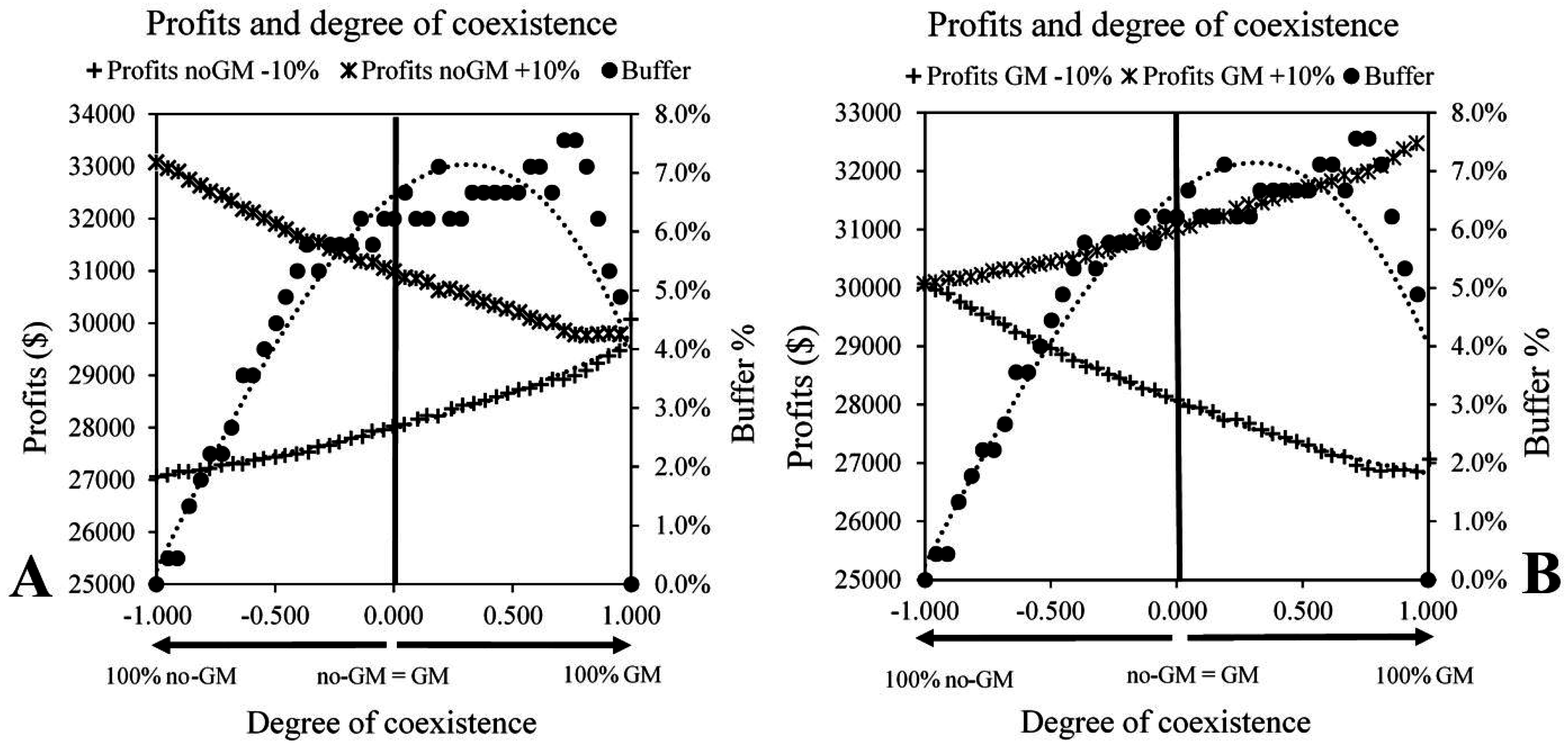
Figure 2 shows in the graph to the left the amount of the profits for the entire landscape and the amount of buffer needed for the non-GM portion of the landscape to be cross-pollinated below the 0.9% threshold when GM producers have the property rights. Represented in the graph are all the intermediate situations between a landscape grown with only the GM crop, or only the non-GM crop.
It can be observed that the percentage of buffer varies from a minimum of 0% (in case of no coexistence in place) to a maximum of 7.8% of the entire landscape. For the situation in which the amount of GM crop equals the amount of non-GM crop (maximum coexistence), the buffer needed to prevent cross-pollination to the threshold level is around 6% of the whole landscape surface. The amount of buffers starts to decline when the GM crop covers around 75% of the landscape due to increasing saturation. The reduction in the surface of the non-GM crop results in a reduction on the length of the edge delimiting the two crops, which translates into a decrease in the surface needed to reduce cross-pollination. The non-GM crop cannot be grown on the landscape when the GM crop covers about 93% of the available surface. The amount of buffer needed to prevent cross-pollination is unrelated to the profitability levels of the crops, and only depends on the specific maximum level of cross-pollination allowed.
With regard to the profits for the entire landscape, when non-GM profitability is 10% higher than GM, an increase in the GM surface causes a reduction in profits whose maximum value is $33,000. When there is the maximum degree of coexistence, which is the value of 0 on the horizontal axis at the center of the graph, profits for the landscape are about $31k, or $2,000 below the profits in the case of full adoption of the non-GM crop. When non-GM profitability is 10% lower than GM profitability, the economic value of the crops on the landscape varies from about $27k to about $30k. When there is the maximum degree of coexistence, the value of both crops on the landscape at $28k is about $1,900 lower than in the case of full adoption of the GM crop on the entire landscape at $29.9k.
Figure 2 also illustrates in the graph to the right the buffer areas in relation to the coexistence between the GM and the non-GM crop on the landscape, and the profits at the landscape level when the GM crop is 10% less or more profitable than the non-GM crop when the non-GM producers have the property rights. The amount of buffer needed for avoiding cross-pollination greater than the 0.9% threshold is not influenced by either the property right assignment or the profitability levels of GM and non-GM crops. The model minimizes the amount of buffer to minimize the economic losses that the buffers cause. Since the profitability of buffers is always modeled as lower than both the GM and the non-GM crop, buffers will always be minimized.
As for the economic returns at the landscape level, they vary from a value of around $30k (100% no-GM) to a maximum of a little under $33 k (100% GM in case of GM 10% more profitable than non-GM), and to a minimum of about $26.9k (100% GM in case of GM 10% less profitable than non-GM). The landscape profits when the maximum degree of coexistence is observed (GM area = non-GM area) vary from a little above $28k to a little below $31k based on the relative profitability between the GM and the non-GM crop.
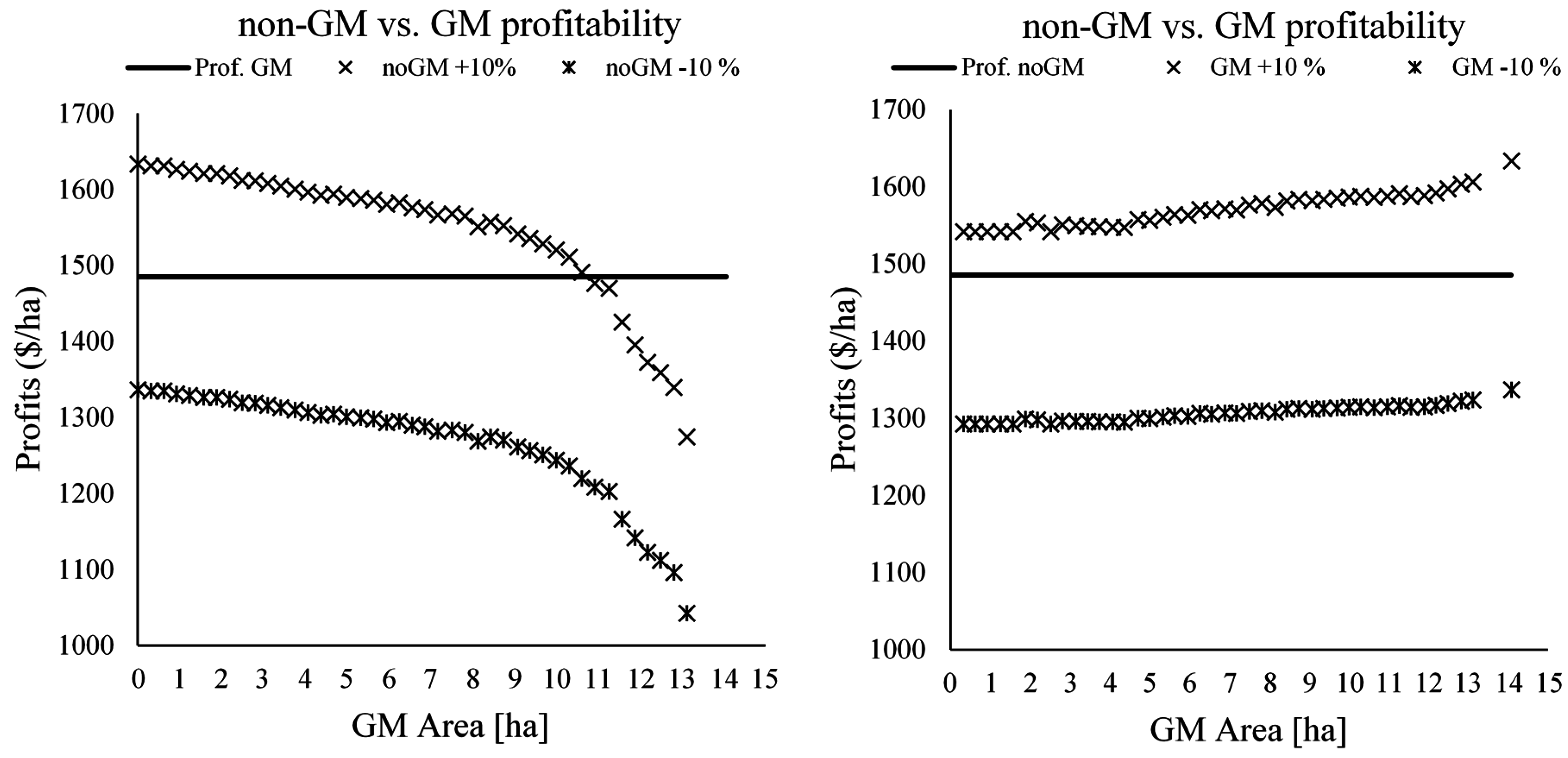
Figure 3 indicates that when the non-GM crop is 10% more profitable than the GM crop, there is an economic incentive to grow the non-GM crop until the GM area equals around 11 hectares. For bigger GM areas the higher non-GM profitability does not allow for covering the costs of creating buffers. The horizontal line is the $1485 per hectare that indicates the baseline economic profit obtained from growing only one type of crop on the landscape. In the −10% profitability scenario for the non-GM crop, coexistence is observed if the competitive advantage for non-GM producers is between $150/ha (or $1485–$1335) to about $360/ha (or $1485–$1125) depending on the amount of GM land on the landscape.
Figure 3 also shows in the graph to the right the per hectare profit of the GM crop in comparison to the non-GM crop taking into account the costs for meeting the 0.9% cross-pollination threshold and as a function of the GM area on the landscape when non-GM producers have the property rights. Since GM producers have to bear the costs of preventing cross-pollination and buffers vary as the GM area varies, GM profitability also changes, while the non-GM profitability remains constant. GM profitability increases as the GM area increases, and the magnitude of the increase is about $60/ha in the case where GM is 10% more profitable than non-GM (from $1,550/ha to $1,610/ha), and about $30/ha in the case where GM is 10% less profitable than non-GM (from $1,300/ha to $1,330/ha). In the case where coexistence is observed and GM is 10% more profitable than non-GM, non-GM producers have a competitive unobserved advantage that varies from $50/ha (or $1,535–$1,485) to about $110/ha (or $1,595–$1,485) based on the amount of the GM crop on the landscape. On the other hand, when GM is 10% less profitable than non-GM and coexistence is observed, GM farmers have a competitive advantage that varies from $180 (or $1,485–$1,305) to $200/ha (or $1,485–$1,285) based on the amount of GM land, with the more GM land on the landscape the less the competitive advantage.
3.2. The Heterogeneous Landscape
Table 4 shows the profits and losses at the landscape level as a function of increasing profitability for the non-GM crop in comparison to the GM crop and thresholds of cross-pollination when GM producers have the property rights.
GM land is constrained so that fields do not switch into a more profitable non-GM crop. One explanation for the constraint that the GM crop is grown despite lower profits may be unobserved competitive advantage for those fields to remain in GM production. Stricter thresholds result in greater economic losses. A threshold of 0.1% implies that there is no economic incentive for growing the non-GM crop even in the event that it is 25% more profitable than the non-GM. For the legislative threshold adopted in the European Union, coexistence becomes profitable when the non-GM crop is between 15% and 20% more profitable than the GM one. When the non-GM crop is 5% more profitable than the GM crop, a threshold of 5% still results in coexistence on the landscape which is less profitable than the baseline. It is possible to quantify what competitive advantage non-GM farms need to have in order to keep growing the non-GM crop. In the case where the non-GM crop is 15% more profitable than the GM one and a 0.10% threshold is in place, coexistence is only possible if non-GM farms have a competitive advantage that is at least sufficient to balance the 4.1% loss. If coexistence is observed on the landscape for all positive values in
Table 4, GM farmers have a competitive advantage in relation to non-GM farmers.
Table 4 also shows the percentage deviation from the baseline of overall economic returns on the landscape in the case where property rights are assigned to non-GM producers, and buffers are created into GM fields. As in the alternative property right scenario, tighter thresholds result in increasing economic losses. At the 0.9% threshold coexistence becomes profitable when the GM crop is between 10% and 15% more profitable than non-GM crops, and at the 0.1% threshold coexistence becomes profitable when the GM crop is between 20% and 25% more profitable than the non-GM crop. For allowing economic coexistence, a threshold higher than 5% should be in place when the non-GM crop is 5% more profitable than the alternative non-GM crop. For all combinations characterized by negative values, a competitive advantage for GM farms is assumed to be in place if coexistence exists on the landscape.
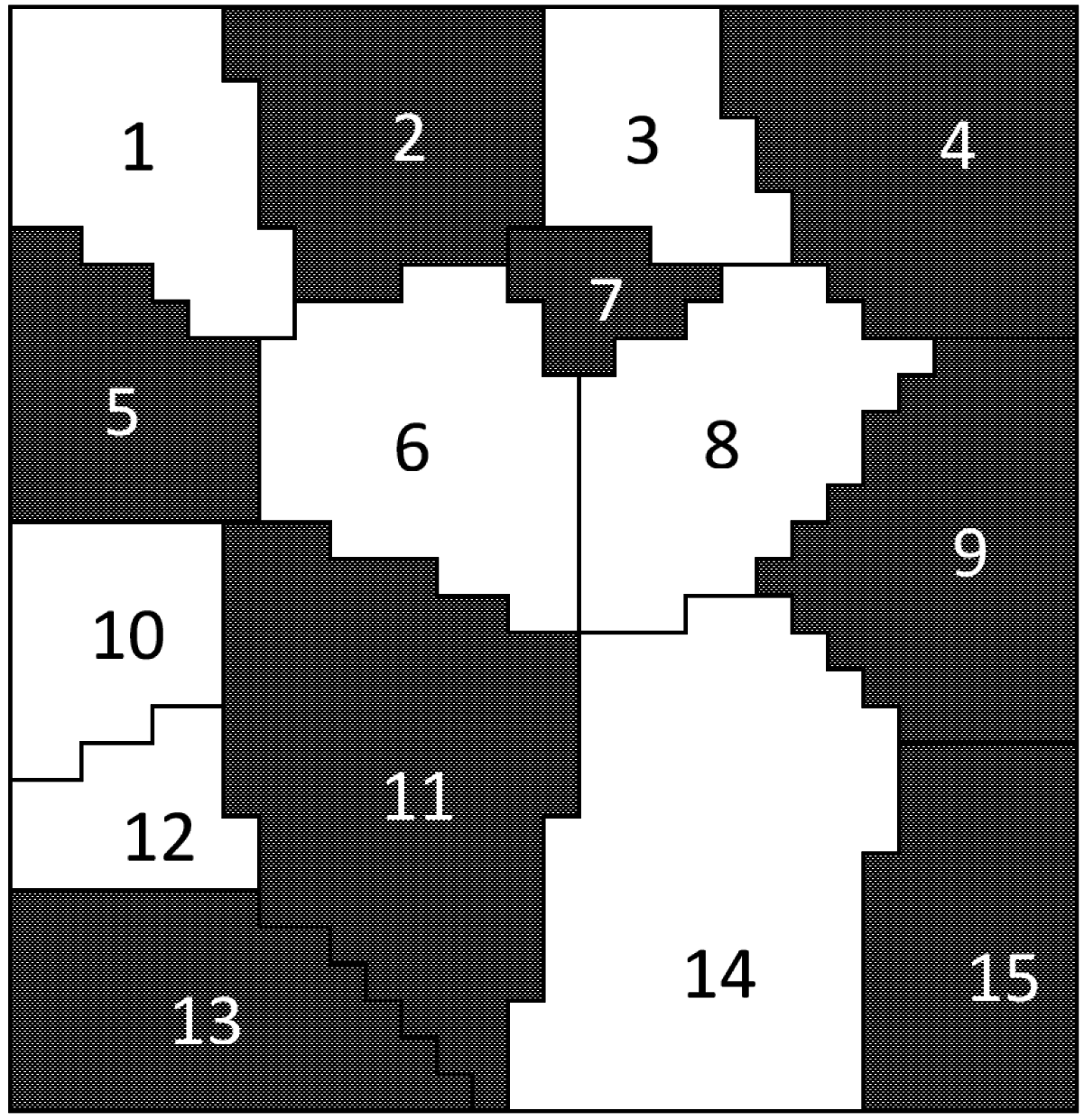
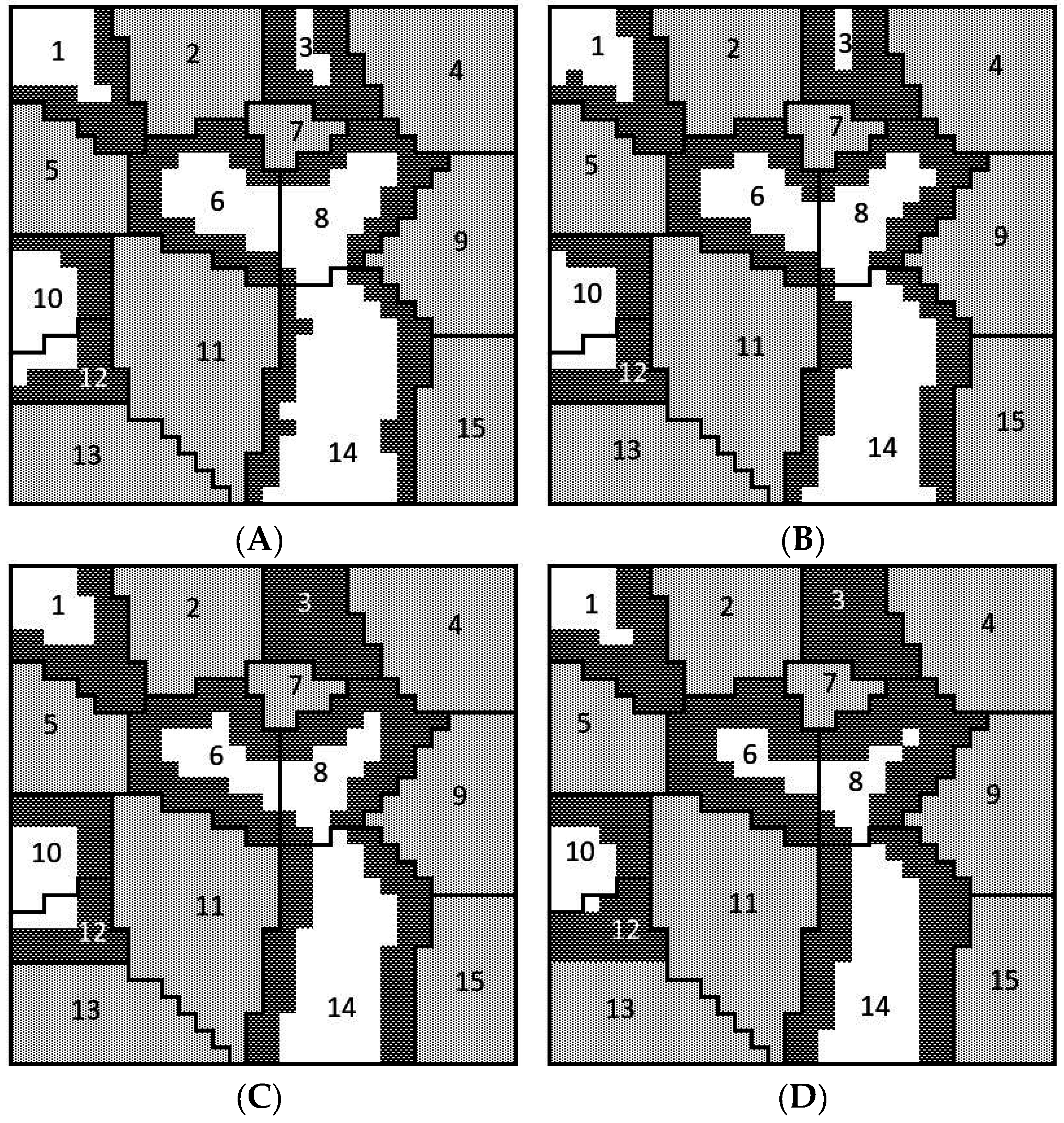
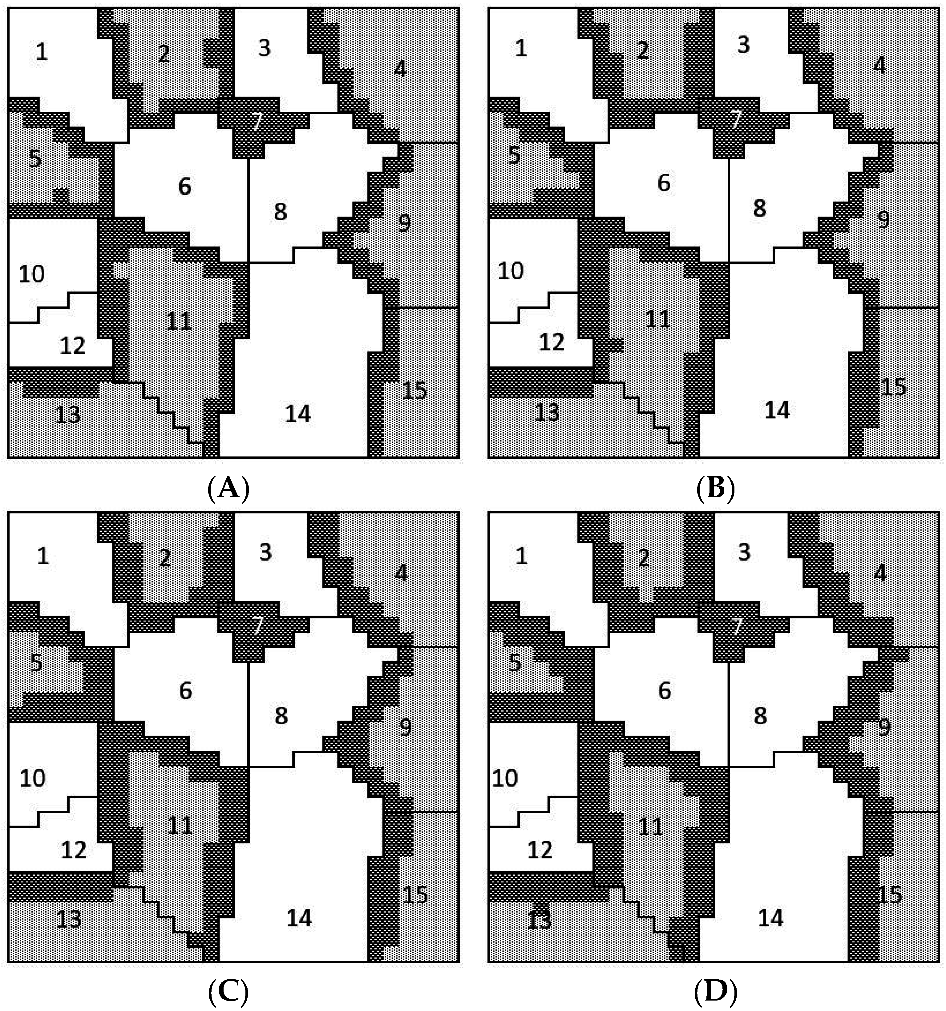
Figure 4 shows the spatial configurations of GM, non-GM, and buffer areas resulting from the model runs for the 5%, 1.5%, 0.9%, and 0.25% thresholds.
Buffers are created inside the non-GM fields because GM producers have the property rights, and increasing buffers result from stricter thresholds of cross-pollination. It is worth noting that buffers do not represent uniformly wide areas that separate GM from non-GM fields, but they are areas that, due to their particular position, and degree of reduced cross-pollination as a function of their position, determine an overall cross-pollination in all the remaining non-GM area lower than the set thresholds of cross-pollination. The buffers absorb most of the pollen that drifts from the nearby GM fields, and this allows the non-buffer portion of the non-GM field to meet the regulatory threshold. This is why thicker buffers are needed when the regulatory threshold is more stringent.
Figure 5 shows the spatial configurations of GM, non-GM, and buffer areas as resulting from the model runs for the 5%, 1.5%, 0.9%, and 0.25% thresholds.
Buffers are in this case created inside GM fields. As in the previous case, the most efficient configurations result in buffers that are not homogeneous in their width. The overall amount of buffer areas increases as a consequence of increasingly strict thresholds of cross-pollination. When GM producers hold the property rights, a buffer area of 11.4% of the total landscape is needed at the least stringent threshold of 5%, and these numbers increase to 30.5% in the case of the most stringent threshold of 0.25%. At the 0.1% threshold the amount of land that can be considered non-GM is lower than the amount of buffer to prevent excessive cross-pollination in the non-GM area. At the 0.9% threshold there is an almost equal amount of non-GM and buffer land. In the case where non-GM producers have the property rights, again the amount of buffer needed to prevent cross-pollination increases the more stringent the thresholds become. In particular, buffers range from 9.5% of the landscape surface at the 5% threshold to 25.4% of the landscape surface in case of a 0.1% threshold of cross-pollination. The differences in percentages of buffers for the two alternative property right assignments arise from the particular landscape configuration, the relative size between GM and non-GM fields, and the overall GM area vs. non-GM area on the landscape.
Table 5 shows the percentage profits relative to the baseline as a function of thresholds of cross-pollination and relative profitability between the GM and the non-GM crop at the field level. This allows for the identification of spatial differences in economic returns from heterogeneity of the fields on the landscape based on field shape, size, and position in space. Due to the property right arrangements, it is assumed that GM fields have homogeneous profitability that is not affected by space, whereas heterogeneity is expected for non-GM fields because buffers are made in the non-GM fields to meet the regulatory threshold of cross-pollination.
Due to computational complexity of the model, it is only possible to elicit when a field is suitable or not for non-GM crops, and all the negative values (represented with dashes in the table) only indicate the spatial economic unsuitability for the non-GM crop. In fact, due to spatial inter-relations of pollen dispersal between fields, it is impossible to derive that, whenever a field is not suitable for the non-GM crop, it is economically better for the GM alternative. This is because switching a field from non-GM to GM will affect the profitability of all neighboring non-GM fields that will require additional buffers that were not required before. A switch of one field from non-GM to GM could even result in the consequential disappearance of all non-GM fields on the landscape.
The results show that fields 14 and 10 are the most suitable for coexistence, whereas field 3 is the least suitable. In particular, field 14 is the largest among the non-GM fields, whereas field 10 borders with one GM field and with the edge of the area created. It therefore receives cross-pollination only from two edges. For field 3, the costs of creating buffers can be compensated only in the event that profitability for non-GM crops is 20% higher than the profitability for GM crops, and with a cross-pollination threshold higher than 5%. The legal threshold of 0.9% can be economically sustainable when non-GM is 15% more profitable than GM only for fields 10 and 14, and six out of the seven non-GM fields are economically sustainable at the 0.9% threshold when the non-GM crop is 30% more profitable than the GM crop.
Table 6 shows the deviation from the baseline in terms of profitability at the field level when non-GM producers have the property rights.
Fields 13, 9, and 4 are the most suitable for growing GM crop and for preventing GM pollen dispersal through buffers. When GM crop profitability is 5% higher than non-GM crops, growing the GM crop in fields 13, 9, and 4 is from 0.2% to 1.5% more profitable than growing the non-GM crop. Field 7 is never profitable for growing the GM crop at the profitability levels analyzed. This is because the GM field 7 is small and nearly completely surrounded by non-GM fields. With the exclusion of field 7, all fields allow for coexistence on the landscape at the 0.9% threshold when GM profitability is 20% higher than the non-GM profitability.
In general, the study shows that pollen dispersal affects the profitability of the crop whose producers do not have the property right. Those farmers without the property rights face buffer creation costs, whereas those with property rights (who do not have the obligation to create buffers) have profitability unaffected as a consequence of pollen dispersal. At the field level, the profitability of the crop whose producers do not have property rights varies according to the area of the particular field in which the crop is grown (e.g., field 14 vs. field 3 in
Table 5).
A second reason for the variation in net returns at the field level is the position of fields in relation to those in which the alternative crop is grown with larger fields more easily preventing contamination. However, the data show that small fields (for instance field 10,
Table 5) can sustain profitable coexistence when there are few surrounding adjacent fields that are grown with the alternative crop. Consequently, a way to reduce the economic harms of cross-contamination would be the spatial aggregation of all fields of the same type, if viable.
Size and position of fields are characteristics that influence the allocation of buffers. Even though there might be better spatial configurations that reduce cross-contamination, the field boundaries are fixed and maximum spatial efficiency cannot be achieved because fields cannot be modified in their sizes and shapes. This study shows that a constrained landscape results in lower profitability values for the crop whose farmers are not entitled with property rights compared to the situation in which the position of GM and non-GM crops is fully adjustable due to the increased requirement for buffers.
In economic terms, coexistence can only be in place when there are no incentives to switch from a production system to the other, so the spatial configuration represents an equilibrium situation in terms of net returns for both crops. However, the heterogeneity in profitability means that, when only comparing average profitability and taking into account spatially determined costs for creating buffers, there is always an incentive for some farmers to switch production system to the most profitable one. When coexistence is observed, the reasons why this does not happen can be either high costs for switching production systems, or spatially specific reasons that give farmers differential competitive advantages in the production of the GM or the non-GM crop not expressed by average market prices and average yields/production costs. While difficult to measure directly, the necessary competitive advantage can be elicited indirectly by knowing the spatial configuration of fields, the types of crops grown in each field, and average market prices, production costs, and yields for the region examined.
Reasoning in terms of equilibria, the value of the competitive advantage to prevent switching from one production system to the most profitable on average terms should equal the incentive to switch production system. At the field level, smaller fields must have a higher competitive advantage in comparison to bigger fields due to the larger incidence of the buffer cost. However, if the local competitive advantage for a field is lower than the incentive to switch to the most profitable production system, as a consequence of the switch, all the neighboring fields would be affected, potentially resulting in a domino effect leading to the disappearance of the less profitable production system on average terms.


