Article

Exploring the Dynamics of Urban Greenness Space and Their Driving Factors Using Geographically Weighted Regression: A Case Study in Wuhan Metropolis, China

1
School of Remote Sensing and Information Engineering, Wuhan University, Wuhan 430079, China
2
School of Transportation Engineering, Shenyang Jianzhu University, Shenyang 100168, China
*
Author to whom correspondence should be addressed.
Land 2020, 9(12), 500; https://doi.org/10.3390/land9120500
Submission received: 17 November 2020 / Revised: 4 December 2020 / Accepted: 6 December 2020 / Published: 7 December 2020
(This article belongs to the Section Urban Contexts and Urban-Rural Interactions)

Abstract

:
Urban greenness plays a vital role in supporting the ecosystem services of a city. Exploring the dynamics of urban greenness space and their driving forces can provide valuable information for making solid urban planning policies. This study aims to investigate the dynamics of urban greenness space patterns through landscape indices and to apply geographically weighted regression (GWR) to map the spatially varied impact on the indices from economic and environmental factors. Two typical landscape indices, i.e., percentage of landscape (PLAND) and aggregation index (AI), which measure the abundance and fragmentation of urban greenness coverage, respectively, were taken to map the changes in urban greenness. As a case study, the metropolis of Wuhan, China was selected, where time-series of urban greenness space were extracted at an annual step from the Landsat collections from Google Earth Engine during 2000–2018. The study shows that the urban greenness space not only decreased significantly, but also tended to be more fragmented over the years. Road network density, normalized difference built-up index (NDBI), terrain elevation and slope, and precipitation were found to significantly correlate to the landscape indices. GWR modeling successfully captures the spatially varied impact from the considered factors and the results from GWR modeling provide a critical reference for making location-specific urban planning.

1. Introduction

More than half of the world’s population lives in cities [1]. The World Urbanization Prospects 2018 estimated that 68% of the world’s population would dwell in cities by 2050 [2]. In the past few decades, urban land across the globe has expanded dramatically from urbanization [3], which is also often accompanied by spatially fragmented and socially uneven urbanized areas [4]. The process of urbanization deeply affected vegetation patterns and ecosystem services, as it could significantly update the material circulation and energy flow of an area [5,6]. As a typical outcome in terms of land fragmentation from urbanization, a large vegetation patch is often cut into smaller pieces, which could easily result in diminished urban greenness. It is well recognized that urban greenness space provides various ecosystem services to inhabitants in cities [7,8]. Compared to other land cover types, urban greenness coverage has a more profound impact on the sustainable development within and around a city [9]. For example, Dennis et al. confirmed that urban green infrastructure had a key impact on human health [10]. Access to natural greenness space was reported to relate to people’s living experiences and more exposure to green spaces was associated with improved cognitive, physiological, and social benefits [1,11]. Risk of mortality was found to decrease with increased greenness around people’s residence [12]. Reduced urban greenness space was observed in many cities, such as Erbil, Iraq [13] and Shanghai, China [14], as well as some other cities in Eurasia [15]. A recent study showed that a consistent decline of urban greenspace was observed at both old and new urban areas in the majority of Chinese populous cities in the past two decades [16]. The importance of urban greenspace is similarly reflected from the increase of the capitalized value for areas with more convenient access to urban greenness [11,17]. Understanding the dynamics of urban greenness space is a prerequisite to propose a greening policy aimed at sustainable urban development [3,18].
The factors that impose impact on urban greenness space can be roughly categorized as being climate-induced and human-induced [10,19]. First, vegetation greenness can be strongly affected by climate changes. In arid regions, water shortage placed a critical constraint for both natural and urban vegetation [20]. Second, the urban greenness space could be significantly altered by human activities [3,8]. While cities have provided more convenience for the inhabitants, urbanization has converted significant amounts of vegetation cover into environmentally unfriendly built-up areas [14,21]. As more people move into cities, urban population could be one important factor defining the magnitude of urban expansion [22]. Furthermore, other social factors such as transportation may also impose considerable impact on the spatial patterns of urban greenness [23]. In addition, a previous study shows that the factors linking to urbanization dynamics that are not necessarily collocated with urbanization dynamics could be remotely connected or termed as urban land teleconnections and impacts [24]. The decreased urban greenness space might be further triggered by poor urban planning or haphazard urbanization development, which is associated with increased hazard, vulnerability, and other environmental problems in urbanized areas [25]. Cui et al. found that haphazard urbanization increased erosion due to reduced vegetation cover and caused landslide disasters [26]. The nature of urbanization inevitably transforms into built-up land from other land cover types, which are likely dominated by vegetation. It is vital to understand the driving forces that alter urban greenness and design well-defined plans and policies to satisfy urban greenness service [3].
A variety of approaches to mapping the spatio-temporal patterns of urban greenspace have been proposed [27]. A traditional field survey is cost-effective and inefficient. Instead, remote sensing has proven to be effective in mapping urban vegetation cover through a set of vegetation indices (e.g., normalized difference vegetation index or NDVI) which are inversed from remotely sensed images [28]. By combining remote sensing imagery and image classification algorithms, it is possible to achieve high accuracy mapping of greenness space over large regions [17]. Particularly, mapping urban greenness at local scales can highlight location-dependent difference [29] and urban greenness mapping at high spatial resolutions is desired in cities with heterogeneously environmental conditions [27,30]. By applying novel image classification algorithms, green vegetation cover could be accurately extracted from remotely sensed images [13].
Urban greenness space varies significantly among cities and locations within a city in terms of the area and distribution patterns [31]. To better understand the dynamics of urban greenness space, it is necessary to quantify the urban greenness coverage and urban greenness structure [32]. To this goal, a number of landscape metrics, including urban greenness abundance and structure, are proposed [33,34,35]. Urban greenness structures reflect the sizes and clustering patterns of urban greenness patches [27], which can be measured by several metrics, e.g., the number, mean size, or aggregation index of the patches [36]. The urban greenness space in both structure and abundance often presents spatial variations [17]. Mapping the spatially varied distribution of the characteristics of urban greenness space and understanding the impact from socio-economic and environmental factors could satisfy location-specific policy interference to enhance urban ecosystem services [14,17].
In this study, we applied remotely sensed long-term Landsat images as well as other related datasets to explore the dynamics of urban greenness landscapes and their driving factors. Two landscape indices, namely, percentage of landscape (PLAND) and aggregation index (AI), were computed to measure the urban greenness patterns at regional and local scales. Because PLAND reflects the magnitude or abundance of urban greenness space [35], while AI indicates the structure or fragmentation in vegetation [37], the adoption of the two indices could provide a better understanding of the dynamics of urban greenness space. There have been a variety of approaches to explore the factors for urban greenness space. Traditional multivariate linear regression (MLR) provides a simple method to study the relationships between multiple variables. The advantage of MLR is that the result is clear and easy to interpret. However, in most cases, spatial phenomenon demonstrates spatial heterogeneity or non-stationarity, which could not be revealed by an MLR approach. More advanced approaches, such as machining learning or an artificial neural network (ANN), are useful in understanding complicated patterns in geospatial fields but they are essentially a black-box, which makes the result difficult to interpret in terms of which predictors are more important than others or how they are related to the target variable [38]. We hypothesize that both natural and human factors could impose complicated and spatially varied impact on urban greenness space. Therefore, the factors that affect the dynamics of urban greenness space were analyzed using geographically weighted regression (GWR) with input from economic and environmental variables. The benefit of the GWR model is that the outcome not only presents clear quantitative relationships between the predictors and the target property, but also highlights the spatial variation of the relationships. We expect that the spatially varied impact of the factors from the GWR modeling reveals the interactions between the urban greenness landscapes and the economic and environmental factors and that the output from the study may provide a basis for making decisions on sustainable urban development.

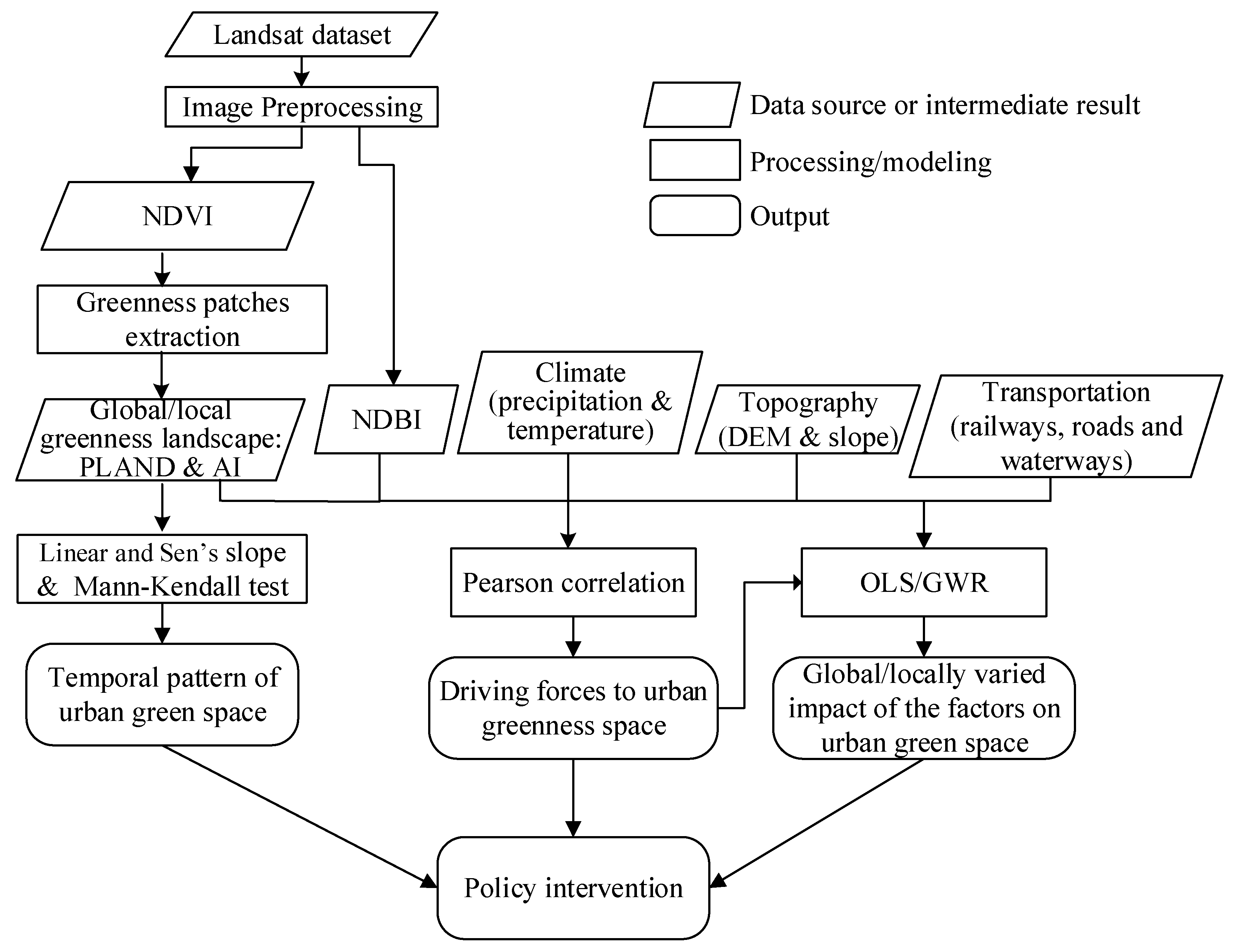
2. Study Area, Data Sources, and Methodology

2.1. Study Area

The study was performed for Wuhan metropolis, Hubei province, covering nearly 10,000 km2 in central China, as shown in Figure 1. Wuhan, as the capital city of Hubei province, is a megacity in central China. It is one of the 17 cities included in the global sustainable development plan issued by the United Nations Development Programme and the United Nations Environment Programme [39]. Located at the intersection of the Yangtze River and Han River, the metropolis is spatially divided into three districts by the rivers, including Hankou, Wuchang, and Hanyang. Famous for its hundreds of water bodies (lakes) and rivers, it is well-known as a “river city”. The city is also characterized by uneven topography (ranging between 13 and 262 m above sea level), complicated water network, dense population (over 10 million), and intensified human-related activities. The area is covered by various land cover and land use types. Urbanized or built-up areas dominate mainly around the central part of the region. Croplands, forests, and grasslands spread mainly over the peri-urban or rural areas. Continuous urban expansion has transformed vegetation into built-up areas, causing significant shrinkage in the urban greenness space and imposing negative impacts on the urban ecosystem [40]. Therefore, understanding the changes of urban greenness space and the driving factors of the changes have been urgently needed to promote a sustainable urban ecosystem for Wuhan metropolis.

2.2. Data Sources

The data sources used in the study can be grouped into 4 categories—human-related socio-economic activities, climate, topography, and urban greenness indicators—with the first three serving as explanatory variables and the last as target or dependent variables, as shown in Table 1. The details of the datasets are described below.
Google Earth Engine (GEE) is a planetary-scale platform for earth science data and analysis, useful for researchers to detect changes of the earth’s surface [41]. The latest updated transportation dataset of road network and railways in 2018 was obtained from the transportation bureau of the local government. Furthermore, rivers and waterways were classified from Landsat images on the GEE platform. Those variables are closely related to the local economy and thus are related to urban land changes.
Climate conditions can alter urban greenness landscapes. Precipitation and temperature are two key variables, as they may affect the urban greenness based on a previous study [42]. Precipitation and temperature at a monthly scale composed of more than 650 climatic stations were obtained from the China Meteorological Data Sharing Platform during the years 2000–2018 (http://cdc.cma.gov.cn) and spatially interpolated using thin-plate smoothing splines [43]. Annually accumulated precipitation and mean temperature were then clipped by the study boundary.
A digital elevation model (DEM) was used to represent elevation. DEM data, which are Global Multi-resolution Terrain Elevation Data 2010 with a spatial resolution of about 30 m, were acquired from GEE. The topographic slope was derived from DEM on GEE [44]. The terrain characteristics may affect vegetation cover and thus should be examined in terms of their impact on urban vegetation cover.
The normalized difference vegetation index (NDVI) is often used as a proxy for vegetation coverage [45]. It is computed through the two reflectance bands, near infrared (NIR) and red (R), from remote sensing imagery in the form of
N D V I = ( N I R R ) / ( N I R + R ) .
GEE provides online access to archived Landsat data, which includes Landsat 5 Thematic Mapper (TM) from 1984 to 2012, Landsat 7 Enhanced Thematic Mapper Plus (ETM+) from 1999 to present, and Landsat 8 Operational Land Imager (OLI) and Thermal Infrared Sensor (TIRS) from 2013 to present [41,46,47]. ETM+ suffered from the failure of the scan line corrector (SLC) starting from May 2003, which resulted in data gaps in the acquired images. Image preprocessing included gap filling for ETM+ SLC-off images and cloud filtering. A simple and effective method for filling gaps in ETM+ SLC-off images using the neighborhood similar pixel interpolator (NSPI), which works especially well in heterogeneous regions as detailed by Chen et al. [48] and Asare et al. [49], was applied to improve ETM+ image quality. To minimize the effects of clouds and cloud shadows from the images, a cloud score algorithm based on a combination of brightness, temperature, and the normalized difference snow index was applied to compute a cloud-likelihood score based on GEE’s built-in algorithm (i.e., ee.Algorithms.Landsat.simpleCloudScore) and pixels with the score greater than 10 were excluded [50,51]. The preprocessed Landsat imagery series enabled the computation of long-term NDVI series for the study region. An annual maximum composite NDVI for each year during 2000–2018 was derived from the computed NDVI time-series.
The normalized difference built-up index (NDBI) is an index representing the cover of the impervious surface of a city and is an indicator of human activities in urban areas [52]. NDBI is strongly correlated to the impervious surface of the city [53]. To compute NDBI, the reflectance of the two bands of the middle infrared (MIR) and near infrared band are taken, in the form of [53,54]
N D B I = ( M I R N I R ) / ( M I R + N I R ) .
A composite of maximum NDBI was derived for each year during 2000–2018 based on the multiple time-series maps of NDBI with that year.

2.3. Methods

The overall framework for the analysis of the dynamics and the driving factors of the urban greenness space is shown in Figure 2.
First, urban greenness patches were extracted based on image classification using GEE [40]. An urban greenness patch was defined as a continuous vegetated area covered by either grassland, forestry, croplands, or any combination of the above. Two urban greenness landscape indices, namely percentage of landscape (PLAND hereafter) and aggregation index (AI hereafter) were computed to build a time-series dataset. PLAND measures the area of the land cover type standardized by the total area of the landscape [34], while AI reflects the degree of aggregation or extension of patches for that type [55]. PLAND is an indicator used to measure the proportion of urban greenness landscapes compared to a region of interest. The abundance of greenness space is indicated by PLAND. The temporal changes, either an increase or decrease, in the area of greenness space can be illustrated by inter-annual dynamics of PLAND. For a given region R, PLAND is computed as
PLAND = i = 1 n a i / A R * 100 %
where AR is the total area of R, ai is the area of the greenness patch i (i = 1, 2, …, n, where n is the total number of urban greenness patches).
The aggregation index (AI) indicates the clustering pattern of urban greenness cover, which is a useful measurement for vegetation fragmentation. For the urban greenness landscape, AI is defined as the ratio of the edges shared by greenness pixels to the total number of edges, in the form of
A I g r e e n = g g r e e n g r e e n / m a x g r e e n
where ggreen-green is the number of all shared edges between pixels of greenness patches, maxgreen is the maximum number of edges between pixels of greenness patches. The highest level of clustering indicates greenness pixels sharing the most possible edges (AI will be close to 1), while the lowest level of aggregation means greenness pixels sharing no edges (AI = 0, greenness pixels completely disaggregated) [37]. To examine the temporal dynamics of the urban greenness space, Sen’s slope and the Mann–Kendall trend test were performed on the time-series of the NDVI and the landscape indices. To account for the possible driving forces, Pearson correlation analysis was applied to quantify the correlation between the landscape indices and the explanatory variables. Then two regression models, namely, ordinary least square (OLS) and the geographically weighted regression (GWR) model, were performed to reveal the global and locally varied relationships between the explanatory variables and the target landscape indices. The coefficients between the explanatory variables and the indices of urban greenness landscape from GWR were mapped so that the location-dependent impact from the driving forces could visualized.
PLAND and AI can be processed globally and locally. When the entire region is selected, a global version of PLAND or AI will be defined. Conversely, a local version of the indices is processed for a predefined neighborhood. In the current study, a circular moving window with a radius of 200 pixels was defined to compute a local PLAND and AI, which is a local version capable of highlighting the spatially varied features of the indices.
The urban vegetation (through NDVI) and the urban greenness landscape (PLAND and AI) showed changes over the years. To explore the dynamics along the years, a linear regression analysis and Sen’s slope were applied [56]. For a set of pairs (i, xi) or (j, xj), where xi (or xj) is a time-series and i (or j) is the sequential position of the element in the dataset, Sen’s slope β is calculated as
β = Median { ( x j x i ) / ( j i ) : i < j } .
A positive β suggests that the time-series show a rising trend, and vice versa. The significance of trend in the greenness landscape indices (PLAND and AI) and vegetation greenness level (NDVI) was evaluated using the Mann–Kendall test. The Kendall τ (−1 to +1) obtained from the Mann–Kendall statistics could be used to measure the significance of the trend [57]. Thus, the dynamics of NDVI, PLAND, and AI during 2000–2018 were tested using Sen’s slope and Mann–Kendall trend analysis.
The spatial distribution patterns of the urban greenness landscape could be attributed to various factors. To examine the factors that may have impacted on the landscape patterns, three steps were taken to investigate the relationship between the temporally averaged results of the explanatory and target variables. First, Pearson correlation analysis, which takes two variables X and Y as input, computes correlation coefficient (P) or the ratio of the covariance between the variables (Cov(X,Y)) to their standard deviation products [58], using the formula
P X , Y = C o v ( X , Y ) / σ X · σ Y .
The computed coefficient ranges between −1 to 1 and a value close to 0 indicates the least correlation between the variables [59]. By computing the correlation coefficients between the input factors and the target landscape indices, those explanatory factors that show significantly correlated to PLAND and AI could be retained for further analysis.
Ordinary least squares (OLS) regression is a global statistical method that estimates the relationship between independent variables and a dependent variable. With the input of the explanatory variables and the landscape indices, OLS can output the coefficients that indicate the direction and magnitude of the impact from the independent variables. Nevertheless, due to non-stationary or heterogeneous characteristics of most spatial patterns, a widely applied local regression model, namely, geographically weighted regression (GWR), has been applied in many applications to capture spatially varied relationships between multiple variables [60]. Compared to the global regression model such as OLS, GWR models the local relationships between predictors and a dependent variable, in the form of
y i = β 0 ( u i , v i ) + k = 1 n β k ( u i , v i ) x i k + ε i , i = 1 , 2 , ... , n
where yi is the dependent variable at location i, xik (k = 1, 2, …, n, and n is the number of explanatory variables) is the independent variable, (ui, vi) is the coordinate of the location i, β0(ui, vi) is the intercept of a constant for spatial variability, βk(ui, vi) is the estimated coefficient for the kth explanatory variable, and εi is the random error. The kernel and bandwidth are key parameters in the GWR model that affect model accuracy. Gaussian kernel was decided in the current work. The optimal bandwidth was determined on estimated distance from spatial autocorrelation of the dependent variables (PLAND and AI). Explanatory variables input into OLS and the local model need to be free of multicollinearity [61]. To avoid multicollinearity among the variables, variance inflation factor (VIF) can be checked, where VIF values greater than 10 indicate multicollinearity [62]. The adjusted coefficient of determination (RAdj.2) and corrected Akaike information criterion (AICc) serve as a measure of goodness of fit to determine whether a global or local model should be applied to have a better interpretation for the patterns in the analyzed data [60].

3. Results

3.1. Temporal Dynamics of Urban Greenness

A time-series analysis using bivariate linear regression and Sen’s slope against the years, as well as the Mann–Kendall trend test on the urban greenness landscape indices, i.e., PLAND and AI, revealed that not only the total area of urban greenness space showed a decrease, but also the urban greenness patches tended to be more fragmented, as both PLAND and AI presented significant decline over the years. Table 2 shows the results from the trend analysis by bivariate linear regression and Sen’s slope.
Both the linear slope and Sen’s slope indicated a significantly negative value for PLAND and AI (p < 0.01, n = 19). The result revealed that more vegetated area was converted to non-vegetated land cover, most likely due to rapid urban expansion. At the same time, larger vegetated patches were found to be split into smaller ones, most likely due to intensified human activities. Nevertheless, the result demonstrated that the averaged NDVI still showed an overall increasing trend over the years, meaning the health of urban vegetation was improving at least for some areas that were not converted into built-up areas. Figure 3 shows two typical NDVI maps for the starting year (2000, Figure 3a) and the end (the year 2018, Figure 3b). The urbanized area expanded outside significantly from the urban center, explaining the reduction of the urban greenness space in the region. However, the overall greenness in terms of NDVI showed improvement in the year 2018 if compared to that in 2000. Though the detailed explanation remains undiscovered, the improvement of NDVI over vegetated areas might be attributed to recent reforestation programs in the city [63] and/or global warming [64].

3.2. Factor Analysis for the Dynamics of the Urban Greenness

The preliminary analysis selected a set of candidate factors, including the climatic variables (precipitation and surface temperature), terrain (DEM and slope), transportation impact (density of railways, roads, and waterways), and urbanization level (in the proxy of the normalized difference built-up index or NDBI). Those factors have proved to be related to the changes of the urban greenness landscape by many other studies [3,20]. The combination of those economic and environmental factors may provide a more comprehensive view for understanding the driving forces for the urban greenness space. First, Pearson correlation analysis was conducted to examine if there exists a strong bivariate correlation between any of the candidate variables and the urban greenness landscape indices. The correlation coefficients between the candidate variables and the indices (PLAND and AI) are shown in Table 3. Except for the temperature, all the other variables presented a significant correlation to the two urban greenness landscape indices. The significant and positive coefficients from the variables DEM, slope, and precipitation suggest strong positive effect to the improvement of the urban greenness landscape indices, while the negative values from the NDBI and transportation pathways (waterways, roads, and railways) indicated that they reduced the landscape indices.
While the coefficients from the correlation analysis revealed the relationship between each individual variable and the indicators of the urban greenness landscape (i.e., PLAND and AI), multivariate analysis with input from the combination of the factors could be a better overview, as the selected individual variables may have multicollinearity in terms of the explanation effect to the dependent variables. Thus, the multicollinearity for the selected factors that are significantly correlated to the greenness landscape indices was further tested. Results indicated that the waterways and railway presented a serious multicollinearity (VIF > 8), as shown in Table 4. Transportation accessibility is usually regarded as a critical factor that may alter vegetation cover [23]. Out of the three selected transportation elements, the distance to waterways and the density of railways presented strong correlation with the road density. The multicollinearity suggests that the variable road alone could provide sufficient explanation power to the patterns of urban greenness space and that the waterways and railway could be replaced by the road network in the multivariate analysis. Therefore, the variables of waterway and railway were eliminated from further analysis.

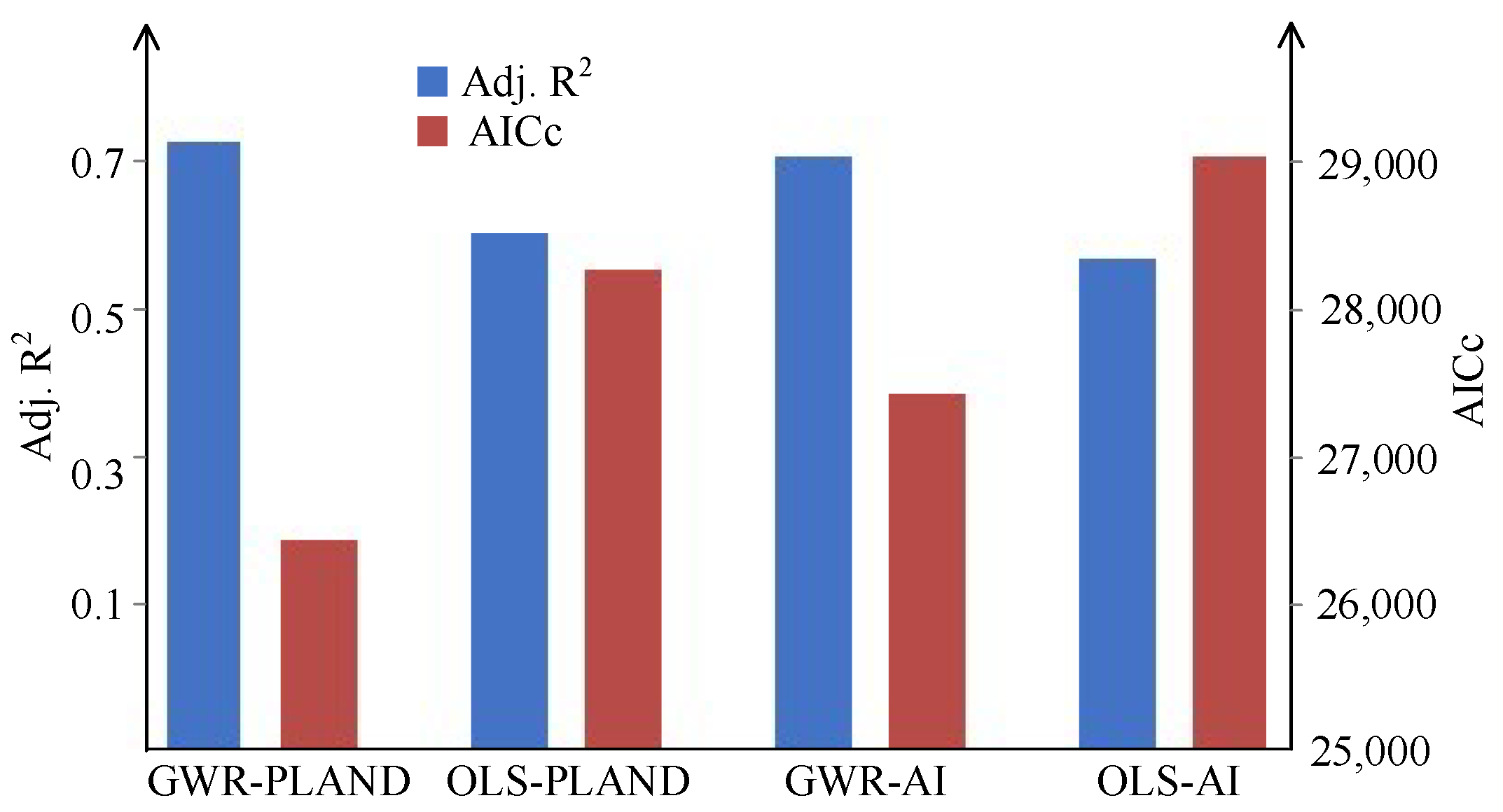
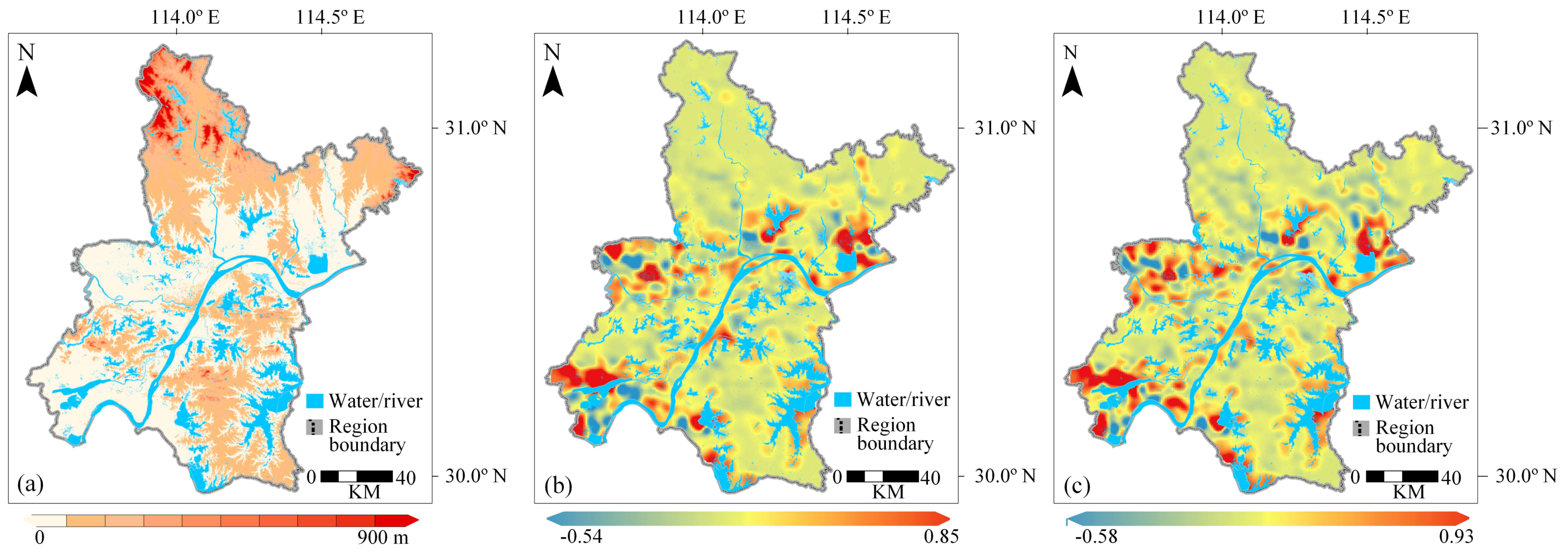
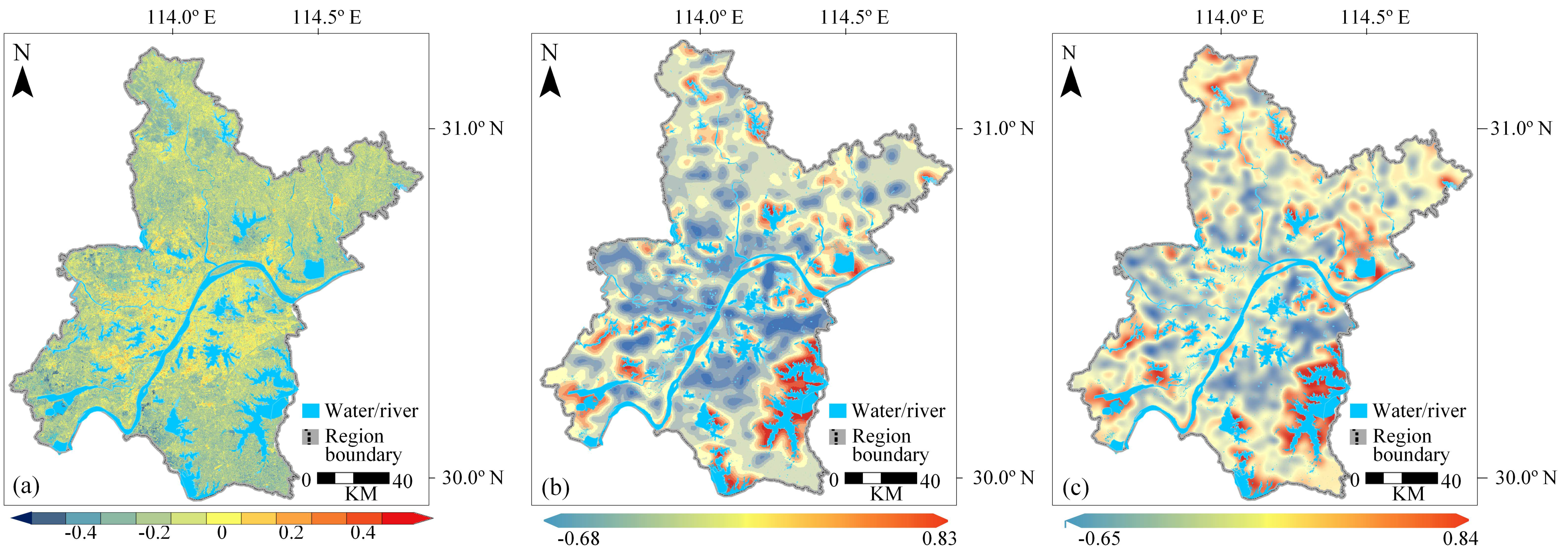
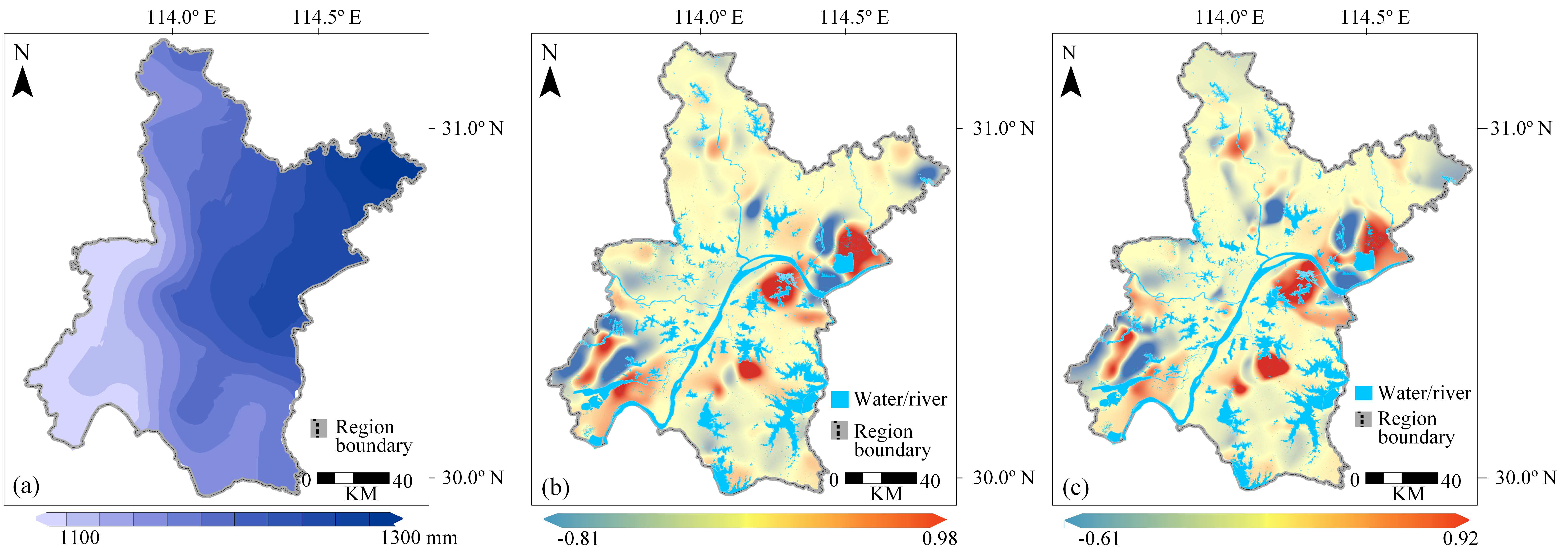
3.3. Analysis of Driving Factors on Urban Greenness Landscape Based on GWR

The variables, namely, DEM, slope, NDVI, road, and precipitation, were selected based on the result from the correlation and multicollinearity analysis. Ordinary least squares (OLS) regression and GWR analysis were performed on the landscape indices PLAND and AI, respectively. Figure 4 shows that a moderate model performance was obtained from the OLS regression (adjusted R2 = 0.604 and 0.593 for PLAND and AI, respectively), indicating a good fit of the OLS model [65], which further confirms the explanation power of the selected variables to the dependent variables. While OLS creates global estimates for the entire region, the GWR generates a set of spatially varying estimates defined by a local model. Thus, GWR differentiates location-dependent impact on the target indices from the variables. The result indicates that the GWR model produced a higher adjusted R2 for both PLAND and AI indices, suggesting GWR is more reliable than OLS. Furthermore, the AICc from the GWR model was smaller than that from the OLS model for both PLAND and AI. Thus, applying the GWR model is more preferable in terms of the explanation power of the impact on the urban greenness landscape indices from the selected variables.
The elevation variable DEM presented either positive or negative impact on the landscape indices. The elevation and the regression coefficients with PLAND and AI are presented in Figure 5. The high elevated areas in the northern part did not show much impact on the two indices. The central part and southwestern areas imposed positive impact on both PLAND and AI, as revealed by the high positive coefficients, suggesting that areas at lower elevation tended to maintain good urban vegetation coverage (higher PLAND) and keep vegetation clustered (higher AI). However, the negative impact from elevation is more complicated. For example, the relatively high elevated area in the southern part showed a negative coefficient. It is noteworthy that the impact of elevation on PLAND and AI showed an identical pattern in terms of the spatial distribution of each coefficient, which suggests that elevation may impose similar impacts on both the abundance and fragmentation of urban greenness space in the current study area.
The slope variable, as well as its impact on the two landscape indices are presented in Figure 6. As the slope was derived from the elevation (DEM), the northern part, which was dominated by mountains, showed steep slopes. The coefficients of its impact on the landscape indices presented similar patterns to those from the DEM. A few clustered places in the central and southwestern parts of the region showed positive impact to PLAND and AI. The areas with steep slope (e.g., the northern part) did not present an obvious impact on the two indices. Those locations that showed significant negative coefficients should be given special attention as those areas tended to suffer substantial loss in urban greenness space or to fragment.
The urbanization process partially reflects the impact of human activities on urban ecosystems. The study area has experienced significant urban expansion, or increased built-up area, during the years. The urbanization of the city expanded from the center of the area and higher NDBI values were mainly distributed around the central part, as indicated in Figure 7a. The regression coefficients of the NDBI with PLAND and AI, as shown in Figure 7b,c, illustrated that the values were negative around the region of the central part and that urbanization in the greater part of the central area was likely to reduce urban greenness coverage and induce vegetation cover fragmentation. The areas that showed positive correlations between NDBI and the urban greenness indices mainly located close to water bodies. In fact, while considerable water bodies were found to be converted into urbanized land in the past two decades, it is not uncommon to see mosaicked vegetation in the newly built-up areas in the study area [66]. Thus, urban greenness space showed improvement around neighborhoods of water bodies.
Precipitation proves to be a significant factor to vegetation cover. The annually accumulated precipitation ranged between 1100 and 1300 mm, with an increasing trend from northeast to southwest, as shown in Figure 8a. Many studies have revealed a positive contribution of precipitation to vegetation growth in urban ecosystems [67]. We found that the impact of the precipitation on the urban greenness landscape was heterogeneously distributed with significant spatial variations. The negative and positive impact from precipitation on the landscape indices was found to present a clustering pattern, as shown in Figure 8b,c, suggesting the complicated impact on the urban greenness distribution from the precipitation variable. The variation in the impact from precipitation was likely related to the hundreds of water bodies (rivers and lakes) in the study area, making the effect of precipitation on PLAND and AI spatially varied. The distribution of water bodies may affect the environment of the nearby areas and thus the impact from precipitation did not present a uniform pattern over the whole study region.
The road network serves as another proxy for human activities which imposed spatially varied impact on urban greenness. Road network density was highest around the central region, as shown in Figure 9a, where the road density showed either negative or no obvious impact on the greenness indices, as shown in Figure 9b,c, meaning a highly densified transportation network tends to decrease urban vegetation space and fragment urban greenness patches. In contrast, the road network showed a strong positive effect on the landscape indices in some parts of the peri-urban areas, which means that the greenness space there could be improved with the building of a limited density transportation network. It is of policy implication to note that the road network might impose the opposite impact on the urban vegetation space, depending on the current road network density.

4. Discussions

Urban vegetation plays vital role for the sustainable development of urban ecosystems. With rapid urbanization and increasing intensified human-related activities in many cities, decreased ecological services have been observed due to significant loss of urban greenness [13,68]. Many studies have confirmed that urbanization imposed a direct impact on urban greenness space [10], and reduced exposure to greenness could cause environmental stresses to public health issues [1]. Because the world population continues to rise while cities provide more advantageous conditions, a significant amount of people in rural areas tend to live in urban areas to enjoy a convenient life [38]; thus, the increased population plays as a strong potential driver for urbanization, which may occupy urban greenness space.
The urban greenness landscape indices, i.e., PLAND and AI, prove to be useful in revealing the urban vegetation coverage and fragmentation/clustering patterns in distribution. Through spatial analysis, it is meaningful to know the changing trend in the landscape indices, as urban greenness space is closely related to public health of urban residents [7,58]. Moreover, investigating the underlying factors that are contributing to the changes would be even more important for urban land planning. Previous studies indicated that the influential factors of urban greenness were multiple and that misleading results might be drawn without a systematic analysis on its driving forces [17,42]. Those factors are composed of not only natural environments but also human-related activities [69]. Those influencing factors could impose a complex impact on the target urban greenness landscape [70].
The urban greenness changes and the possible driving factors for the changes can be explored through ordinary least square (OLS) regression and geographically weighted regression (GWR). Remotely sensed imagery, namely, the Landsat series, provides a valuable dataset to map the dynamics of the urban greenness space. There are a number of indices that could be applied to quantify urban greenness space. This study measures urban greenness patterns by two landscape indices, i.e., PLAND and AI. Since PLAND captures the proportion of urban greenness cover out of the total land area and AI measures the aggregation of greenness patches, the combination of the two could reflect the overall patterns of the urban greenness space. The time-series analysis of Sen’s slope and Mann–Kendall trend testing showed usefulness in revealing the dynamics of the indices over the years. The results showed that the coverage of the urban greenness space had significantly decreased, which is in accordance with our previous study [19]. Moreover, the study also found that the urban greenness was increasingly fragmented over the years.
The identified driving forces of the landscape indices, as revealed from the OLS and GWR analysis, suggest that both the natural/environmental factors (including elevation, topographic slope, and precipitation) and human-related activities (e.g., urbanization intensity via NDBI and the road network) showed significant impact on urban greenness space in Wuhan city. Overall, the landscape indices were positively correlated with the natural factors but negatively correlated with the human-related activities. Because the natural and social factors demonstrated high variation across the region, GWR was applied to map the spatially varied impact, revealing the influential directions (either positive or negative) and magnitude from each of the factors. Those spatially varied patterns were illustrated in the coefficients of the factors against the target PLAND and AI. Urban planning policies targeting better urban ecosystem services should give more attention to urbanization control and location-dependent construction of the transportation networks and sensitive areas with urban greenness space that could be significantly affected by terrain characteristics and climatic factors. The identified driving factors and their spatially varied impact on the urban greenness indices can provide useful information to design policies targeting sustainable development of urban ecosystems.

5. Conclusions

This study has selected Wuhan, China as the case area to examine the temporal changes of urban greenness space and the driving factors explaining the patterns in the changes. The combination of the landscape indices, PLAND and AI, is useful to reveal both the abundance and clustering pattern of urban greenness space. It was found that the coverage of the urban greenness space had significantly decreased, and the urban greenness patches were more fragmented. Human and natural factors imposed considerable impact on urban greenness space. Road network density, normalized difference built-up index (NDBI), terrain elevation and slope, and precipitation were significantly correlated to the landscape indices. The study verified that GWR is more reliable than OLS in studying the relationship between the spatial variables. Applying the GWR model is more preferable in terms of the explanation power of the impact on the urban greenness landscape indices from the selected variables. GWR modeling also captures the spatially varied impact from the factors, which is more desirable for making location-specific urban planning.
The current work did not differentiate the vegetation cover types, for example, farmland crops or other plant types such as trees, shrubs, and grasses. The changes in those vegetation cover types could be induced from human activities (cultivation) or natural process (succession) and thus involves different mechanisms for the changes in greenness space. Future work may pay attention to the impact on different vegetation types (forestry, grassland, and croplands) from the driving factors.

Author Contributions

Conceptualization, Z.S. and R.L.; methodology, Z.S.; software, C.Y.; validation, C.Y. and R.L.; formal analysis and investigation, Z.S.; resources and data curation, R.L.; writing—original draft preparation and visualization, C.Y.; writing—review and editing, Z.S. and R.L. All authors have read and agreed to the published version of the manuscript.

Funding

This research was funded by the National Natural Science Foundation of China grant number 41871296.

Conflicts of Interest

The authors declare no conflict of interest.

References

  1. Crouse, D.L.; Pinault, L.; Balram, A.; Hystad, P.; Peters, P.A.; Chen, H.; van Donkelaar, A.; Martin, R.V.; Ménard, R.; Robichaud, A.; et al. Urban greenness and mortality in Canada’s largest cities: A national cohort study. Lancet Planet. Health 2017, 1, e289–e297. [Google Scholar] [CrossRef]
  2. United Nations, Department of Economic and Social Affairs, Population Division. World Urbanization Prospects: The 2018 Revision (ST/ESA/SER.A/420); United Nations: New York, NY, USA, 2019. [Google Scholar]
  3. Yang, G.; Zhao, Y.; Xing, H.; Fu, Y.; Liu, G.; Kang, X.; Mai, X. Understanding the changes in spatial fairness of urban greenery using time-series remote sensing images: A case study of Guangdong-Hong Kong-Macao Greater Bay. Sci. Total Environ. 2020, 715, 136763. [Google Scholar] [CrossRef] [PubMed]
  4. Follmann, A.; Hartmann, G.; Dannenberg, P. Multi-temporal transect analysis of peri-urban developments in Faridabad, India. J. Maps 2018, 14, 17–25. [Google Scholar] [CrossRef]
  5. Tian, G.; Qiao, Z. Assessing the impact of the urbanization process on net primary productivity in China in 1989–2000. Environ. Pollut. 2014, 184, 320–326. [Google Scholar] [CrossRef] [PubMed]
  6. Buyantuyev, A.; Wu, J. Urbanization diversifies land surface phenology in arid environments: Interactions among vegetation, climatic variation, and land use pattern in the Phoenix metropolitan region, USA. Landsc. Urban Plan. 2012, 105, 149–159. [Google Scholar] [CrossRef]
  7. Huang, C.; Yang, J.; Lu, H.; Huang, H.; Yu, L. Green Spaces as an Indicator of Urban Health: Evaluating Its Changes in 28 Mega-Cities. Remote Sens. 2017, 9, 1266. [Google Scholar] [CrossRef] [Green Version]
  8. Cârlan, I.; Mihai, B.A.; Nistor, C.; Große-Stoltenberg, A. Identifying urban vegetation stress factors based on open access remote sensing imagery and field observations. Ecol. Inform. 2020, 55, 101032. [Google Scholar] [CrossRef]
  9. Liu, Y.; Wang, R.; Grekousis, G.; Liu, Y.; Yuan, Y.; Li, Z. Neighbourhood greenness and mental wellbeing in Guangzhou, China: What are the pathways? Landsc. Urban Plan. 2019, 190, 103602. [Google Scholar] [CrossRef]
  10. Dennis, M.; Barlow, D.; Cavan, G.; Cook, P.; Gilchrist, A.; Handley, J.; James, P.; Thompson, J.; Tzoulas, K.; Wheater, C.P.; et al. Mapping Urban Green Infrastructure: A Novel Landscape-Based Approach to Incorporating Land Use and Land Cover in the Mapping of Human-Dominated Systems. Land 2018, 7, 17. [Google Scholar] [CrossRef] [Green Version]
  11. Wu, W.; Wang, M.; Zhu, N.; Zhang, W.; Sun, H. Residential satisfaction about urban greenness: Heterogeneous effects across social and spatial gradients. Urban For. Urban Green. 2019, 38, 133–144. [Google Scholar] [CrossRef]
  12. Sulander, T.; Karvinen, E.; Holopainen, M. Urban Green Space Visits and Mortality Among Older Adults. Epidemiology 2016, 27, e34–e35. [Google Scholar] [CrossRef] [PubMed]
  13. Hussein, S.O. Monitoring urban greenness evolution using multitemporal Landsat imagery in the city of Erbil (Iraq). Cent. Eur. Geol. 2019, 62, 15–26. [Google Scholar] [CrossRef]
  14. Zhong, Q.; Ma, J.; Zhao, B.; Wang, X.; Zong, J.; Xiao, X. Assessing spatial-temporal dynamics of urban expansion, vegetation greenness and photosynthesis in megacity Shanghai, China during 2000–2016. Remote Sens. Environ. 2019, 233, 111374. [Google Scholar] [CrossRef]
  15. Lu, L.; Weng, Q.; Guo, H.; Feng, S.; Li, Q. Assessment of urban environmental change using multi-source remote sensing time series (2000–2016): A comparative analysis in selected megacities in Eurasia. Sci. Total Environ. 2019, 684, 567–577. [Google Scholar] [CrossRef] [PubMed]
  16. Chen, B.; Nie, Z.; Chen, Z.; Xu, B. Quantitative estimation of 21st-century urban greenspace changes in Chinese populous cities. Sci. Total Environ. 2017, 609, 956–965. [Google Scholar] [CrossRef] [PubMed]
  17. Franco, S.F.; Macdonald, J.L. Measurement and valuation of urban greenness: Remote sensing and hedonic applications to Lisbon, Portugal. Reg. Sci. Urban Econ. 2018, 72, 156–180. [Google Scholar] [CrossRef]
  18. Drummond, M.A.; Stier, M.P.; Diffendorfer, J.; Jay, E. Historical land use and land cover for assessing the northern Colorado Front Range urban landscape. J. Maps 2019, 15, 89–93. [Google Scholar] [CrossRef]
  19. Sha, Z.; Ali, Y.; Wang, Y.; Chen, J.; Tan, X.; Li, R. Mapping the changes in urban greenness based on localized spatial association analysis under temporal context using MODIS data. ISPRS Int. J. Geo-Inform. 2018, 7, 407. [Google Scholar] [CrossRef] [Green Version]
  20. Miller, D.L.; Alonzo, M.; Roberts, D.A.; Tague, C.L.; McFadden, J.P. Drought response of urban trees and turfgrass using airborne imaging spectroscopy. Remote Sens. Environ. 2020, 240, 111646. [Google Scholar] [CrossRef]
  21. El Garouani, A.; Mulla, D.J.; El Garouani, S.; Knight, J. Analysis of urban growth and sprawl from remote sensing data: Case of Fez, Morocco. Int. J. Sustain. Built Environ. 2017, 6, 160–169. [Google Scholar] [CrossRef]
  22. Rimal, B.; Zhang, L.; Stork, N.; Sloan, S.; Rijal, S. Urban expansion occurred at the expense of agricultural lands in the Tarai region of Nepal from 1989 to 2016. Sustainability 2018, 10, 1341. [Google Scholar] [CrossRef] [Green Version]
  23. Fan, C.; Johnston, M.; Darling, L.; Scott, L.; Liao, F.H. Land use and socio-economic determinants of urban forest structure and diversity. Landsc. Urban Plan. 2019, 181, 10–21. [Google Scholar] [CrossRef]
  24. Güneralp, B.; Seto, K.C.; Ramachandran, M. Evidence of urban land teleconnections and impacts on hinterlands. Curr. Opin. Environ. Sustain. 2013, 5, 445–451. [Google Scholar] [CrossRef]
  25. Rimal, B.; Zhang, L.; Keshtkar, H.; Sun, X.; Rijal, S. Quantifying the spatiotemporal pattern of urban expansion and hazard and risk area identification in the Kaski District of Nepal. Land 2018, 7, 37. [Google Scholar] [CrossRef] [Green Version]
  26. Cui, Y.; Cheng, D.; Choi, C.E.; Jin, W.; Lei, Y.; Kargel, J.S. The cost of rapid and haphazard urbanization: Lessons learned from the Freetown landslide disaster. Landslides 2019, 1167–1176. [Google Scholar] [CrossRef] [Green Version]
  27. Wang, J.; Zhou, W.; Qian, Y.; Li, W.; Han, L. Quantifying and characterizing the dynamics of urban greenspace at the patch level: A new approach using object-based image analysis. Remote Sens. Environ. 2018, 204, 94–108. [Google Scholar] [CrossRef]
  28. Xie, Y.; Sha, Z.; Yu, M. Remote sensing imagery in vegetation mapping: A review. J. Plant Ecol. 2008, 1, 9–23. [Google Scholar] [CrossRef]
  29. Zhu, Z.; Fu, Y.; Woodcock, C.E.; Olofsson, P.; Vogelmann, J.E.; Holden, C.; Wang, M.; Dai, S.; Yu, Y. Including land cover change in analysis of greenness trends using all available Landsat 5, 7, and 8 images: A case study from Guangzhou, China (2000–2014). Remote Sens. Environ. 2016, 185, 243–257. [Google Scholar] [CrossRef] [Green Version]
  30. Kabisch, N.; Selsam, P.; Kirsten, T.; Lausch, A.; Bumberger, J. A multi-sensor and multi-temporal remote sensing approach to detect land cover change dynamics in heterogeneous urban landscapes. Ecol. Indic. 2019, 99, 273–282. [Google Scholar] [CrossRef]
  31. Dou, Y.; Kuang, W. A comparative analysis of urban impervious surface and green space and their dynamics among 318 different size cities in China in the past 25 years. Sci. Total Environ. 2020, 706, 135828. [Google Scholar] [CrossRef]
  32. Wang, W.; Lin, Z.; Zhang, L.; Yu, T.; Ciren, P.; Zhu, Y. Building visual green index: A measure of visual green spaces for urban building. Urban For. Urban Green. 2019, 40, 335–343. [Google Scholar] [CrossRef]
  33. Threlfall, C.G.; Ossola, A.; Hahs, A.K.; Williams, N.S.G.; Wilson, L.; Livesley, S.J. Variation in Vegetation Structure and Composition across Urban Green Space Types. Front. Ecol. Evol. 2016, 4, 66. [Google Scholar] [CrossRef] [Green Version]
  34. Harms, T.M.; Murphy, K.T.; Lyu, X.; Patterson, S.S.; Kinkead, K.E.; Dinsmore, S.J.; Frese, P.W. Using landscape habitat associations to prioritize areas of conservation action for terrestrial birds. PLoS ONE 2017, 12, e0173041. [Google Scholar] [CrossRef] [PubMed]
  35. Hamad, R.; Kolo, K.; Balzter, H. Post-War Land Cover Changes and Fragmentation in Halgurd Sakran National Park (HSNP), Kurdistan Region of Iraq. Land 2018, 7, 38. [Google Scholar] [CrossRef] [Green Version]
  36. Kowe, P.; Mutanga, O.; Odindi, J.; Dube, T. A quantitative framework for analysing long term spatial clustering and vegetation fragmentation in an urban landscape using multi-temporal landsat data. Int. J. Appl. Earth Obs. Geoinf. 2020, 88, 102057. [Google Scholar] [CrossRef]
  37. He, H.S.; DeZonia, B.E.; Mladenoff, D.J. An aggregation index (AI) to quantify spatial patterns of landscapes. Landsc. Ecol. 2000, 15, 591–601. [Google Scholar] [CrossRef]
  38. Wang, Y.; Sha, Z.; Tan, X.; Lan, H.; Liu, X.; Rao, J. Modeling urban growth by coupling localized spatio-temporal association analysis and binary logistic regression. Comput. Environ. Urban Syst. 2020, 81, 101482. [Google Scholar] [CrossRef]
  39. He, Q.; Tan, R.; Gao, Y.; Zhang, M.; Xie, P.; Liu, Y. Modeling urban growth boundary based on the evaluation of the extension potential: A case study of Wuhan city in China. Habitat Int. 2018, 72, 57–65. [Google Scholar] [CrossRef]
  40. Khan, Y.A.; Wang, Y.; Sha, Z. Land Cover Change Analysis in Wuhan, China Using Google Earth Engine Platform and Ancillary Knowledge. In Communications in Computer and Information Science; Springer: Berlin, Germany, 2019; Volume 980, pp. 229–239. [Google Scholar]
  41. Gorelick, N.; Hancher, M.; Dixon, M.; Ilyushchenko, S.; Thau, D.; Moore, R. Google Earth Engine: Planetary-scale geospatial analysis for everyone. Remote Sens. Environ. 2017, 202, 18–27. [Google Scholar] [CrossRef]
  42. Lamchin, M.; Lee, W.K.; Jeon, S.W.; Wang, S.W.; Lim, C.H.; Song, C.; Sung, M. Long-term trend and correlation between vegetation greenness and climate variables in Asia based on satellite data. Sci. Total Environ. 2018, 618, 1089–1095. [Google Scholar] [CrossRef]
  43. Price, D.T.; McKenney, D.W.; Nalder, I.A.; Hutchinson, M.F.; Kesteven, J.L. A comparison of two statistical methods for spatial interpolation of Canadian monthly mean climate data. Agric. For. Meteorol. 2000, 101, 81–94. [Google Scholar] [CrossRef]
  44. Li, X.; Zhang, Y.; Jin, X.; He, Q.; Zhang, X. Comparison of digital elevation models and relevant derived attributes. J. Appl. Remote Sens. 2017, 11, 1. [Google Scholar] [CrossRef]
  45. Wang, Y.; Xue, Z.; Chen, J.; Chen, G. Spatio-temporal analysis of phenology in Yangtze River Delta based on MODIS NDVI time series from 2001 to 2015. Front. Earth Sci. 2019, 13, 92–110. [Google Scholar] [CrossRef]
  46. Patela, N.N.; Angiuli, E.; Gamba, P.; Gaughan, A.; Lisini, G.; Stevens, F.R.; Tatem, A.J.; Trianni, G. Multitemporal settlement and population mapping from landsatusing google earth engine. Int. J. Appl. Earth Obs. Geoinf. 2015, 35, 199–208. [Google Scholar] [CrossRef] [Green Version]
  47. Dong, J.; Xiao, X.; Menarguez, M.A.; Zhang, G.; Qin, Y.; Thau, D.; Biradar, C.; Moore, B. Mapping paddy rice planting area in northeastern Asia with Landsat 8 images, phenology-based algorithm and Google Earth Engine. Remote Sens. Environ. 2016, 185, 142–154. [Google Scholar] [CrossRef] [Green Version]
  48. Chen, J.; Zhu, X.; Vogelmann, J.E.; Gao, F.; Jin, S. A simple and effective method for filling gaps in Landsat ETM+ SLC-off images. Remote Sens. Environ. 2011, 115, 1053–1064. [Google Scholar] [CrossRef]
  49. Asare, Y.M.; Forkuo, E.K.; Forkuor, G.; Thiel, M. Evaluation of gap-filling methods for Landsat 7 ETM+ SLC-off image for LULC classification in a heterogeneous landscape of West Africa. Int. J. Remote Sens. 2020, 41, 2544–2564. [Google Scholar] [CrossRef]
  50. Huang, H.; Chen, Y.; Clinton, N.; Wang, J.; Wang, X.; Liu, C.; Gong, P.; Yang, J.; Bai, Y.; Zheng, Y.; et al. Mapping major land cover dynamics in Beijing using all Landsat images in Google Earth Engine. Remote Sens. Environ. 2017, 202, 166–176. [Google Scholar] [CrossRef]
  51. Zhang, D.D.; Zhang, L. Land cover change in the central region of the lower yangtze river based on landsat imagery and the google earth engine: A case study in Nanjing, China. Sensors 2020, 20, 2091. [Google Scholar] [CrossRef] [Green Version]
  52. Pan, X.; Zhu, X.; Yang, Y.; Cao, C.; Zhang, X.; Shan, L. Applicability of Downscaling Land Surface Temperature by Using Normalized Difference Sand Index. Sci. Rep. 2018, 8, 1–14. [Google Scholar] [CrossRef] [Green Version]
  53. Bhatti, S.S.; Tripathi, N.K. Built-up area extraction using Landsat 8 OLI imagery. GISci. Remote Sens. 2014, 51, 445–467. [Google Scholar] [CrossRef] [Green Version]
  54. Delgadillo Herrera, M.; Arreola Esquivel, M.M.; Toxqui-Quitl, C.; Padilla-Vivanco, A. Normalized difference indices in Landsat 5 TM satellite data. In Proceedings of the Current Developments in Lens Design and Optical Engineering XX; Johnson, R.B., Mahajan, V.N., Thibault, S., Eds.; SPIE: Bellingham, DC, USA, 2019; Volume 11104, p. 35. [Google Scholar]
  55. Wang, J.; Wang, K.; Zhang, M.; Zhang, C. Impacts of climate change and human activities on vegetation cover in hilly southern China. Ecol. Eng. 2015, 81, 451–461. [Google Scholar] [CrossRef]
  56. Han, J.C.; Huang, Y.; Zhang, H.; Wu, X. Characterization of elevation and land cover dependent trends of NDVI variations in the Hexi region, northwest China. J. Environ. Manag. 2019, 232, 1037–1048. [Google Scholar] [CrossRef]
  57. Gocic, M.; Trajkovic, S. Analysis of changes in meteorological variables using Mann-Kendall and Sen’s slope estimator statistical tests in Serbia. Glob. Planet. Chang. 2013, 100, 172–182. [Google Scholar] [CrossRef]
  58. Liu, B.; Bi, X.; Zhang, J.; Yuan, J.; Xiao, Z.; Dai, Q.; Feng, Y.; Zhang, Y. Insight into the critical factors determining the particle number concentrations during summer at a megacity in China. J. Environ. Sci. 2019, 75, 169–180. [Google Scholar] [CrossRef] [PubMed]
  59. Cong, N.; Shen, M.; Yang, W.; Yang, Z.; Zhang, G.; Piao, S. Varying responses of vegetation activity to climate changes on the Tibetan Plateau grassland. Int. J. Biometeorol. 2017, 61, 1433–1444. [Google Scholar] [CrossRef] [PubMed]
  60. Brunsdon, C.; Fotheringham, S.; Charlton, M. Geographically Weighted Regression. J. R. Stat. Soc. Ser. D Stat. 1998, 47, 431–443. [Google Scholar] [CrossRef]
  61. Özbay, N.; Toker, S. Multicollinearity in simultaneous equations system: Evaluation of estimation performance of two-parameter estimator. Comput. Appl. Math. 2018, 37, 5334–5357. [Google Scholar] [CrossRef]
  62. Tamura, R.; Kobayashi, K.; Takano, Y.; Miyashiro, R.; Nakata, K.; Matsui, T. Mixed integer quadratic optimization formulations for eliminating multicollinearity based on variance inflation factor. J. Glob. Optim. 2019, 73, 431–446. [Google Scholar] [CrossRef]
  63. Wang, Q.; Xiao, Q.; Liu, C.; Wang, K.; Ye, M.; Lei, A.; Song, X.; Kohata, K. Effect of reforestation on nitrogen and phosphorus dynamics in the catchment ecosystems of subtropical China: The example of the Hanjiang River basin. J. Sci. Food Agric. 2012, 92, 1119–1129. [Google Scholar] [CrossRef]
  64. Zhang, Y.; Feng, R.; Wu, R.; Zhong, P.; Tan, X.; Wu, K.; Ma, L. Global climate change: Impact of heat waves under different definitions on daily mortality in Wuhan, China. Glob. Health Res. Policy 2017, 2, 10. [Google Scholar] [CrossRef] [PubMed] [Green Version]
  65. Roy, D.P.; Kovalskyy, V.; Zhang, H.K.; Vermote, E.F.; Yan, L.; Kumar, S.S.; Egorov, A. Characterization of Landsat-7 to Landsat-8 reflective wavelength and normalized difference vegetation index continuity. Remote Sens. Environ. 2016, 185, 57–70. [Google Scholar] [CrossRef] [PubMed] [Green Version]
  66. Shi, L.; Ling, F.; Foody, G.M.; Chen, C.; Fang, S.; Li, X.; Zhang, Y.; Du, Y. Permanent disappearance and seasonal fluctuation of urban lake area in Wuhan, China monitored with long time series remotely sensed images from 1987 to 2016. Int. J. Remote Sens. 2019, 40, 8484–8505. [Google Scholar] [CrossRef]
  67. Paolini, L.; Schwendenmann, L.; Aráoz, E.; Powell, P.A. Decoupling of the urban vegetation productivity from climate. Urban For. Urban Green. 2019, 44, 126428. [Google Scholar] [CrossRef]
  68. Dong, Y.; Liu, H.; Zheng, T. Does the connectivity of urban public green space promote its use? An empirical study of Wuhan. Int. J. Environ. Res. Public Health 2020, 17, 297. [Google Scholar] [CrossRef] [PubMed] [Green Version]
  69. Reygadas, Y.; Jensen, J.L.R.; Moisen, G.G.; Currit, N.; Chow, E.T. Assessing the relationship between vegetation greenness and surface temperature through Granger causality and Impulse-Response coefficients: A case study in Mexico. Int. J. Remote Sens. 2020, 41, 3761–3783. [Google Scholar] [CrossRef]
  70. Wang, H.F.; Qureshi, S.; Qureshi, B.A.; Qiu, J.X.; Friedman, C.R.; Breuste, J.; Wang, X.K. A multivariate analysis integrating ecological, socioeconomic and physical characteristics to investigate urban forest cover and plant diversity in Beijing, China. Ecol. Indic. 2016, 60, 921–929. [Google Scholar] [CrossRef]
Figure 1. The study area, Wuhan metropolis; (a) the location of the province, (b) boundary of the province, (c) Wuhan metropolis area.
Land 09 00500 g001
Figure 2. The flowchart of the study schema.
Land 09 00500 g002
Figure 3. Urban greenness maps (NDVI) of the start year (2000, (a)) and the end year (2018, (b)).
Land 09 00500 g003
Figure 4. Performance comparison of the results from ordinary least square (OLS) regression and geographically weighted regression (GWR).
Land 09 00500 g004
Figure 5. DEM (a) and the coefficient for percentage of landscape (PLAND, (b) and aggregation index (AI, (c)) from geographically weighted regression (GWR).
Land 09 00500 g005
Figure 6. Slope map (a) and the coefficient for percentage of landscape (PLAND, (b) and aggregation index (AI, (c)) from geographically weighted regression (GWR).
Land 09 00500 g006
Figure 7. Distribution of NDBI (a) and its coefficient for percentage of landscape (PLAND, (b) and aggregation index (AI, (c)) from geographically weighted regression (GWR).
Land 09 00500 g007
Figure 8. Annual precipitation (a) and its coefficient for percentage of landscape (PLAND, (b) and aggregation index (AI, (c)) from geographically weighted regression (GWR).
Land 09 00500 g008
Figure 9. Road density (a) and the coefficient for percentage of landscape (PLAND, (b) and aggregation index (AI, (c)) from geographically weighted regression (GWR).
Land 09 00500 g009
Table 1. Datasets used in the study. NDBI, normalized difference built-up index; DEM, digital elevation model; PLAND, percentage of landscape; AI, aggregation index.
IDTypePeriodCategoryVariableData Source
1ExplanatoryLatestHuman activitiesRoad networkLocal transportation bureau
2ExplanatoryLatestHuman activitiesRailwaysLocal transportation bureau
3Explanatory2000–2018Human activitiesRiversGoogle Earth Engine
4Explanatory2000–2018Human activitiesNDBIGoogle Earth Engine
5Explanatory2000–2018ClimatePrecipitationChina’s meteorological data sharing platform
6Explanatory2000–2018ClimateTemperatureChina’s meteorological data sharing platform
7ExplanatoryOne timeTopographyDEMGoogle Earth Engine
8ExplanatoryOne timeTopographySlopeGoogle Earth Engine
9Dependent2000–2018Urban greennessPLAND, AIGoogle Earth Engine
Table 2. Temporal trend patterns of indices of the urban greenness landscapes and normalized difference vegetation index (NDVI).
VariableLinear SlopeSen’s SlopeKendall (τ)p Value
PLAND−0.009−0.010−0.712<0.01 *
AI−0.011−0.011−0.906<0.01 *
NDVI0.1030.1080.450<0.01 *
* Indicates significance level, n = 19 (number of years).
Table 3. Correlation coefficients between the candidate variables and the urban greenness landscape indices, percentage of landscape (PLAND) and aggregation index (AI).
DEMSlopeNDBIWaterwayRoadRailwayRainTemperature
PLAND0.69 *0.66 *−0.53 *−0.53 *−0.62 *−0.54 *0.53 *−0.50
AI0.69 *0.66 *−0.58 *−0.53 *−0.63 *−0.54 *0.53 *−0.51
* Significance at 0.05.
Table 4. Multicollinearity test for the selected variables correlated with the landscape indices.
Var #Short NameDescriptionVIF
1DEMDigital elevation model in meters2.687
2SlopeSlope angle2.460
3NDBINormalized difference building index1.020
4WaterwayNormalized distance to rivers (Yantze river and Han river)11.263 *
5RoadRoad density1.360
6RailwayRailway density11.140 *
7PrecipitationAnnual accumulated precipitation1.894
* Removed variables showing multicollinearity. VIF, variance inflation factor.
Publisher’s Note: MDPI stays neutral with regard to jurisdictional claims in published maps and institutional affiliations.

