1. Introduction
The 2D Smith chart, one of the most helpful and recognized microwave engineering tools, was proposed by Philip H. Smith in 1939 [
1] and further developed by the same author throughout the years [
2] before becoming an icon of high frequency engineering [
3,
4]. Starting the last decades of the 20 century it became used widely in major computer aided design CAD/testing tools as add on but also as a key part in stand-alone tools [
5,
6]. The Smith chart is bounded within the unit circle of the reflection coefficient’s plane and provides by its practical size an excellent visual approach of the microwave problems [
1,
6]. But it also has some disadvantages, such as that loads with voltage reflection coefficient magnitude exceeding unity cannot be represented in a practical compact size. These loads appear in active circuits exhibiting negative resistance or in circuits with complex characteristic impedance and can be represented in 2D by constructing an additional reciprocal negative Smith chart [
2]. However, the Smith chart and the negative Smith chart cannot be used in a unitary way in the same time since the scales used are different. The 3D Smith chart representation [
7] using the Riemann sphere and the circle conserving property of Mobius transformations on it lead to the creation of the first 3D Smith chart tool which combines the design of active and passive components on the unit sphere. The reason for seeking a 3D embedded generalization was motivated by the aspiration to have a single compact chart proper for dealing with negative resistance impedances without distorting the circular shapes of the Smith chart, thus keeping its properties. Described in References [
7,
8,
9,
10], the 3D Smith chart has its roots in the group theory of inversive geometry [
11] where the point at infinity seen as a pole on a sphere plays a key role.
However, the 3D Smith chart has some inconveniencies, for example it cannot be easy used without a software tool, while the idea of using a 3D embedded surface may be still discouraging for the electrical engineering community which is used to the 2D Smith chart [
12]. In References [
13,
14] we proposed a rather arts based hyperbolic geometry model dealing with all the reflection coefficients within the unit disc.
In this article, we present the geometrical treatment of infinity on the 2D Smith chart, 3D Smith chart and further develop the equations and properties of the intuitive hyperbolic Smith chart drawing [
13,
14]. This is done by using the Kleinian view of geometry, that is, infinity treatment of Möbius transformations [
11,
15] for the 2D and 3D Smith chart and basic elements of pure Non-Euclidean geometry [
16,
17,
18] for the hyperbolic Smith chart.
2. Planar Smith Chart and Möbius Transformations
The relation between the normalized impedance
and the voltage reflection coefficient
is given by [
1,
2,
7,
19]:
The expression (1) maps the impedances with positive normalized resistance
r (belonging to the right half plane (RHP)) into the limited area of the unit circle and the impedances with negative resistance are projected outside the unit circle, as we observe in
Figure 1:
The transformation (1) regarded throughout the references [
1,
2,
3,
4,
5,
6] and [
12,
19] as “conformal transformation”, “bilinear map” or “Möbius transformation” is from a geometrical perspective a very simple direct inversive transformation [
8,
9,
11,
15]. Direct inversive transformations are defined by (2) and together with the transformations defined by (3) (indirect inversive) they form the group of inversive transformations [
8,
15].
Both (2) and (3) are conformal transformations and surely (1) is a particular case of (2). The geometry of these transformations can be educationally explored by placing instead of z a photo:
Applying transformations of type (2) to
Figure 2a we can see in both
Figure 2b,c that the transformation (2) maps always lines like shapes into circle arcs [
8] (contour of the photo) (their position and length being dependent on the placement of (a) in the complex plane). This is an innate property of the Möbius transformations but depending on the photo position in the normalized plane, points can be sent towards infinity. In
Figure 2b we can notice that points are already thrown outside of the unite circle since the position of the photo in
Figure 2a was not completely in the right half plane of the
z plane RHP. Möbius transformations as all inversive transformations do not always map circles into circles and lines into circles on a 2D sheet since points can be thrown not only far from the unit circle but also at infinity [
7,
15].
If we extended the Möbius transformation (1) such that
then we have a map between the
z-plane and the
ρ-plane. A
ρ-plane point in terms of the load normalized resistance
r and reactance
x, is given by:
then the
z-plane circumference
is sent to the
ρ-plane imaginary axis. Its inverse,
is
then
is the inverse in the extended complex plane map.
The typical flat 2D Smith chart only considers the
region. Infinity on a 2D Smith chart embedded on a planar surface means
Figure 1 which makes it difficult to use when loads with negative resistance occur. Facing this problem, Maxime Bocher, a student of Felix Klein and president of the American Mathematical Society, proposed in Reference [
11] the general solution for all Möbius transformations and indirect inversive transformations, so that these should always map circles into circles or lines into circles.
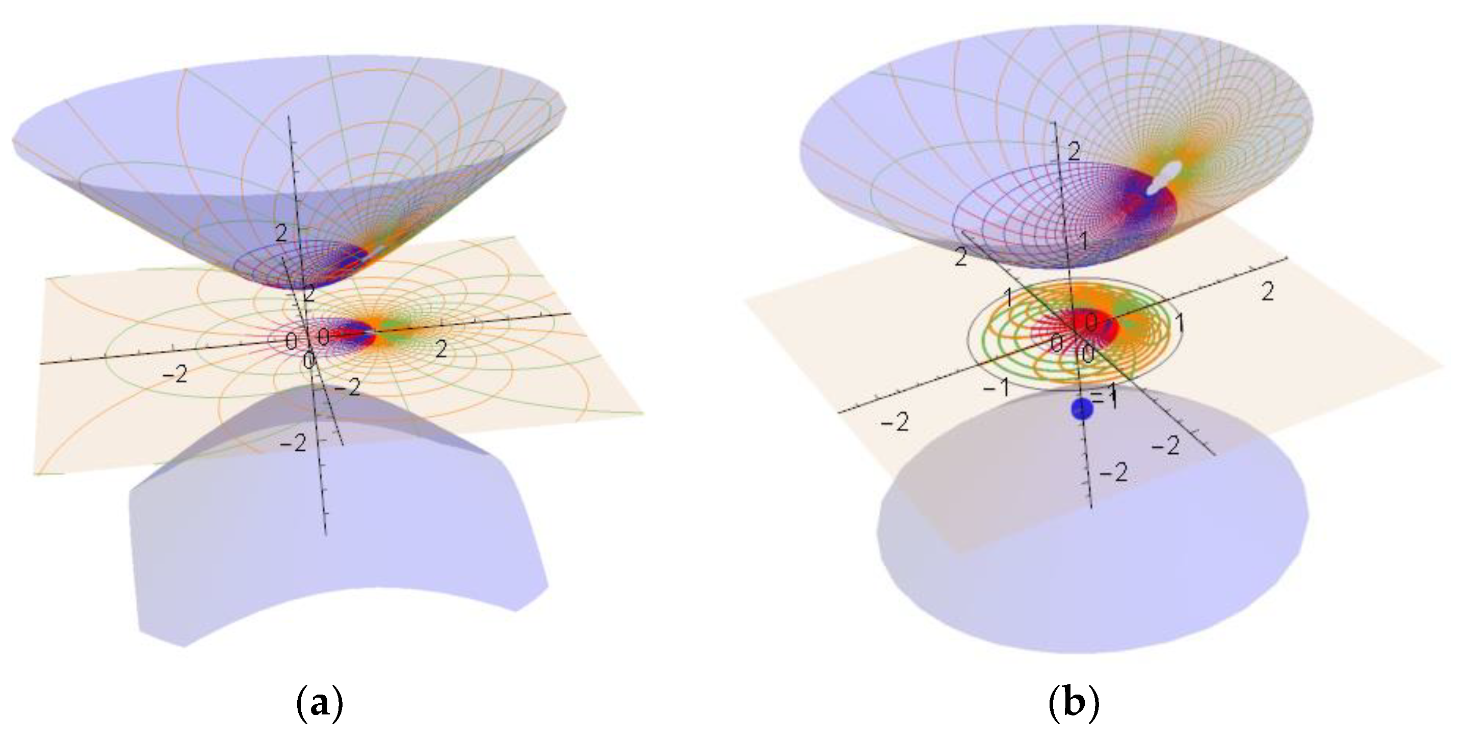
3D Smith Chart and Infinity
To construct the 3D Smith chart [
7,
8,
9,
10] we place the extended Smith chart inside the equatorial plane of the Riemann sphere (
Figure 3) and using the south pole we map it on the unit sphere (
Figure 4):
The 3D Smith chart [
20] obtained in
Figure 4 has a variety of convenient attributes analogous to a real Earth globe, as can be summarized in
Table 1.
In
Figure 5 we can see the idea of infinity more humanly. A girl and a boy start from the centre of the chart moving on the ordinate of the reflection plane (
). When they reach the contour (
), their journey ends and they can never meet again (and just imagine meeting again at infinity). On the 3D Smith chart, once they reach the equator they can continue walking on the same great circle and still meet at infinity (south pole) which is compact and reachable.
We consider the stereographic projection, by using the south pole
on the complex plane
, where
represent the surface of the unit sphere:
This transformation is a bijection and by applying the inverse to the
ρ-plane, then the equations of the 3D Smith chart are presented by:
In the same way, by applying first the Möbius transformation (1) and then
(8), we calculate the corresponding point in the 3D Smith chart of each point
. This is just:
Conversely, a given point on the unit sphere
(i.e.,
) is mapped to in the
ρ-plane (i.e., the sphere equatorial plane) by:
Then, the reflection coefficient magnitude is connected to the coordinate
of the sphere and the phase of the reflection coefficient is equal to the angle of the point
with respect to the sphere
axis:
Similarly,
is mapped into in the z-plane, considering
(6), by:
3. A Hyperbolic Smith Chart
Here we present the mathematical theory that lies behind the intuitive models that we have presented in References [
13,
14].
The extended complex
ρ-plane (
Figure 1c) includes also the loads outside the unit circumference
but thrown also towards infinity and the compact representation requires a sphere) (
Figure 4), which necessitates a software tool for its practical use.
In this hyperbolic approach while maintaining a flat surface, we use models associated to the hyperbolic geometry, the Weierstrass Model and its stereographic projection onto the Poincaré unit disk in the plane [
15].
We consider extended complex
ρ-plane and map it onto the superior part of two sheet hyperboloid using the usual parametrization of this surface. Then, by using the stereographic projection from the upper sheet hyperboloid onto the unit disc
(used in the Poincaré unit disc model of hyperbolic geometry), we construct the Hyperbolic Smith chart (
Figure 6 and
Figure 7).
A generic
ρ-plane point
is mapped on
by the usual parametrization of this surface
:
Next, by applying the stereographic projection
from the point
on the complex plane to a generic point in the space
, we obtain that the point is mapped into the unit disc
centered on the origin, as in the
Figure 6:
Therefore, the hyperbolic Smith chart equation in terms of the voltage reflection coefficients is given by:
By arithmetical manipulations we can further get the connection to the resistance
r and reactance
x:
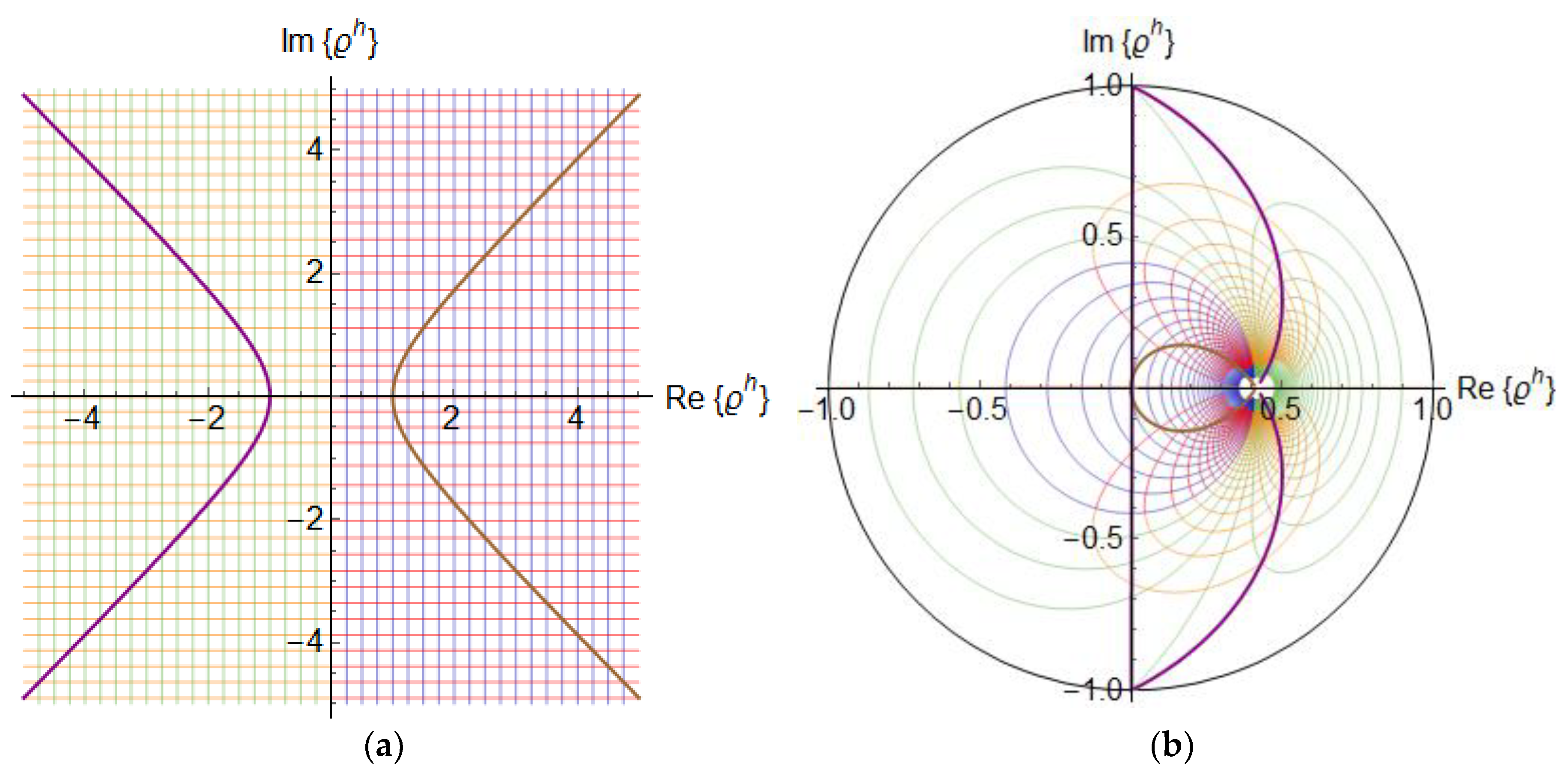
In
Figure 7, we observe the different steps in the construction of the Hyperbolic Generalized Smith chart: First, the generalized Smith chart is sent by
t (14) on the upper sheet of the hyperboloid and then the stereographic projection
(15) send it in the Poincaré unit disc model.
Conversely, a generic point
, in the unit disc centred on the origin, then,
, is mapped through the inverse stereographic projection
into a point in the upper hyperboloid:
Next, this point in the upper hyperboloid is mapped into
by applying the orthogonal projection
. Therefore, a given generic point
in the Hyperbolic Smith chart is mapped to the
ρ-plane by:
To find the expression in the
z-plane, we need to consider (19) and the extended transformation
(6)
. Then:
4. Properties
The Hyperbolic Smith chart has useful properties. In this section, we summarize them (
Figure 8). The entire Smith chart is mapped into the interior of the 0.414 radius circle of the hyperbolic chart.
The circumference of radius one in the ρ-plane, is mapped by (16) to the circumference of radiu in the ph-plane, |ph| = 0.414 and |ph| = 0 in |ph| = 0.
The Hyperbolic Smith chart contains the circuits with inductive reactance above the horizontal (real line) of the
ρh-plane and the circuits with capacitive reactance below the real line of the hyperbolic reflection plane, like in the Smith chart. Further, as seen from (16), the constant reflection coefficients circles
of the 2D Smith chart are projected onto circles with
in the hyperbolic reflection coefficients plane. The
constant circles (which are exterior to the 2D Smith chart or in the South hemisphere on the 3D Smith chart) and which are important in active circuit design are contained in limited region of the hyperbolic reflection coefficients plane with
, as shown in
Figure 9, and their circular forms is unaltered. The image of the infinite magnitude constant reflection coefficient circle
unimaginable to represent even on a generalized 2D Smith chart becomes the contour of the new chart
.
If we consider lines of constant resistance equal to
in the
z-plane,
we obtain in the
ρh-plane the part inside of the unit circle of the quartic curve:
and in the same way if we consider lines of constant reactance
x =
k in the
z-plane we get in the
ρh-plane the part inside of the unit circle of the quartic curve:
as shown in
Figure 10. These quartic curves are orthogonal along the curve in
ρh-plane, corresponding to the image of the hyperbola
in the
z-plane.
In the hyperbolic Smith chart, by using (19) we see that the reflection coefficient is:
We observe that the phase of the reflection coefficient is the same in the ρ-plane and the ρh-plane and the magnitudes are clearly related.
By using (20), we obtain that the normalize impedance is:
5. Application Example and Discussion
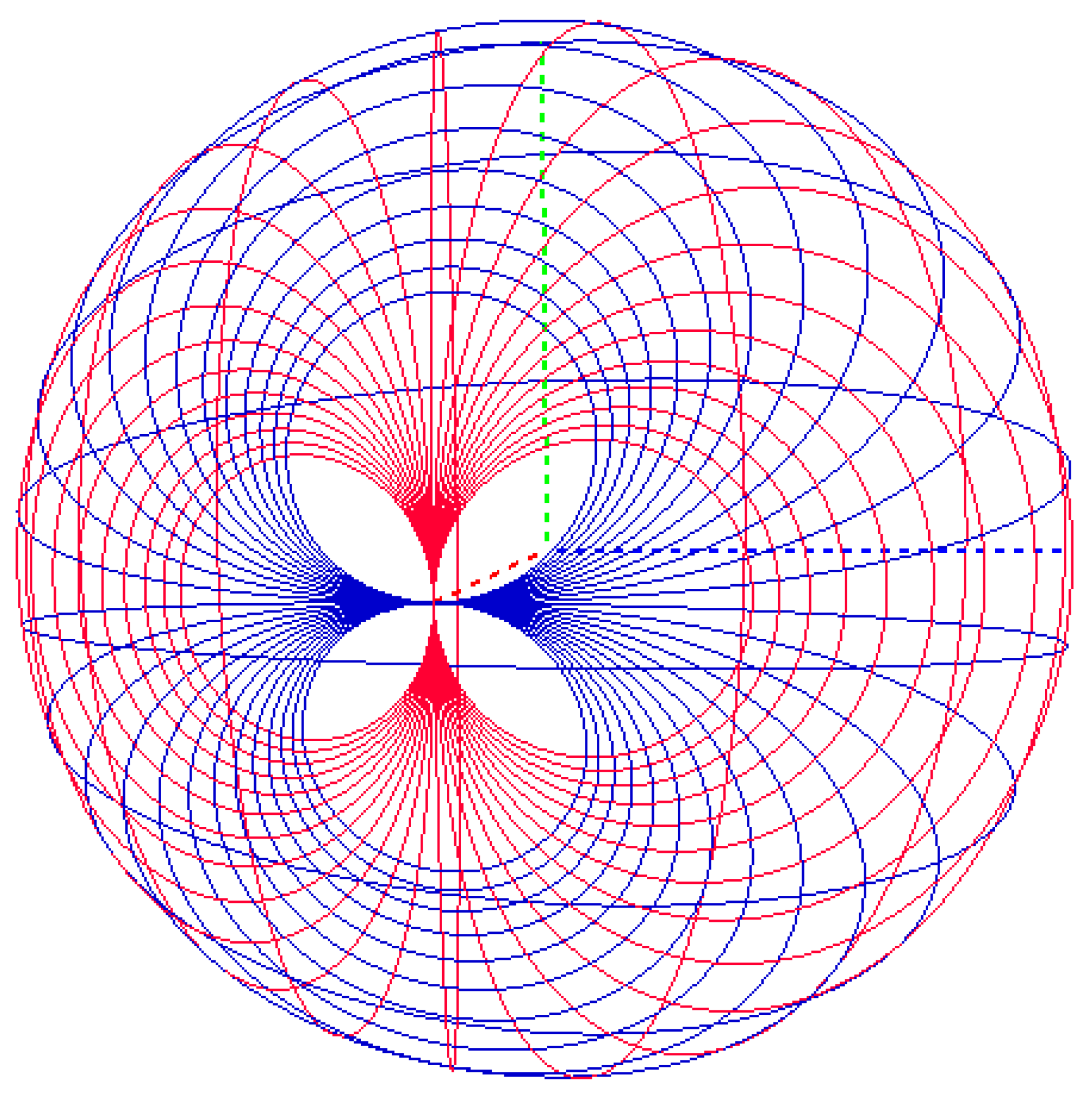
In oscillator theory, the active circuit must exhibit an infinite value of the reflection coefficient at the desired frequency. Surely, the use of a 2D Smith chart based on Euclidean geometry is unattainable to visualize the phenomenon (as seen in
Figure 11).
In the hyperbolic reflection plane, governed by Non-Euclidean geometry [
16] this phenomenon is easy to be seen in
Figure 12a, while in
Figure 12b on the 3D Smith chart.
The hyperbolic Smith chart (whose main properties are summarized in
Table 2) maps the infinite mismatch into the contour of the unit circle, thus if one would use a new vocabulary when passing from one geometry to another [
18] one can translate infinite reflection coefficient (Smith chart) into the proper representation (
Table 3).
6. Conclusions
We have presented the geometric properties of the Smith chart, 3D Smith chart and Hyperbolic Smith chart by means of inversive geometry and hyperbolic geometry.
The infinite magnitude of the reflection coefficient is mapped by these charts (drawn when applied to the grid of the normalized impedance plane) into different locations: infinity on the 2D Smith chart, South pole on the 3D Smith chart and contour of the unit disc for the Hyperbolic Smith chart.
Further we presented for the first time the equations of the Hyperbolic Smith chart, diagram which was previously just intuitively drawn.
The infinity treatment exceeds the classical electrical engineering books and is based on applied pure mathematics (and not engineering manipulations of equations).
In the future, the topology of the 3D Smith chart in particular can be expanded to deal with more complex phenomenon such as phase change materials [
21,
22] where their physical properties vary a lot as frequency or temperature changes. The compact (spherical) representation of its reflection coefficients on its surface leaves the space surrounding it free to be used for visualizing other parameters by employing 3D Euclidean geometry or space filling concepts where the notion of infinity may be treated differently.

 ,
, 


