Abstract
An aggregation operator performs the task of fusing multiple sources of information, which plays a pivotal part in realizing a collective opinion in most decision-making activities. Considering the increasing complexity of decision-making situations, it is imperative to extend aggregation operators for fusing uncertain information with the different forms of attribute values. This study focuses on the development of picture fuzzy sets and aims to design a managerial decision-making solving method. Some operational principles of hesitant picture 2-tuple linguistic variables on account of the Archimedean t-norm and t-conorm are initiated, on which two hesitant picture 2-tuple linguistic weighted operators are established by taking various weight forms. Moreover, we explore the aggregation operators’ idempotency, boundedness, and monotonicity, as well as analyze some particular forms of these operators. Furthermore, these aggregation operators are employed to design a method of deriving an overall performance from evaluation of experts with hesitant picture 2-tuple linguistic terms. An example of selecting service outsourcing supplier is carried out to show the procedures of decision-making with a detailed comparative analysis.
1. Introduction
Decision-making is a common practical activity. One of its aims is to identify the optimal option from several feasible alternatives. There are plenty of plans that involve making choices in our daily life, such as choosing a university to study abroad, recruiting excellent staff, and choosing a suitable career. Decision information is mainly derived from the preferences and judgment information of decision-makers. In the decision-making process, how to describe and fuse the judgment information of experts are two key issues. There has been an aggregation of approaches for forming preferences, which have been developed from different aspects.
In traditional decision-making approaches, decision-makers quantify their preference for each alternative in the form with precise numerical values on the feasible alternatives. Numerical representation methods play pivotal roles in characterizing the preferences of decision-makers with simple forms, which are easy to be calculated. Due to the increasing amount of uncertain and complex information in the decision-making environment, we require to deal with various uncertain types of information, which can include incomplete, imprecise, and even conflicting information [1,2,3]. Since numerical measures are insufficient for describing complex uncertainty or users’ preferences, one tends to evaluate alternatives in the form of natural language. When evaluating many multi-attribute decision-making (MADM) issues, experts are more likely to adopt linguistic values, such as ‘general’, ‘good’, and ‘very good’, to express their opinions. For example, online shopping has increased annually with the use of the Internet, and customers might rate their satisfaction with responses regarding the following aspects: high quality, high speed of delivery, convenient, and easy to return and exchange [4,5]. As shown above, customers usually express their preference information with fuzzy linguistic terms instead of numerical values. With the advent of such applications, the expression and analysis of uncertainty with linguistic terms can assist experts in making intelligent decisions by simulating human cognitive information [6,7,8,9].
Several types of fuzzy set-based methods have been introduced to better describe the judgments and preferences of experts in the form of linguistic terms. Two kinds of typical methods for capturing uncertainty information are symbolic computational methods [10,11,12,13,14] and membership function methods [15,16,17,18,19,20]. Symbolic computational methods describe linguistic terms by introducing ordinal labels and their operational principles. Membership function methods perform a cardinal representation of the linguistic term by establishing a one-to-one correlation between the initial linguistic terms and fuzzy sets. Semantically, compared with the methods mentioned later, these former methods are simpler and more direct, however, because they take a predefined linguistic term as the final operational result. This may cause information loss [21]. To address this issue, linguistic term sets and real numbers (or membership functions) have been integrated to design new methods aligning with the way of human decision-making presentation. In addition, they bring some new fusion techniques of symbolic computational methods in solving decision-making problems [22,23]. 2-Tuple linguistic variables, coined by Herrera and Martínez [24], consist of a symbolic linguistic element and a real number, which can characterize the expert’s preference with consecutive linguistic information and they can effectively avert the information loss and distortion. The 2-tuple linguistic method has been widely employed to address decision-making problems in various fields [25].
In our daily lives, situations exist that demand human opinions including more types of answers: yes, abstain, no, refusal. For example, consider an example of ten board members voting on a candidate for chairman. The voting results are divided into four groups: four suggest agreement, three offer disagreement, two choose abstaining, and one selects refusal [26]. To solve the above-mentioned situation, picture fuzzy set (PFS) was coined by Cuong [27], in which every element is associated with three functions and they can characterize the grades of membership from different aspects. Differing from traditional fuzzy sets and intuitionistic fuzzy sets, PFS performs capturing human decision opinions with more answers in the process of solving a particular problem. The main condition of PFS is that the sum of the three degrees is not to exceed one, and thus we also regard PFS as a standard neutrosophic set [28]. The development of PFS comes with a variety of progress in both new theories and practical applications. Thão and Dinh [29] studied the approximation properties of PFS by combining rough sets, which provides a new perspective for exploring the set properties of PFS. Wei [30] presented some flexible ways to deal with decision-making problems by establishing eight similarity measures between PFSs. Le et al. [31] established an original PFS inference system that improves the reasoning performance of traditional fuzzy inference systems. Dutta and Ganju [32] applied the interval-valued picture fuzzy sets to medical diagnosis based on the distance measure, which offers a new method for capturing and solving uncertainty information in clinical research.
In essence, PFS is a representation method of cognitive information based on membership functions. However, assigning values to portray the cognitive information accurately is a challenging task. In many decision-making activities, some linguistic terms are more suitable to depict the subjective imprecision of human cognition. To take full advantage of PFS and linguistic variables, Wei [33] proposed picture 2-tuple linguistic set (P2TLS), which is suitable to describe the decision-makers’ confidence level. Subsequently, the pertinent information fusion mechanism and comparison principals of P2TLS are explored in [34,35,36]. Although P2TLS has successfully addressed some decision-making problems, they still have room to enhance their effectiveness in some complex decision-making situations. P2TLS is considered as a representation mechanism of single-value information that fails to characterize the hesitant cognitive information when decision-makers facing complex situations. In this study, to deal with this issue, we introduce the concept of hesitant picture 2-tuple linguistic set (HP2TLS) based on the thoughts of intuitionistic hesitant fuzzy set [37], which not only can decrease the information loss and distortion, but also can express the degree of reliability by introducing the information about decision-makers’ confidence level.
In MADM, aggregation operators can be used to fuse different experts’ evaluation information to a group opinion or integrate values concerning different attributes into an overall performance. Different aggregation operators have been developed to serve as the corresponding specific functions, and a slew of aggregation operators have arisen within different situations. Some weighted geometric aggregation operators of 2-tuple linguistic sets were offered in [38], in which both the weights and the attribute preference values are in the form of 2-tuple linguistic information. Xu and Wang [39] introduced some power aggregation operators for taking into account the influence of all arguments under the environment of 2-tuple linguistic variables. Ge and Wei [40] came up with the hesitant 2-tuple weighted aggregation operators in the context of hesitant 2-tuple linguistic information, which consider both the weight of the linguistic information and the position weight. Wang et al. [41] considered the interrelationship of attributes and the prioritization relationship of experts in the process of decision-making by deducing the prioritized and correlated aggregation operators of hesitant 2-tuple linguistic terms. The Archimedean t-norm and t-conorm [42,43] can generalize most of the existing t-norms and t-conorms, such as algebraic and Einstein t-norms and t-conorms [44], which can be used to address the different relationships of aggregated arguments under different attributes’ values including intuitionistic fuzzy sets [45], intuitionistic fuzzy numbers [46], interval-valued fuzzy terms [47,48], single-values neutrosophic numbers [44] and 2-tuple linguistic information [49], etc. To develop more general forms of information fusion mechanisms for hesitant picture 2-tuple variables, this study is concerned with establishing new operational principles for hesitant picture 2-tuple linguistic variables and developing two aggregation operators based on Archimedean t-norm and t-conorm (ATS-HP2TWA operator, ATS-HP2TLWG operator). In addition, we introduce four specific examples of ATS-HP2TLWA and ATS-HP2TLWG operator by taking diverse forms of two auxiliary functions and develop a novel approach to address a practical MADM problem within the hesitant picture 2-tuple situation. The designed decision-making method can provide more choices for the decision-makers in the process of decision-making for reflecting their preferences in choosing aggregation functions.
The remainder of this paper is structured as follows: Section 2 presents some fundamental concepts about P2TLS and Archimedean operators. Then, we introduce the definition of HP2TLS based on P2TLS. In Section 3, some new operational principles and pertinent theorems about HP2TLS are proposed. In Section 4, some aggregation operators are introduced. In addition, their pertinent properties are also demonstrated. In Section 5, we come up with a method for MADM problems under the situation of the HP2TLS. Moreover, a detailed example is given to explain the applicability and flexibility of the aforementioned method in Section 6. Some conclusions are drawn in the final section.
2. Preliminaries
In MADM problems solving, a linguistic label with an ordered structure is usually predefined to act as a reference quantitative scale. is a collection of linguistic labels, where is a linguistic variable and satisfies the following order relationships: , iff and negative relationship for . To address MADM problems, Herrera and Martinez [24,25,50] introduced a novel model called 2-tuple linguistic term, which is made up of a pair of numbers , where and represents a real number within . When the aggregated value does not precisely match the , denotes the difference between the aggregated value and [24].
Definition 1.
Let σ be a real number in . σ and the 2-tuple linguistic term can be transformed by using the functions and , which are given below [51]:
The element of the linguistic label collection can be transformed into a 2-tuple linguistic term: [52]. In 2017, Wei [38] put forward the fundamental idea of P2TLS, which combines PFSs [27] and 2-tuple linguistic terms for characterizing uncertainty information.
Definition 2.
Let b be a P2TLS in universe X, which is defined below [33]:
where and . , and are all in the unit interval with . , and represent the grades of memberships of x to from positive, neutral and negative aspects, respectively.
For the sake of simplicity, is called a picture 2-tuple linguistic element, where , , , , and . The collection of forms a HP2TLS, denoted as , and stands for the elements’ number of b.
Definition 3.
Let be a HP2TLS, the score function of b is described as follows:
Definition 4.
Let be a HP2TLS, the accuracy function of b is given below:
Definition 5.
Let b and e be two hesitant picture 2-tuple linguistic sets (HP2TLSs) on , the detailed formulas determining the order relation between b and e are listed below:
- (1)
- if SC(b) < SC(e), then b < e,
- (2)
- if SC(b) > SC(e), then b > e,
- (3)
- when SC(b) = SC(e), and
- (a)
- AC(b) = AC(e), then b = e,
- (b)
- AC(b) < AC(e), then b < e,
- (c)
- AC(b) > AC(e), then b > e.
3. Operational Laws of Hesitant Picture 2-Tuple Linguistic Sets
Archimedean t-norm and t-conorm emerge as the extended forms of binary operations that can induce some aggregation operators to fuse imprecise information by taking diverse forms of the additive function and its dual function [53].
Definition 6.
is called a t-norm, when Ψ meets the following four requirements, for any z, , u, [42,43]:
- .
- .
- .
- If , , then .
Definition 7.
is called a t-conorm, when Φ meets the following four requirements, for any z, , u, [42,43]:
- .
- .
- .
- If , , then .
Definition 8.
If is continuous and for all , then forms the Archimedean t-norm [42,43].
The Archimedean t-norm can be determined by a strictly decreasing additive function , which can be described as follows:
where is an inverse function and . Similarly, the formula of Archimedean t-conorm is expressed below:
where and . Inspired by operational principles in previous publications [45,49], in this paper, we discuss some new operational principles for HP2TLSs. To obtain the simplified operational principles, a one-to-one mapping function is established as follows [49]:
Definition 9.
Let and be two HP2TLSs, the following formulas are considered as their operational principles:
- Addition operation
- Multiplication operation
- Scalar-multiplication operation
- Exponential operation
In the following, some special aggregation operators are explored by taking diverse forms of additive function and its dual function . At the same time, for the sake of simplicity, and are omitted in the operation process of HP2TLSs in the sequel.
Remark 1.
If , , then one has the following results:
- (1)
- (2)
- (3)
- (4)
Remark 2.
If , , then the following equalities hold:
- (1)
- (2)
- (3)
- (4)
Theorem 1.
Let b and be two HP2TLSs, and the fundamental properties of the above-mentioned operational principles are acquired as:
- (1)
- (2)
- (3)
- (4)
- (5)
- (6)
Proof.
- (1)
- (2)
- (3)
By comparing the above equations, we can obtain .
- (4)
- (5)
- Notice that
By comparing the above equations, we can obtain .
- (6)
- Based onthe following formulas are obtained:By using the above equations, we can obtain .
□
4. Some Aggregation Operators of HP2TLSs Based on Archimedean T-norm and T-conorm
In this section, according to the Archimedean t-norm and the t-conorm [42,43], some pertinent aggregation operators are deduced under the context of HP2TLS.
Definition 10.
Let be some HP2TLSs, which are assigned some weights with and , then the Archimedean t-norm and t-conorm based hesitant picture 2-tuple linguistic weighted averaging (ATS-HP2TLWA) operator is as follows:
Theorem 2.
Let be some HP2TLSs; then, the ATS-HP2TLWA operator is formulated below:
where , .
Next, we give a detailed study of the properties of the ATS-HP2TLWA operator.
Theorem 3.
Let be some HP2TLSs. Then, several properties of the ATS-HP2TLWA operator are examined below:
- (1)
- (Idempotency): Let be some HP2TLSs, if all are identical, i.e., , for all i, thenProof.Let and , where , for all , then we have□
- (2)
- (Boundedness): Let be some HP2TLSs, if and , thenwhereProof.Since , and are two increasing functions, and are two decreasing functions, then we have:In the same way, we can obtain , . According to Definition 3, 4, and 5, we can verify that . Similarity, can be proved. Thus, the following inequality holds:□
- (3)
- (Monotonicity): Let and be two HP2TLSs, and , . If any and satisfy , then
Proof.
Since , and are two increasing functions, then and are two decreasing functions. If any and satisfy , then we can obtain the following:
Similarly, we can obtain , , .
According to Definitions (3)–(5), we can get
□
Remark 3.
If , , then the ATS-HP2TLWA operator is simplified to the weighted averaging operator of HP2TLSs (HP2TLWA),
Remark 4.
If , , then the ATS-HP2TLWA operator is simplified to the Einstein weighted averaging operator of HP2TLSs (EHP2TLWA),
Remark 5.
If , and , then the ATS-HP2TLWA operator is simplified to the Hamacher weighted averaging operator of HP2TLSs (HHP2TLWA),
Remark 6.
If , and , then the ATS-HP2TLWA is simplified to the Frank weighted averaging operator of HP2TLSs (FHP2TLWA),
Definition 11.
Let be some HP2TLSs, which are assigned some weights defined in Definition (10), then the Archimedean t-norm and t-conorm based hesitant picture 2-tuple linguistic weighted geometric (ATS-HP2TLWG) operator is as follows:
Theorem 4.
Let be some HP2TLSs, then the ATS-HP2TLWG operator is formulated as follows:
Similarly, we can see that the ATS-HP2TLWG operator meets idempotency, boundedness, and monotonicity as well. Additionally, we explore several particular examples of the ATS-HP2TLWG operator for the diverse forms of function and its dual function .
Remark 7.
If , , then the ATS-HP2TLWG operator is simplified to the weighted geometric operator of HP2TLSs (HP2TLWG),
Remark 8.
If , , then the ATS-HP2TLWG operator is simplified to the Einstein weighted geometric operator of HP2TLSs (EHP2TLWG),
Remark 9.
If , and , then the ATS-HP2TLWG operator is simplified to the Hamacher weighted geometric operator of HP2TLSs (HHP2TLWG),
Remark 10.
If , and , then the ATS-HP2TLWA operator is simplified to the Frank weighted geometric operator of HP2TLSs (FHP2TLWG),
5. A Novel Method of Solving MADM Problems
In this section, the detailed steps of solving MADM problems under the situation of HP2TLS are elaborated. Let be a collection of m alternatives and be a collection of n attributes and its corresponding weight vector defined in Definition (10). Suppose that is the judgment information matrix, where is an HP2TLS that represents the evaluation information of the alternative with regards to the attribute .
Step 1: Obtain the judgment information matrix:
Step 2: Fuse all values of each alternative by using the ATS-HP2TLWA operator or the ATS-HP2TLWG operator. Then, we can obtain the collective results:
or
Step 3: Rank according to descending order with respect to the values derived from Definitions (3)–(5), and the ideal alternative can be derived.
6. Application of the Designed Method and Discussion
We select an example [33] to show the practicality of the designed method. Outsourcing a common business activity in which partial job functions are farmed out to a third party. The scope of internal core technology service outsourcing projects is expanding. When enterprises face competitions and challenges, it is necessary to to collaborate with other parties for sharing the resources and profits. Therefore, choosing the right outsourcing suppliers become a key foundation for enterprises development. This study aims to design a practical method for the identification of technical service outsourcing suppliers under the situation of hesitant picture 2-tuple linguistic information.
There are five potential service outsourcing suppliers for a communications industry . A team of experts is invited for identifying the most appropriate choice from the five possible service outsourcing suppliers by considering four attributes, which include commercial integrity (), technical level (), management quality (), and service performance (). At the same time, the attributes’ weights are set to . Later, based on the judgment information provided by experts, the judgment information matrix can be constructed. The linguistic term set is taken as .
Next, we apply the designed method in Section 5 to solve the above-mentioned problem to obtain the ideal solution.
Step 1: Obtain the judgment information matrix, which is delineated in Table 1.

Table 1.
Hesitant picture 2-tuple linguistic decision matrix.
Step 2: Employ the ATS-HP2TLWA operator or the ATS-HP2TLWG operator to aggregate all attributes of . Then, collective results of the two operators are given in Table 2 and Table 3, separately. Through Table 2, we can find that EHP2TLWA operator is a special form of HHP2TLWA operator. When , HHP2TLWA operator degenerates into an EHP2TLWA operator.
Table 2.
The aggregated information based on the ATS-HP2TLWA operator.
Table 3.
The aggregated information based on the ATS-HP2TLWG operator.
Step 3: Obtain score values and sort the alternatives in accordance with Definitions (3)–(5), and the results of two operators are presented in Table 4 and Table 5, separately.
Table 4.
Rankings of alternatives and score values matrix based on the ATS-HP2TLWA operator.
Table 5.
Rankings of alternatives and score values matrix based on the ATS-HP2TLWG operator
To further explore the effects of a parameter in the HHP2TLWA operator, the FHP2TLWA operator, the HHP2TLWG operator, and the FHP2TLWG operator, we observe changes of score values with increasing, and the analysis results are displayed in Figure 1, Figure 2, Figure 3 and Figure 4, separately.
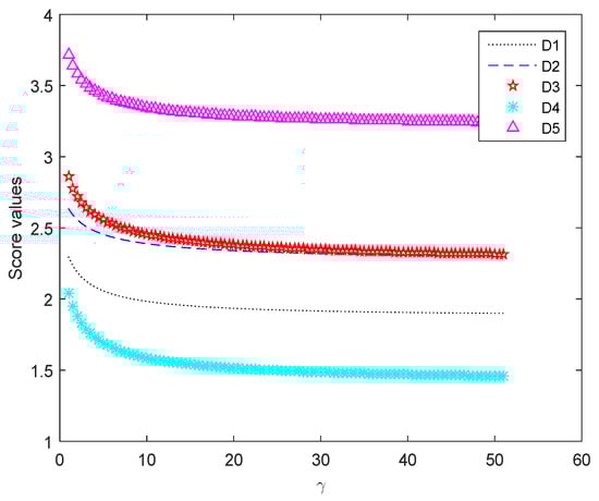
Figure 1.
Variation of ranking with in the HHP2TLWA operator.
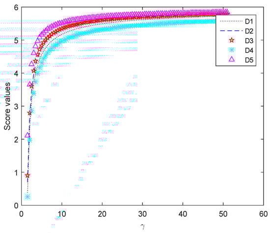
Figure 2.
Variation of ranking with in the FHP2TLWA operator.
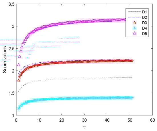
Figure 3.
Variation of ranking with in the HHP2TLWG operator.
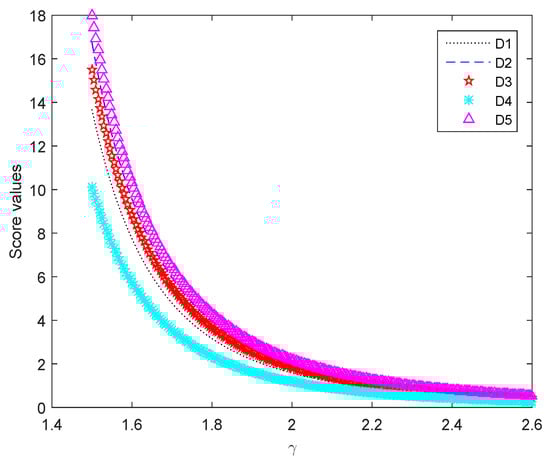
Figure 4.
Variation of ranking with in the FHP2TLWG operator.
In Figure 1, the score values of the alternatives, which are received by the HHP2TLWA operator, keep a smaller variability. As is increasing from 1 to 51, we indicate that score values of the five alternatives are decreasing, but the ranking results always keep . In addition, when is greater than 20, the score values of and are almost overlapping. Figure 2 displays the score values of each alternative derived from the FHP2TLWA operator. As is increasing from 1 to 51, the score values of alternatives are increasing and keep a greater variability. , , and are almost overlapping, when reaches 30, but the ranking result remains unchanged. Figure 3 represents the changing trajectory of the HHP2TLWG operator score values. All score values of the alternatives are increasing with changing. When reaches 30, and are almost overlapping, but ranking order of the alternatives remains . Figure 4 notes the score values of five alternatives achieved by the FHP2TLWG operator. When the value of is larger than 2.6, the score values of alternatives tend to zero. Therefore, the range of parameter values is between 1.5 and 2.6. By carefully analyzing Figure 4, it can be observed that the higher the value of is, the lower the score values are of each alternative. However, the order of relations among alternatives holds , and when is greater than 2, the score values of , , and are almost overlapping.
From the above analysis, it is clear that the score values of the five alternatives change as changed. However, the ranking results of the alternatives do not change in the HHP2TLWA operator, the FHP2TLWA operator, HHP2TLWG operator and the FHP2TLWG operator. Consequently, this means that the ranking result basically remains constant with the parameter changing in the preceding four operators.
7. Conclusions
In this study, we extended the Archimedean t-norm and t-conorm into the context of HP2TLS, aimed at developing the approaches of information fusion with HP2TLSs. Firstly, some new operational principles about HP2TLSs were derived. Subsequently, we introduced two new aggregation operators, called the ATS-HP2TLWA operator and the ATS-HP2TLWG operator, based on new operational principles. In addition, we demonstrated the aggregation operators’ properties. Meanwhile, some specific examples were examined based on assigning different functions in the ATS-HP2TLWA and the ATS-HP2TLWG operators. A method for identifying the ideal alternative was also designed regarding the introduced operators. A single example was applied to highlight the applicability and flexibility of the improved decision-making method. Futhermore, in four specific aggregation operators, we gave a detailed discussion comparing the changing trends of the score values and the ideal option with changing.
Author Contributions
Funding acquisition, L.W. and X.F.; Methodology, Y.W.; Supervision, L.W.; Validation, X.F. and H.W.; Visualization, H.W.; Writing-original draft, Y.W.; Writing-review & editing, L.W. and X.F.
Funding
This work is supported by the Natural Science Foundation of China (Nos. 61773352, 61803065), the National Nuclear Energy Development Project of China (No. 18zg6103), the Science and Technology Planning Project of Sichuan Province (2018JY0522) and the Fundamental Research Funds for the Central Universities (Nos. 3132018225, 3132016306).
Conflicts of Interest
The authors declare no conflict of interest.
References
- Park, J.H.; Kwun, Y.C.; Son, M.J. A generalized intuitionistic fuzzy soft set theoretic approach to decision making problems. Int. J. Fuzzy Logic Intell. Syst. 2011, 11, 71–76. [Google Scholar] [CrossRef]
- Xiao, G.Q.; Li, K.L.; Li, K.Q. Reporting/most influential objects in uncertain databases based on probabilistic reverse top-k queries. Inf. Sci. 2017, 405, 207–226. [Google Scholar] [CrossRef]
- Xiao, G.Q.; Li, K.L.; Zhou, X.; Li, K.Q. Efficient monochromatic and bichromatic probabilistic reverse top-k query processing for uncertain big data. J. Comput. Syst. Sci. 2017, 89, 92–113. [Google Scholar] [CrossRef]
- Shenbaga, T.S. A study on the customer satisfaction towards online shopping. Sumedha J. Manag. 2015, 4, 4–15. [Google Scholar]
- Trong, V.H.; Tan, N.; Khanh, V.; Gim, G. Evaluating factors influencing consumer satisfaction towards online shopping in viet nam. J. Emerg. Trends Comput. Inf. Sci. 2014, 5, 67–71. [Google Scholar]
- Akusok, A.; Miche, Y.; Hegedus, J.; Rui, N.; Lendasse, A. A two-stage methodology using K-NN and false-positive minimizing ELM for nominal data classification. Cognit. Comput. 2014, 6, 432–445. [Google Scholar] [CrossRef]
- Czubenko, M.; Kowalczuk, Z.; Ordys, A. Autonomous driver based on an intelligent system of decision-making. Cognit. Comput. 2015, 7, 569–581. [Google Scholar] [CrossRef] [PubMed]
- Meng, F.Y.; Chen, X.H. Correlation coefficients of hesitant fuzzy sets and their application based on fuzzy measures. Cognit. Comput. 2015, 7, 445–463. [Google Scholar] [CrossRef]
- Yang, J.; Gong, L.Y.; Tang, Y.F.; Yan, J.; He, H.B.; Zhang, L.Q.; Li, G. An improved SVM-based cognitive diagnosis algorithm for operation states of distribution grid. Cognit. Comput. 2015, 7, 582–593. [Google Scholar] [CrossRef]
- Herrera, F.; Herrera-Viedma, E. Choice functions and mechanisms for linguistic preference relations. Eur. J. Oper. Res. 2000, 120, 144–161. [Google Scholar] [CrossRef]
- Herrera, F.; Herrera-Viedma, E. Linguistic decision analysis: Steps for solving decision problems under linguistic information. Fuzzy Sets Syst. 2000, 115, 67–82. [Google Scholar] [CrossRef]
- Herrera, F.; Herrera-Viedma, E.; Verdegay, J.L. A model of consensus in group decision making under linguistic assessments. Fuzzy Sets Syst. 1996, 78, 73–87. [Google Scholar] [CrossRef]
- Wu, Q.; Wang, F.; Zhou, L.G.; Chen, H.Y. Method of multiple attribute group decision making based on 2-dimension interval type-2 fuzzy aggregation operators with multi-granularity linguistic information. Int. J. Fuzzy Syst. 2017, 19, 1880–1903. [Google Scholar] [CrossRef]
- Xu, Z.S. A method based on linguistic aggregation operators for group decision making with linguistic preference relations. Inf. Sci. 2014, 166, 19–30. [Google Scholar] [CrossRef]
- Atanassov, K.T. Intuitionistic fuzzy sets. Fuzzy Sets Syst. 2012, 20, 87–96. [Google Scholar] [CrossRef]
- Kim, T.; Sotirova, E.; Shannon, A.; Atanassova, V.; Atanassov, K.; Jang, L. Interval valued intuitionistic fuzzy evaluations for analysis of a student’s knowledge in university e-learning courses. Int. J. Fuzzy Logic Intell. Syst. 2018, 18, 190–195. [Google Scholar] [CrossRef]
- Qin, J.D.; Liu, X.W.; Pedrycz, W. A multiple attribute interval type-2 fuzzy group decision making and its application to supplier selection with extended LINMAP method. Soft Comput. 2017, 21, 3207–3226. [Google Scholar] [CrossRef]
- Xia, M.M.; Xu, Z.S. Hesitant fuzzy information aggregation in decision making. Int. J. Approx. Reason. 2011, 52, 395–407. [Google Scholar] [CrossRef]
- Xia, M.M.; Xu, Z.S.; Chen, N. Some hesitant fuzzy aggregation operators with their application in group decision making. Group Decis. Negot. 2013, 22, 259–279. [Google Scholar] [CrossRef]
- Zadeh, L.A. Fuzzy Sets, Fuzzy logic, & Fuzzy Systems. Fuzzy Sets 1996, 8, 394–432. [Google Scholar]
- Martínez, L.; Rodriguez, R.M.; Herrera, F. The 2-Tuple Linguistic Model-Computing with Words in Decision Making; Springer Publishing Company: New York, NY, USA, 2015. [Google Scholar]
- Chen, Z.C.; Liu, P.H.; Pei, Z. An approach to multiple attribute group decision making based on linguistic intuitionistic fuzzy numbers. Int. J. Comput. Intell. Syst. 2015, 8, 747–760. [Google Scholar] [CrossRef]
- Wang, J.Q.; Li, H.B. Multi-criteria decision-making method based on aggregation operators for intuitionistic linguistic fuzzy numbers. Control Decis. 2010, 25, 1571–1574. [Google Scholar]
- Herrera, F.; Martinez, L. A 2-tuple fuzzy linguistic representation model for computing with words. IEEE Trans. Fuzzy Syst. 2000, 8, 746–752. [Google Scholar]
- Herrera, F.; Martinez, L. A model based on linguistic 2-tuples for dealing with multigranular hierarchical linguistic contexts in multi-expert decision-making. IEEE Trans. Syst. Man Cybern. Part B Cybern. 2000, 31, 227–234. [Google Scholar] [CrossRef] [PubMed]
- Wang, R.; Li, Y.L. Picture hesitant fuzzy set and its application to multiple criteria decision-making. Symmetry 2018, 10. [Google Scholar] [CrossRef]
- Cuong, B.C. Picture fuzzy sets-first results: Part 1. J. Comput. Sci. Cybern. 2014, 30, 409–420. [Google Scholar]
- Cuong, B.C.; Prhong, P.H.; Smarandache, F. Smarandache. Standard neutrosophic soft theory: Some first results. Neutrosophic Sets Syst. 2016, 12, 80–91. [Google Scholar]
- Thão, N.X.; Dinh, N.V. Rough picture fuzzy set and picture fuzzy topologies. J. Comput. Sci. Cybern. 2015, 31, 245–253. [Google Scholar]
- Wei, G.W. Some cosine similarity measures for picture fuzzy sets and their applications to strategic decision making. Informatica 2017, 28, 547–564. [Google Scholar] [CrossRef]
- Le, H.S.; Viet, P.V.; Hai, P.V. Picture inference system: A new fuzzy inference system on picture fuzzy set. Appl. Intell. 2017, 46, 652–669. [Google Scholar]
- Dutta, P.; Ganju, S. Application of interval valued picture fuzzy set in medical diagnosis. In Proceedings of the 19th International Conference on Knowledge Discovery and Fuzzy Systems, Mumbai, India, 7–8 February 2017. [Google Scholar]
- Wei, G.W. Picture 2-tuple linguistic Bonferroni mean operators and their application to multiple attribute decision making. Int. J. Fuzzy Syst. 2017, 19, 997–1010. [Google Scholar] [CrossRef]
- Nie, R.X.; Wang, J.Q.; Wang, T.L. A hybrid outranking method for greenhouse gas emissions’ institution selection with picture 2-tuple linguistic information. Comput. Appl. Math. 2018. [Google Scholar] [CrossRef]
- Wei, G.W.; Alsaadi, F.E.; Hayat, T.; Alsaedi, A. Picture 2-tuple linguistic aggregation operators in multiple attribute decision making. Soft Comput. 2018, 22, 989–1002. [Google Scholar] [CrossRef]
- Zhang, X.Y.; Wang, J.Q.; Hu, J.H. On novel operational laws and aggregation operators of picture 2-tuple linguistic information for MCDM problems. Int. J. Fuzzy Syst. 2018, 20, 958–969. [Google Scholar] [CrossRef]
- Beg, I.; Rashid, T. Group decision making using intuitionistic hesitant fuzzy sets. Int. J. Fuzzy Logic Intell. Syst. 2014, 14, 181–187. [Google Scholar] [CrossRef]
- Wei, G.W. A method for multiple attribute group decision making based on the ET-WG and ET-OWG operators with 2-tuple linguistic information. Exp. Syst. Appl. 2010, 37, 7895–7900. [Google Scholar] [CrossRef]
- Xu, Y.J.; Wang, H.M. Approaches based on 2-tuple linguistic power aggregation operators for multiple attribute group decision making under linguistic environment. Soft Comput. 2011, 11, 3988–3997. [Google Scholar] [CrossRef]
- Ge, S.N.; Wei, C.P. A hesitant fuzzy language decision making method based on 2-tuple. Oper. Res. Manag. Sci. 2017, 26, 108–114. (In Chinese) [Google Scholar]
- Wang, L.D.; Wang, Y.J.; Liu, X.D. Prioritized aggregation operators and correlated aggregation operators for hesitant 2-tuple linguistic variables. Symmetry 2018, 10. [Google Scholar] [CrossRef]
- Klir, G.J.; Yuan, B. Fuzzy sets and fuzzy logic: Theory and applications. Prent. Hall 1995, 1, 283–287. [Google Scholar]
- Nguyen, H.T.; Walker, E.A. A First Course in Fuzzy Logic; CRC Press: Boca Raton, FL, USA, 1997. [Google Scholar]
- Liu, P.D. The aggregation operators based on Archimedean t-conorm and t-norm for single-valued neutrosophic numbers and their application to decision making. Int. J. Fuzzy Syst. 2016, 18, 849–863. [Google Scholar] [CrossRef]
- Xia, M.M.; Xu, Z.S.; Zhu, B. Some issues on intuitionistic fuzzy aggregation operators based on Archimedean t-conorm and t-norm. Knowl. Based Syst. 2012, 31, 78–88. [Google Scholar] [CrossRef]
- Liu, P.D.; Chen, S.M. Heronian aggregation operators of intuitionistic fuzzy numbers based on the Archimedean t-norm and t-conorm. In Proceedings of the 2016 International Conference on Machine Learning & Cybernetics, Jeju, Korea, 10–13 July 2016; pp. 686–691. [Google Scholar]
- Yu, D. Group decision making under interval-valued multiplicative intuitionistic fuzzy environment based on Archimedean t-conorm and t-norm. Int. J. Intell. Syst. 2015, 30, 590–616. [Google Scholar] [CrossRef]
- Zhang, Z.M.; Wu, C. Some interval-valued hesitant fuzzy aggregation operators based on Archimedean t-norm and t-conorm with their application in multi-criteria decision making. Int. J. Intell. Syst. 2014, 27, 2737–2748. [Google Scholar]
- Tao, Z.F.; Chen, H.Y.; Zhou, L.G.; Liu, J.P. On new operational laws of 2-tuple linguistic information using Archimedean t-norm and s-norm. Knowl. Based Syst. 2014, 66, 156–165. [Google Scholar] [CrossRef]
- Herrera, F.; Martinez, L. An approach for combining linguistic and numerical information based on the 2-tuple fuzzy linguistic representation model in decision-making. Int. J. Uncertain. Fuzziness Knowl. Based Syst. 2000, 8, 539–562. [Google Scholar] [CrossRef]
- Yang, W.; Chen, Z.P. New aggregation operators based on the Choquet integral and 2-tuple linguistic information. Expert Syst. Appl. 2012, 39, 2662–2668. [Google Scholar] [CrossRef]
- Zhang, W.C.; Xu, Y.J.; Wang, H.M. A consensus reaching model for 2-tuple linguistic multiple attribute group decision making with incomplete weight information. Int. J. Syst. Sci. 2016, 47, 389–405. [Google Scholar] [CrossRef]
- Zhang, Z.M. Archimedean operations-based interval-valued hesitant fuzzy ordered weighted operators and their application to multi-criteria decision making. Br. J. Math. Comput. Sci. 2016, 17, 1–34. [Google Scholar] [CrossRef] [PubMed]


© 2018 by the authors. Licensee MDPI, Basel, Switzerland. This article is an open access article distributed under the terms and conditions of the Creative Commons Attribution (CC BY) license (http://creativecommons.org/licenses/by/4.0/).