A Q-Learning-Based Approach for Deploying Dynamic Service Function Chains

Abstract

As the size and service requirements of today’s networks gradually increase, large numbers of proprietary devices are deployed, which leads to network complexity, information security crises and makes network service and service provider management increasingly difficult. Network function virtualization (NFV) technology is one solution to this problem. NFV separates network functions from hardware and deploys them as software on a common server. NFV can be used to improve service flexibility and isolate the services provided for each user, thus guaranteeing the security of user data. Therefore, the use of NFV technology includes many problems worth studying. For example, when there is a free choice of network path, one problem is how to choose a service function chain (SFC) that both meets the requirements and offers the service provider maximum profit. Most existing solutions are heuristic algorithms with high time efficiency, or integer linear programming (ILP) algorithms with high accuracy. It’s necessary to design an algorithm that symmetrically considers both time efficiency and accuracy. In this paper, we propose the Q-learning Framework Hybrid Module algorithm (QLFHM), which includes reinforcement learning to solve this SFC deployment problem in dynamic networks. The reinforcement learning module in QLFHM is responsible for the output of alternative paths, while the load balancing module in QLFHM is responsible for picking the optimal solution from them. The results of a comparison simulation experiment on a dynamic network topology show that the proposed algorithm can output the approximate optimal solution in a relatively short time while also considering the network load balance. Thus, it achieves the goal of maximizing the benefit to the service provider.

1. Introduction

Currently, most networks use a large number of dedicated hardware devices that provide features such as firewalls and network address translation (NAT). The various services provided by service providers usually require specialized hardware devices. As the network grows in size and emerging industries such as big data [1,2] and cloud computing [3,4,5] are expanding rapidly, starting a new service requires deploying a variety of dedicated hardware devices, making it extremely difficult to design a private protocol and protect the security of user data. Because users share resources on dedicated hardware devices, hackers can take advantage of certain security vulnerabilities in some devices and easily obtain data of users. Nevertheless, as service requirements continue to increase, service providers must regularly expand their physical infrastructure, leading to high infrastructure and operating costs [6,7].

Based on network service requirements, service providers have begun to pay attention to network function virtualization (NFV) technology [8]. Unlike previous dedicated hardware devices, NFV converts network service functions into software, and provides services through a common server device. Although using the same servers, NFV technology isolates the resources and functions on the computer and then allocates them to users, which ensures the privacy and security of user data. Using NFV, service providers can respond quickly to service needs and traffic changes by managing software to distribute services. Moreover, by centralizing resource management, service providers can reduce infrastructure and operating costs [9].

Using NFV technology, we can use virtual network functions (VNFs) [10] to represent network services deployed on continuous network topology nodes to form a service function chain (SFC) [11]. This approach reduces hardware costs and operating expenses but needs to be robust for IT and bandwidth resources [12]. However, the development of NFV also introduces challenges. For example, as user demand grows, the SFC that provides services to the user may need to be adjusted frequently to ensure service continuity, for example, when the user moves. In this case, preserving continuity requires changing the SFC in the network topology to suit the user’s requests [13]. However, an intelligent approach to building and adjusting SFCs to reduce labor costs is worth investigating.

For an SFC, when a service ends, the best deployment for a new request may change [14]. Static SFC deployment causes unnecessary resource consumption and wastes many idle resources. Therefore, dynamic SFC deployment is more suitable for research; we must balance the consumption of various resources in real time.

Reinforcement learning (RL) [15] is an area of machine learning that focuses on determining how software agents should act in an environment to maximize some of the concepts of cumulative rewards. This problem is broad and applicable to many fields [16,17,18,19,20].

RL is also used to study the existence of optimal solutions and accurate algorithm calculation to adapt to and explore unknown environmental models without requiring training data support. In some cases, RL can be used to yield limited-equilibrium decisions. RL refers to an agent in an environment that involves many states. Through RL, each agent learns appropriate actions by receiving rewards for actions taken to achieve its purpose. The states that exist in an environment may or may not help the agent achieve the goal. As agents experience each state while attempting to achieve their goals, they are rewarded by the environment. When an agent consistently fails to reach the target state, it cannot gain the reward. Thus, agents iterate through many trials and errors and eventually learn the most appropriate action for each state.

However, there are many researches related to reinforcement learning, such as stochastic learning automata [21,22], Q-learning [23], deep Q network [24], and Generative Adversarial Networks [25]. After our comparison, we found that Q-learning is most suitable for the problems studied in this paper.

In this study, we use an RL algorithm called Q-learning. The rewards and strategies are recorded in a matrix. The goal of the training phase is to make the strategy that preserves the matrix ($Q$ matrix) converge. The matrix has been proven to converge for continuous decision problems in environments that meet the requirements of RL. During use, the state transition strategy is provided directly by the $Q$ matrix containing the policy.

The reasons why we use Q-learning are as follows. First of all, because a common problem of machine learning is it is time consuming in training; the Q-learning training stage is easy to understand, and the structure of the storage strategy is easy to be modified, so it can be optimized. Secondly, the problem that Q-learning can solve is more similar to the problem in this paper, which helps to give play to the advantages of the algorithm. Therefore, the use of the Q-learning algorithm can greatly reduce the training time and computational complexity.

To optimize the deployment of SFCs in a dynamic network, we integrated RL into the problem and designed a new deployment decision algorithm. This paper studies the problem of deploying SFCs in a multiserver dynamic network. Unlike the data center network [26,27], the nodes of the multi-server network have fewer resources and the SFC deployment is more difficult. Due to the characteristics of dynamic networks, new SFCs may need to be deployed at any time, and some services should be cancelled. To accomplish these tasks, we propose a real-time online deployment decision algorithm called QLFHM. After learning the entire topology and the use of virtual resources, the algorithm uses the RL module and the load balancing module to output an SFC immediately. We compared our proposed algorithm with other algorithms in a simulation experiment and evaluated it repeatedly. The simulation results show that the algorithm achieves good performance with regard to decision time, load balancing, deployment success rate and deployment profit.

The rest of this paper is organized as follows. Section 2 provides an overview of the current work related to the field. In Section 3, we describe the problem models we want to solve, including network models, user requests, and dynamic deployment adjustments. To solve these problems, we propose our algorithm model in Section 4. We present a comparison with other algorithms in Section 5. Finally, Section 6 summarizes the paper.

2. Related Work

In NFV networks, network functions are implemented as VNFs in software form. The characteristics of VNFs allow them to be deployed flexibly and ensure the security of users. Therefore, key consideration needs to be given to the placement of VNFs to meet service requirements, quality of service, and the interests of service providers. This type of problem is called the VNF Placement (VNF-P) problem and has been proven to be a non-deterministic polynomial-time hard (NP-hard) problem [28]. Consequently, it is often difficult to find the optimal solution of a VNF-P problem.

The study of deployment problems is divided into static deployment problems and dynamic deployment problems. The difference is that during static deployment, the SFC in the network is always there; in contrast, during dynamic deployment it will be withdrawn after some period.

In a static problem, deployment is the equivalent of an offline decision: all the requirements are considered when choosing the deployment. Because the SFC being deployed is not retracted after placement, the main consideration is how to arrange more SFCs, which is also the main evaluation criterion. For example, the BSVR algorithm proposed by Li et al. [29] mainly considers load balancing and the number of accepted SFCs. In addition, unlike us, they set up a consistent type of VNF that can be shared by multiple SFCs.

Here, we study the dynamic problem, which is closer to the real network situation [30]. In a dynamic situation, an SFC will be withdrawn after some deployment period, making the network more fluid.

Facing those problems, the methods are similar. To obtain the optimal solution of the VNF-P problem, mathematical programming methods such as integer linear programming (ILP) and mixed ILP (MILP) are the most popular approach [31]. The next most popular approaches involve heuristic algorithms [32] or a combination of heuristic algorithms and ILP. Although there are different optimization approaches to VNF-P problems, the limitations of these approaches are generally similar and include bandwidth resources, IT resources, link delay, VNF deployment, and cost and profit considerations [33,34,35].

For example, Bari et al. [28] approximately expressed the VNF-P problem as an ILP model and solved it with a heuristic algorithm that attempted to minimize operating expense (OPEX) and maximize network utilization. Gupta et al. [33] tried to minimize bandwidth consumption. Luizelli et al. [31] also developed an ILP model that seeks to minimize both the end-to-end delay and the resource overhang ratio. J. Liu et al. [14] proposed the column generation (CG) model algorithm based on ILP and attempted to maximize the service provider’s profit and the request acceptance ratio.

Some of the papers mentioned above have reported that the execution times for solving these two mathematical models increase exponentially with the size of the network. After solving the model with optimization software or a precision algorithm, they immediately proposed a corresponding heuristic algorithm.

Although the execution times of heuristic algorithms is much lower than that of ILP, most existing heuristic algorithms provide only near-optimal solutions. However, considering the time savings, heuristic algorithms form the main approach to solving VNF-P problems.

Some recent solutions to the VNF-P problem have applied machine learning techniques. Kim et al. [36] constructed the entire problem as an RL model. Although the results of this approach may not differ much from the optimal solution, using it in complex network situations results in extremely long training times.

We also tried to avoid the shortcoming of too long training time while using intensive learning. Given the tradeoff between the accuracy of the ILP algorithm and the time efficiency of the heuristic algorithm, this paper proposes a QLFHM algorithm that combines RL and heuristic algorithms. After comparing QLFHM with benchmark algorithms, we conclude that the QLFHM algorithm not only guarantees an approximately optimal solution but also guarantees the time efficiency when dynamically deploying a SFC.

3. Problem Description

We studied the problem of deploying an SFC across multiple servers in a dynamic network. Our goal is to make the service provider most profitable while providing security guaranteed services.

We consider a scenario in which multiple input requests need to be deployed from the source server to the target server over an appropriate link. The link must support the VNFs included in the request. Due to the limited capacity of all servers and links, consideration should be given to the distribution of SFCs to be deployed for the request that will allow more SFCs to be deployed.

We describe the problem model in the next sections, including the research motivation, network model, request model and dynamic SFC deployment.

3.1. Research Motivation

Given a network with multiple servers, and each server supports the deployment of VNFs, but IT resources are limited. Link bandwidth resources are also limited. Requests dynamically switch between active and offline states. Thus, effectively determining how to deploy the SFCs can maximize the request acceptance ratio and the service provider’s profit and minimize the computation time, while satisfying all the constraints.

3.2. Network Model

The network can be seen as a graph $G = \left(V, E\right)$, where $V$ denotes the set of nodes, and $E$ is the set of links between nodes. Each $e\in E$ represents a physical link between two network nodes; we use $B_e\in N$ to show a link’s bandwidth capacity. Each $v\in V$ is a network server, which functions as both the users’ access point and a switch; each server also has an IT resource capacity; we use $I_v\in N$ to denote the IT resources of $v$. $T$ represents the set of all the VNFs. We use $T_v\in T$ to denote the set of VNFs that can be deployed at each $v$. All servers can offer NFV services; however, some servers only support partial services. We assume that bandwidth resources and node computing resources are limited. We use a Boolean variable $p_{j,v}$ to represent the state in which the j-th VNF $vn{f}_j$ is deployed on $v\in V$. A $p_{j,v}$ value of 1 denotes deployable and a value of 0 denotes undeployable:

$$p_{j,v}= \{\begin{array}{c}1 if vn{f}_j\in T_{v },I_v>0\\ 0 else \end{array}$$

(1)

3.3. Request Model

$RE$ is used to represent all incoming requests. Each request $i\in RE$ is represented by the following variables: $s_i, d_i, P_i, r_i$. Here, $s_i\in V$ refers to the client’s access node, $d_i\in V$ is the data provider node required by the user, $P_i\in T$ is a vector that includes the required VNFs sequence on the request SFC, and $r_i\in R^{+}$ refers to the unit compensation paid after the successful deployment of the request, which is related to the number of VNFs represented by $num\_vnf{s}_i$. We use $\omega$ to represent the unit value. For convenience, we make $\omega =1$:

$$r_i= \frac{3}{2}\ast num\_vnf{s}_i \ast \omega .$$

(2)

The profit gained after successful deployment of the SFC of user$i$ is represented by $profi{t}_i$, and $l_i$ represents the chain length of a successfully deployed SFC: the number of nodes in the SFC:

$$profi{t}_i= r_i-l_i \ast \omega .$$

(3)

A successfully deployed $sf{c}_i$ should match the starting point $s_i$ and destination $d_i$, select an appropriate chain, and arrange the VNFs sequence sequentially on the chain nodes. The link length $l_i$ is limited by the compensation $r_i$. Service providers need to ensure their profitability:

$$l_i < \frac{r_i}{\omega }.$$

(4)

$x_i$ is a Boolean variable that indicates whether the request of user $i$ is successfully deployed. If its SFC is online, $x_i$ is 1; otherwise, $x_i$ is 0. $Node\_SF{C}_i$ represents all the nodes in $sf{c}_i$. $Node\_vNF{s}_i$ represents the nodes that can deploy VNFs in $sf{c}_i$. $Link\_SF{C}_i$ represents all the links in the $sf{c}_i$. $z_{i,j,\pi }$ is a Boolean variable that equals 1 if user $i$ uses the path $\pi \in Link\_SF{C}_i$ and the next node that deploys VNFs of its node-deployed j-th VNF is node deployed—the (j + 1)-th VNF—and 0 otherwise.

Equation (5) ensures that the nodes deploying VNFs do not include the user access node $s_i$ or the service access node $d_i$:

$$Node\_vNF{s}_i= Node\_SF{C}_i-\left(s_i+d_i\right).$$

(5)

Equations (6) and (7) ensure that when the $sf{c}_i$ is online, the $P_i$ is deployed in the $sf{c}_i$ in sequence:

$$\underset{v\in Node\_vNF{s}_i}{{\displaystyle \cap }}{p}_{j,v}= x_i, \forall vn{f}_j\in P_i \forall i\in RE$$

(6)

$$\underset{\pi \in Link\_SF{C}_i}{{\displaystyle \cap }}{z}_{i,j,\pi } = x_i ,\forall vn{f}_j\in P_i \forall i\in RE.$$

(7)

3.4. Dynamic SFC Deployment

We assume that during the arrival of a dynamic request scenario, the service provider will provide service for the new request and will cancel the service function of a previous SFC at the end of the service request time. The arrival time of requests occurs at a certain time interval. Therefore, at every moment, the service provider addresses two types of user requests. These mainly affect the service provider’s operation expenses and involve checking whether a new request is available and whether there a chain of online services exists that need to be cancelled.

The goal of dynamic deployment is to maximize service provider profits. The IT resources and bandwidth capacity exist as the deployment constraint condition; however, they affect only the deployment ability and not the operation cost.

$Node\_vNFs\_pu{t}_i$ represents the node set that deployed VNFs for $sf{c}_i$. $I\_ma{x}_v$ represents the maximum IT capacity of node $v$. $I\_us{e}_j$ means the IT capacity needed by j-th VNF. $Link\_vNFs\_pu{t}_i$ is the set of links that belong to $sf{c}_i$. $B\_ma{x}_e$ denotes the maximum bandwidth capacity of link $e$, and $B\_us{e}_i$ is the bandwidth capacity needed by the $sf{c}_i$.

For every $v\in V$:

$$\sum _{i\in RE}{I}_{use}{}_j\ast p_{j,v}\ast x_i \le I\_ma{x}_v , if v\in Node\_vNFs\_pu{t}_i,\forall vn{f}_j\in P_i,$$

(8)

and for every $e\in E$:

$$\sum _{i\in RE}B\_us{e}_i\ast x_i \le B\_ma{x}_e , if e\in Lin{k}_{vNF{s}_{{put}_i}}$$

(9)

Equations (8) and (9) ensure that the user will not use more bandwidth and IT resources than the total capacity available during any service time.

It should be noted, however, that some requests may be blocked because their long deployment chains result in no profits. The Boolean variable $y_i$ indicates whether the request of user $i$ has been successfully deployed. The goal of this problem is to maximize the service provider’s profit $K$, described as follows:

$$K = \sum _{i\in RE}profi{t}_i \ast y_i.$$

(10)

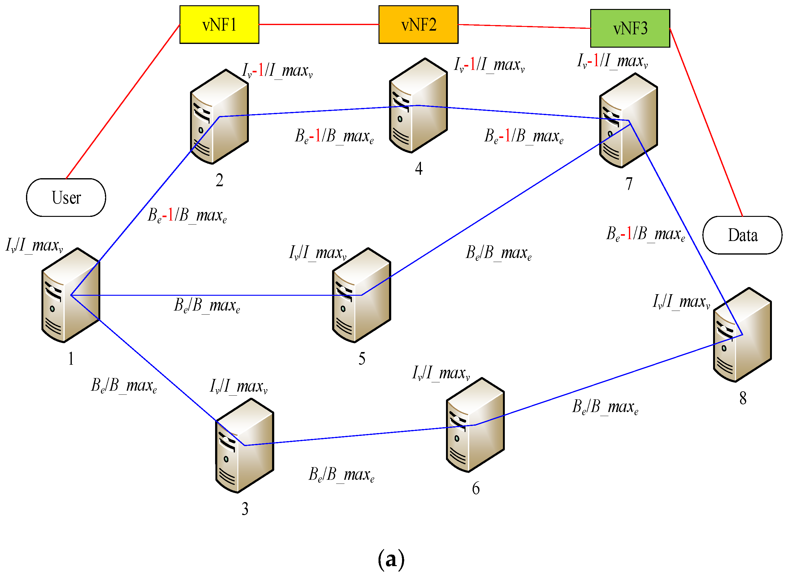
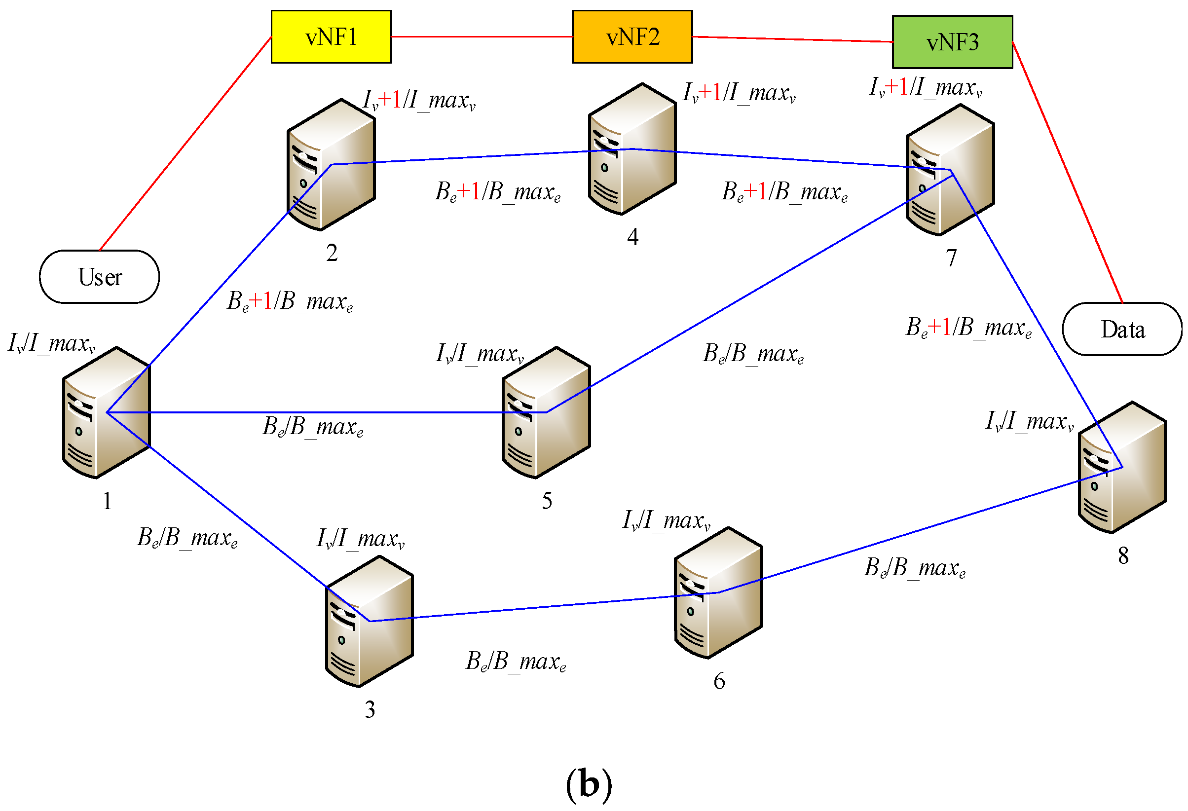
We depict the dynamic SFC deployment and revocation process in Figure 1. At each moment, the situations represented by Figure 1a,b may occur in the network.

In Figure 1a, after the SFC is generated for a request, the SFC will be deployed to the corresponding path when sufficient resources are available. The path’s bandwidth resources will be consumed, assuming a unit is consumed. The IT resources of the server deploying VNF will also be consumed, assuming a unit is consumed, but the user access node and the data provider node do not consume IT resources.

In Figure 1b, after the service time of an SFC expires, the SFC will be dropped from the network. The path’s bandwidth resources and the IT resources of the server that deployed the VNF will also be recovered, if they used units.

To maximize profits, service providers should first attempt make the SFC shorter while meeting the demand. For the overall network, IT resources and bandwidth resources must be balanced properly, which means that SFCs should be distributed as widely as possible, rather than crowding them together, which can create problems. In this way, at any given time, we will have more nodes and paths to choose from to form new SFCs.

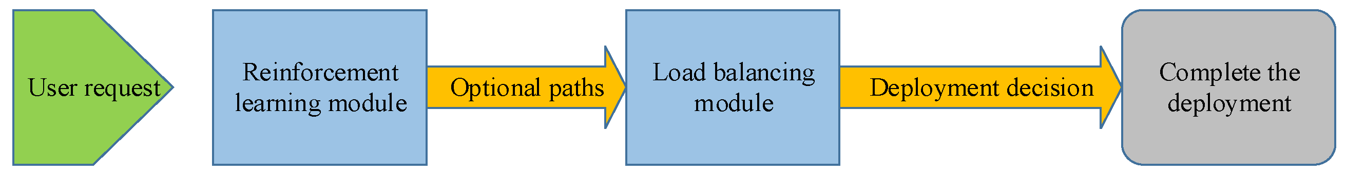
4. Q-Learning Framework Hybrid Module Algorithm

In this section, we use the Q-learning framework hybrid module algorithm (QLFHM) to address dynamic SFC deployment. First, to reduce the problem complexity, we divide the solution process into two parts: we use the RL module to output several of the shortest paths that meet certain requirements. The load balancing module obtains multiple routing outputs from the previous module and finally obtains the solution of the problem. The goal of hierarchical processing is to reduce the training and learning times and achieve an efficient output scheme. The architecture of QLFHM is shown in Figure 2.

4.1. Preliminaries

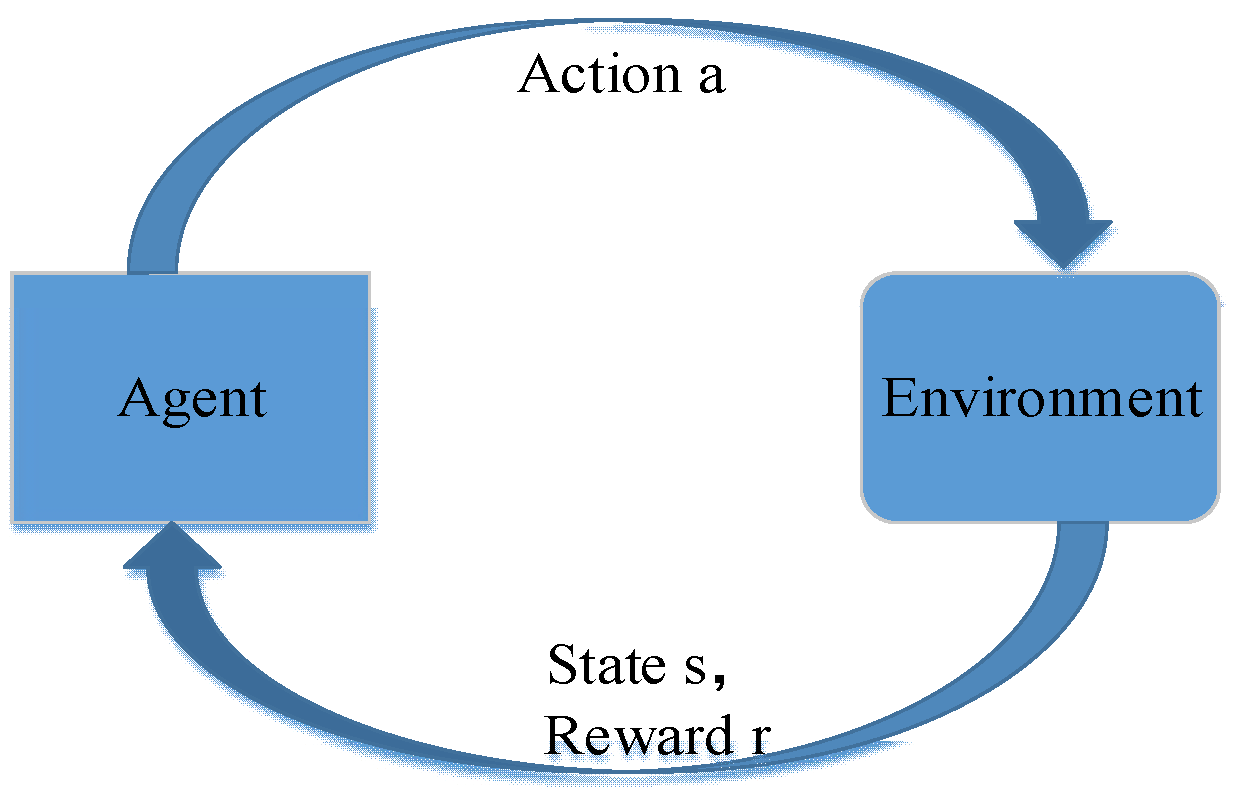
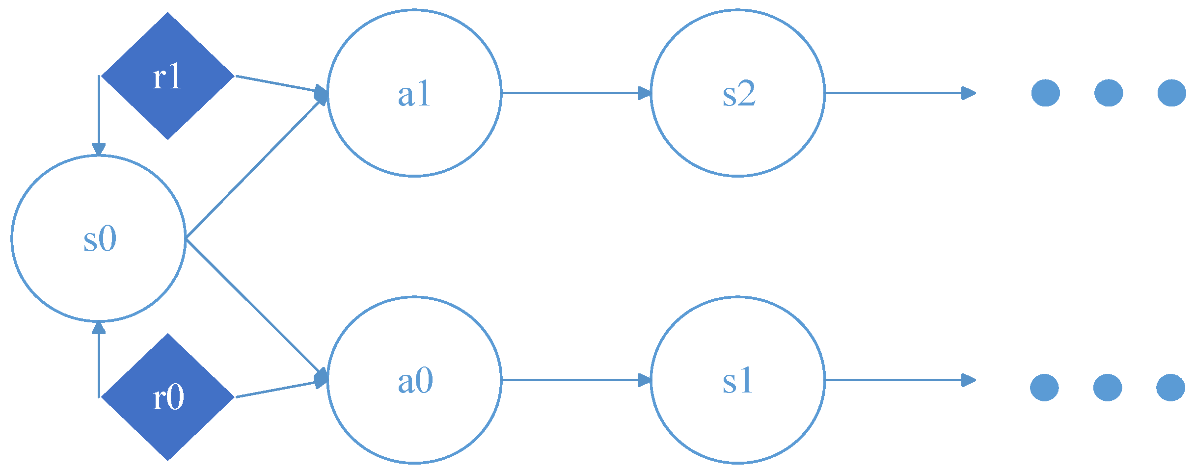
Problems that can be solved by Q learning generally conform to the Markov decision-making process (MDP) and have no aftereffect. That is to say, the next state of the system is only related to the current state information and is unrelated to the earlier state. Unlike the Markov chain and Markov models, the MDP considers actions, that is, the next state of the system is related not only to the current state, but also to the current action taken. The dynamic process of MDP is shown in Figure 3:

The return value r is based on state s and action a, each combination of s and a has its own value of return, then MDP can also be represented as the following Figure 4:

In relation to the problem in this paper, it conforms to the Markov decision making process, but the difference is that the times of decision making for the problem in this paper is limited. Therefore, after our study, we combine the Q-learning with this problem and optimize the Q-learning algorithm for this problem. In this way, we can not only take advantage of the reinforcement learning, but also avoid its defects, which can provide new ideas for dynamic SFC deployment.

A key point of the algorithm proposed in this paper is that it improves the $Q$ matrix and changes the original two-dimensional matrix into a five-dimensional matrix. The five subscripts are $now\_h$, $now\_node$, $action\_node$, $end\_node$, $h$. The subscript $now\_h$ refers to the number of hops that have been visited in the current state; $now\_node$ is the node in which the agent is in the current state; $action\_node$ is the next available node set; $end\_node$ is the node that this SFC will eventually reach; and $h$ is the minimum number of hops that can meet the deployment requirements.

As shown in Figure 5, after the agent responds to the environmental state, the environmental state changes and returns r. The $Q$ matrix is updated with r. The agent will repeat the above behavior until the $Q$ matrix converges. The Q-learning algorithm is shown in Equation (11):

$$Q\left(s,a\right)=Q\left(s,a\right)+\alpha \left(r+\gamma \underset{a^{\prime }}{max}Q\left(s^{\prime },a^{\prime }\right)-Q\left(s,a\right)\right).$$

(11)

The values stored in $Q$ are the recommended values for the next action in each state. The higher a recommended value is, the more it is worth performing. The recommended values are formed during the training phase of the $Q$ matrix.

In Equation (11), $Q$ is a matrix that stores the recommended values of the executable actions in the current state. Depending on these values, the agent can decide which action to take next. In the $Q$ matrix, the subscript $s$ refers to the state, $a$ to the action, $s\prime$ to the future state, $a\prime$ to the future action, and $r$ is the reward value, which comes from the reward matrix $R$. Here, $\alpha$ and $\gamma$ are the studied ratio between 0 and 1.

In $R$, we set the value of the element to 1000, which has same $now\_node$ and $end\_node$ in the subscript. This value represents the reward given when completing the pathfinding task.

For $Q \left[now\_h, now\_node, action\_node, end\_node, h\right]$, Specifically, when the four subscripts $now\_h$, $now\_node$, $end\_node$, and $h$, which represent states, are determined, the subscripts of $action\_node$ are iterated. The maximum value is selected and its subscript $action\_node$ is executed. The advantages of this approach are that (1) it makes the state more observable, and (2) it divides the states into several independent parts that are conducive to parallel programming techniques.

The recommended values stored in $Q$ are determined by Equation (11), which is a simplified version of Equation (12).

$$Q\left(s,a\right)=\alpha \left(r+\underset{a^{\prime }}{max}Q\left(s^{\prime },a^{\prime }\right)\right).$$

(12)

Some of the parameters and variables used in the QLFHM algorithm are described in

Table 1. Parameters and variables in the Q-learning Framework Hybrid Module algorithm (QLFHM) algorithm.

Parameters and Variables	Definition
$G$	Information about network topology
$V$	A list of nodes in a network topology
$V_i$	Node adjacent to node $i$
$h_{max}$	The maximum number of hops allowed by the model
$h_{min}$	The minimum number of hops allowed by the model
$Q$	A 5-dimensional matrix with 5 subscripts {$now\_h$, $now\_node$, $action\_node$, $end\_node$, $h$} that store recommended action values
$R$	A 5-dimensional matrix with 5 subscripts {$now\_h$, $now\_node$, $action\_node$, $end\_node$, $h$} that store action reward values
$h$	The number of hops in the current state
$RE$	User request list, including start and stop nodes, VNF requirements, arrival time, and request online duration
$PA$	Path list that matches the start and stop nodes
$CA$	Path list that satisfies the start and stop nodes and the VNFs requirements
$ONL$	The online SFC list

:

4.2. Reinforcement Learning Module

In this section, we propose the RL module, which is responsible for outputting alternative paths based on the network topology. The content is divided into two parts: a training stage and a decision stage. In the first part, we first provide the original Q-learning training algorithm and then provide the optimized training algorithm for this problem. Both algorithms have advantages and disadvantages. In the second part, we will propose the algorithm used in the decision stage.

4.2.1. Original Q-Learning Training Algorithm

In the training phase, training data are not required; this phase automatically generates the RL model according to the basic network topology information.

Algorithm 1 adopts the standard Q-learning training method, that is, iterative trial and error. The rewards attained during the repeated attempts finally cause the $Q$ matrix to converge. The variable u is added for the greedy algorithm that enables the agent to improve the explored path in most cases, while making it possible to explore new paths.

Algorithm 1. Original Q-learning Training Algorithm

1: initialize the $Q$ matrix with all zero elements; 2: initialize the $R$ matrix; 3: initialize $h_{min}$ and $h_{max}$; 4: $h$ = 0; 5: While True do 6:  randomly generate $v1\in V$;//as the $now\_node$ 7:  randomly generate $v3\in V$;//as the $end\_node$ 8:  For $h< h_{max}$ do: 9:   randomly generate $u\in \left[0,1\right]$; 10:   If $u\le 0.8$ then: 11:    choose the $v2\in V_{v1}$ with the maximum recommended value from $Q$; 12:   End If 13:   If $u>0.8$ then: 14:    randomly choose a $v2\in V_{v1}$; 15:   End If 16:   $v1=v2$; 17:   If $v2=v3$ then: 18:    Write the link to the $Q$ matrix using Equation (12); 19:    Break; 20:   End If 21:   $h$++; 22:   If $h=h_{max}$ then: 23:    Break; 24:   End If 25:  End For 26:  If the $Q$ matrix has basically converged, then: 27:   Break;//return the $Q$ matrix that can be used 28:  End If 29: End While

The advantages of using the Q-learning algorithm in this paper are as follows: (1) we can observe and understand the decision-making process, and the use of the $Q$ matrix is more intuitive and comprehensible; (2) we can quickly convert this algorithm to a deep Q-learning algorithm, which uses a neural network (DQN) to replace the $Q$ matrix for decision making; and (3) Q-learning is conducive to the improvement of the algorithm proposed in this paper and is suitable for solving the problems in this paper.

The algorithm based on Q-learning obtained satisfactory results, but it also faces some problems. For example, in the face of complex situations or too-large networks, the training period will be excessive. Consequently, an improved version is presented in Algorithm 2, which is optimized for our problem.

4.2.2. Optimized Q-Learning Training Algorithm

Algorithm 2 is an improved version of the Q-learning algorithm based on our problem. It abandons the trial-and-error learning mode of the original algorithm and adopts a method similar to neural diffusion, which results in a hundredfold reduction in training time.

In the $Q$ matrix, we did not list the state with one index as in the original algorithm of Q-learning; instead, we divided the state into four indexes. The advantages of this approach are as follows: Algorithm 2 normally executes on a single computer; however, when greater efficiency is required, the algorithm can begin working in a distributed operation starting on line 5. Because the four indexes make some states independent, we can use distributed computing to reduce the execution time. And the main functions in Algorithm 2 are described in Algorithm 3.

Algorithm 2. Optimized Q-learning Training Algorithm

1: initialize the $Q$ matrix with all zero elements; 2: initialize the $R$ matrix; 3: initialize $h_{min}$ and $h_{max}$; 4: $h$ = 0; 5: For each node v ∈ V  do //as the$end\_node$ 6:  $chain$ = [$v$] 7:  Find_way ($Q$, $R$, $G$, $h_{min}$, $h_{max}$, $h$, $chain$) 8: End For

Algorithm 3. Find_way (Q, R, G, hmin, hmax, h, chain)

1: $v0$ = $chain$ [0]; 2: $h$ = $h$ ++; 3: $chain\_tmp$ = $chain$; 4: While $h$ ≤ $h_{max}$ do 5:  For each node $v2 \in V_{v0}$ do 6:   If $v2$ is not in $chain\_tmp$ then 7:    $chain\_tmp$ = $v2$ + $chain\_tmp$; 8:    Find_way ($Q$, $R$, $G$, $h_{min}$, $h_{max}$, $h$, $chain$); 9:    If $h$ ≥ $h_{min}$ then 10:     For $i$ in $chain\_tmp$ do 11: Write the link to the $Q$ matrix, 12: $\mathrm{Q}\left({\mathrm{s}}_i,{\mathrm{a}}_i\right)=0.8\left(r+\underset{a_i{}^{\prime }}{max}Q\left(s_i{}^{\prime },a_i{}^{\prime }\right)\right)$ 13:     End For 14:    End If 15:   End If 16:  End For 17: End While

4.2.3. Complexity Analysis of Original and Optimized Q-Learning Training Algorithm

In this section, we give the time complexity of the original and optimized Q-learning training algorithm.

We use $ite$ to represent the number of iterations of the original Q-learning training algorithm in the trial and error training process, which is a very large number and also the reason for the long training time.

The time complexity of original Q-learning training algorithm is

$$\mathrm{T}=O\left(ite\ast h_{max}\right).$$

(13)

And the time complexity of optimized Q-learning training algorithm is

$$\mathrm{T}=O\left(n^{h_{max}}\right).$$

(14)

where $h_{max}$ is less than 13; and $n$ represents the number of nodes in the topology.

However, $ite$ is not a constant, which will increase significantly with the increase of $n$ and $h_{max}$. And Equation (14) shows the worst case of a full-connected-network. Therefore, for the problem solved in this paper, the optimized algorithm will consume much less time.

4.2.4. Q-Learning Decision Algorithm

After the $Q$ matrix has largely converged, the training phase terminates. During the decision phase, we use the $Q$ matrix to output multiple alternative paths $CA$ that meet the input requirements. These paths are then sent to the load balancing module, which makes a final selection. The whole process is described in Algorithm 4.

Algorithm 4. Q-learning decision-making process

1: read the trained matrix $Q$ 2: read the user request list $RE$ 3: For every $re$ in $RE$ do 4:  Select some optional paths $PA$ from $Q$; 5:  For every $pa$ in $PA$ do 6:   If the $pa$ can deploy the required VNFs then 7:    add $pa$ to the candidate list $CA$; 8:   End If 9:  End For 10:  If the candidate list $CA$ is empty then 11:   deployment for this $re$ failed; 12:   continue; 13:  End If 14:  Send the candidate list $CA$ to the load balancing module; 15: End For

It is worth mentioning that even in the decision stage, the $Q$ matrix is not necessarily permanently static; it can be adjusted based on the actual situation to support supplementary learning for new paths or nodes or the removal of expired paths and nodes.

4.3. Load Balancing Module

The load balancing module adopts a scoring system. It scores each SFC output from the previous module, and the optimal choice will be deployed.

First, consider the link weight $weigh{t}_{link}\in \left[0,1\right]$ and the node $weigh{t}_{node}\in \left[0,1\right]$, which represent a proportion that focuses on the link or node. When no special requirement exists, we set the weights to 0.5, 0.5:

$$weigh{t}_{node}+ weigh{t}_{link}=1.$$

(15)

Next, we consider the weights of specific nodes $weigh{t}_{node v }\in N$ and specific links $weigh{t}_{link e }\in \mathrm{N}$ is considered. To urge the SFC to go through a node or link, we increase its weight, which increases the probability that the SFC will traverse that node or link. When no special requirement exists, the weights remain unchanged.

Finally, the link bandwidth resources $B_e$ and node computing resources $I_v$ are combined with the weights mentioned above to obtain the final score. The higher the score is, the more the path represented is worth deploying. The score is calculated by Equation (16):

$$score= weigh{t}_{link}\ast [\sum _{e\in SFC}(weigh{t}_{link e }\ast B_e)]+weigh{t}_{node}\ast [\sum _{v\in SFC}(weigh{t}_{node v }\ast I_v)].$$

(16)

Using Equation (16), we can construct Algorithm 5, which takes the output of the RL module as input and outputs the final decision results.

Algorithm 5. The load balancing scoring process

1: read the information from $G$ 2: read the candidate list $CA$ 3: For every $pa$ in $CA$ do 4:  calculate the score of $pa$ using Equation (15); 5: End For 6: take the path with the highest score from the candidate list $CA$; 7: record the start time $t_{start-re}$, and record the end time $t_{end-re}$ 8: add $re$ to the online SFC list $ONL$; 9: change the resource residuals in the topology; 10: If any $re$ in $ONL$ reaches $t_{end-re}$ then 11:  return the related resources in the topology; 12: End If

Due to the flexibility of the independent scoring system, it can be customized for problems that involve required traversal nodes as well as nodes that need to be bypassed. By further adjusting parameters and structures, this algorithm can also be used to solve the problems related to virtual machine consolidation and dynamic application sizing [37].

Dividing the SFC dynamic network deployment problem into two parts reduces the scale of the problem and improves the execution efficiency. First, the improved Q-learning training algorithm results in a training time that is one hundred times smaller. In addition, the independent scoring system is highly flexible and can be customized for specific problems.

5. Performance Evaluation and Discussion

In this section, we compare the QLFHM algorithm with two other algorithms to evaluate the performance of the proposed dynamic SFC deployment method. We first describe the simulation environment and then provide several performance metrics used for comparisons in the simulation. Finally, we describe the main simulation results.

5.1. Simulation Environment

The simulation uses the US network topology, which has 24 nodes and 43 edges. Here, we assume that the server and switch are combined, which means that all nodes have local servers but not necessarily all VNFs. The server’s IT resource capacity is 4 units, and the bandwidth capacity of each physical link is 3 units. Note that each VNF occupies 1 unit of IT resources, and each traversed link occupies only 1 unit of bandwidth resources. The online time of each request follows a uniform distribution, and the arrival time is subject to a Poisson distribution.

Some servers can support 5 VNF types, but not all servers support all VNF types. For each VNF type, the IT resources of each VNF consume one unit, and each unit can serve one user. Assume that the number of VNFs per user requested in SFC is normally distributed from [2,3,4]. To compare the proposed algorithm with existing algorithms, we implement the algorithm in [14], which has a high success rate due to its use of ILP. Although the algorithm is optimized for time, it still requires considerable time; thus, it is not shown on the time comparison graph. We also implement the algorithm in [28], which has good execution efficiency.

5.2. Performance Metrics

We used the following metrics in the simulation to evaluate the performance of our proposed algorithm. For the dynamic network with limited resources, we selected three sets of data for analysis: the request acceptance ratio, the average service provider profit, and the calculation time per request.

(1) Request acceptance ratio: This value is the ratio of incoming service requests that have been successfully deployed on the network to all incoming request. Ratio $A$ is defined as

$$A= \frac{Numbe{r}_{successfully deployed SFC}}{Numbe{r}_{input service requests}}.$$

(17)

(2) Average service provider profit: This value is the total profit earned by the service provider after processing the input service requests. The average service provider profit K can be calculated as follows:

$$K = \sum _{i\in RE}\left(\frac{3}{2}\ast num\_vnf{s}_i-l_i \right) \ast \omega \ast y_i.$$

(18)

(3) Calculation time per request: This value reflects the decision time required before each SFC is deployed. The calculation time per request $C$ is expressed as follows:

$$C= \frac{Total running time}{Numbe{r}_{input service requests}}.$$

(19)

5.3. Simulation Results and Analysis

We divide the experiment into two parts and present and analyze the results separately.

The first part involves comparing and analyzing the performances of the QLFHM algorithm and the other two selected benchmark algorithms in the simulated network. The second part compares and discusses some parameters that can affect the performance of the QLFHM algorithm and demonstrate its flexibility and modular capabilities.

We obtained each data point by averaging the results of multiple simulations. We executed the simulations on an Ubuntu virtual machine running on a computer with a 3.7 GHz Intel Core i3-4170 and 4 GB of RAM. The algorithm models were coded in Python.

5.3.1. Performance Comparison in a Dynamic Network

This section provides comparison results from simulating the algorithm proposed in this paper and the two other selected algorithms [14,28] on an SFC dynamic deployment problem. Three sets of data were selected for analysis: the request acceptance ratio, service provider average profit, and the calculation time required for each request.

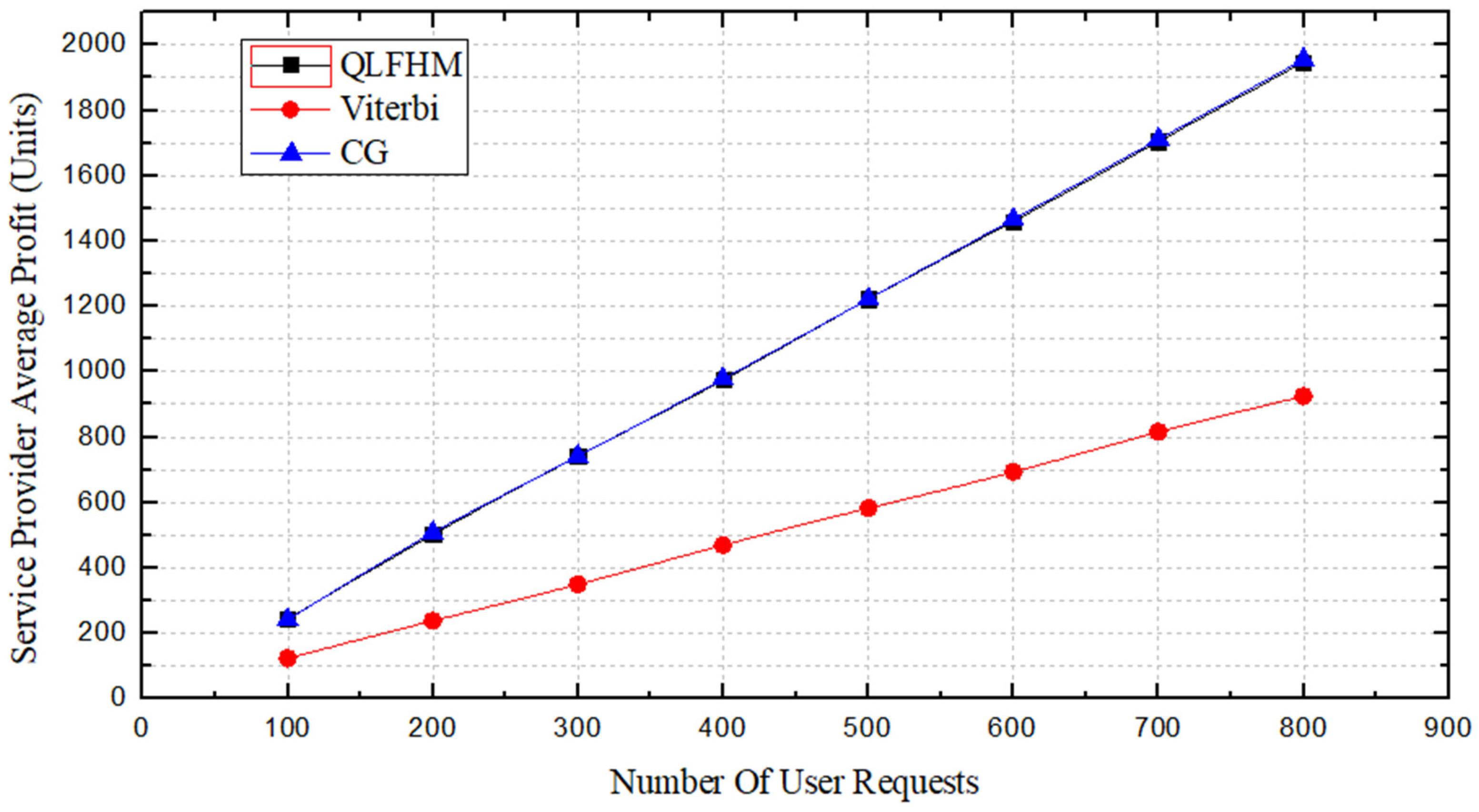
Figure 6 shows a comparison of the request acceptance ratio achieved by the three algorithms. As Figure 4 shows, when the number of requests is less than 400, the request acceptance ratio is unstable due to insufficient data. However, the QLFHM and CG algorithms always achieve better results than does the Viterbi algorithm. The request acceptance ratio of the CG algorithm is slightly different because more than one optimal path exists in some cases, and the two algorithms use different path selection strategies. After the algorithms select different paths, the overall situation will also differ, resulting in some overall differences. After the number of requests exceeds 400, the request acceptance ratio of the three algorithms tends to become stable; at that point, the request acceptance ratio of the QLFHM algorithm is roughly the same as that of the CG algorithm using ILP. This result demonstrates that the deployment success ratio of the QLFHM algorithm is higher than that of the Viterbi algorithm and is close to the optimal solution at any request scale.

Figure 7 shows a comparison of the profits of the service providers achieved by the three algorithms. There is almost no profit difference between the QLFHM and CG algorithms. However, as the number of requests increases, the profit difference between the QLFHM algorithm and the Viterbi algorithm gradually increases. Because the CG algorithm uses ILP, its deployment scheme is close to optimal. The QLFHM algorithm obtains results not much different from CG, indicating that the deployment scheme of the QLFHM algorithm is close to optimal. We are confident that under larger numbers of requests, the profit obtained using the QLFHM algorithm will never be less than that obtained by the other two algorithms.

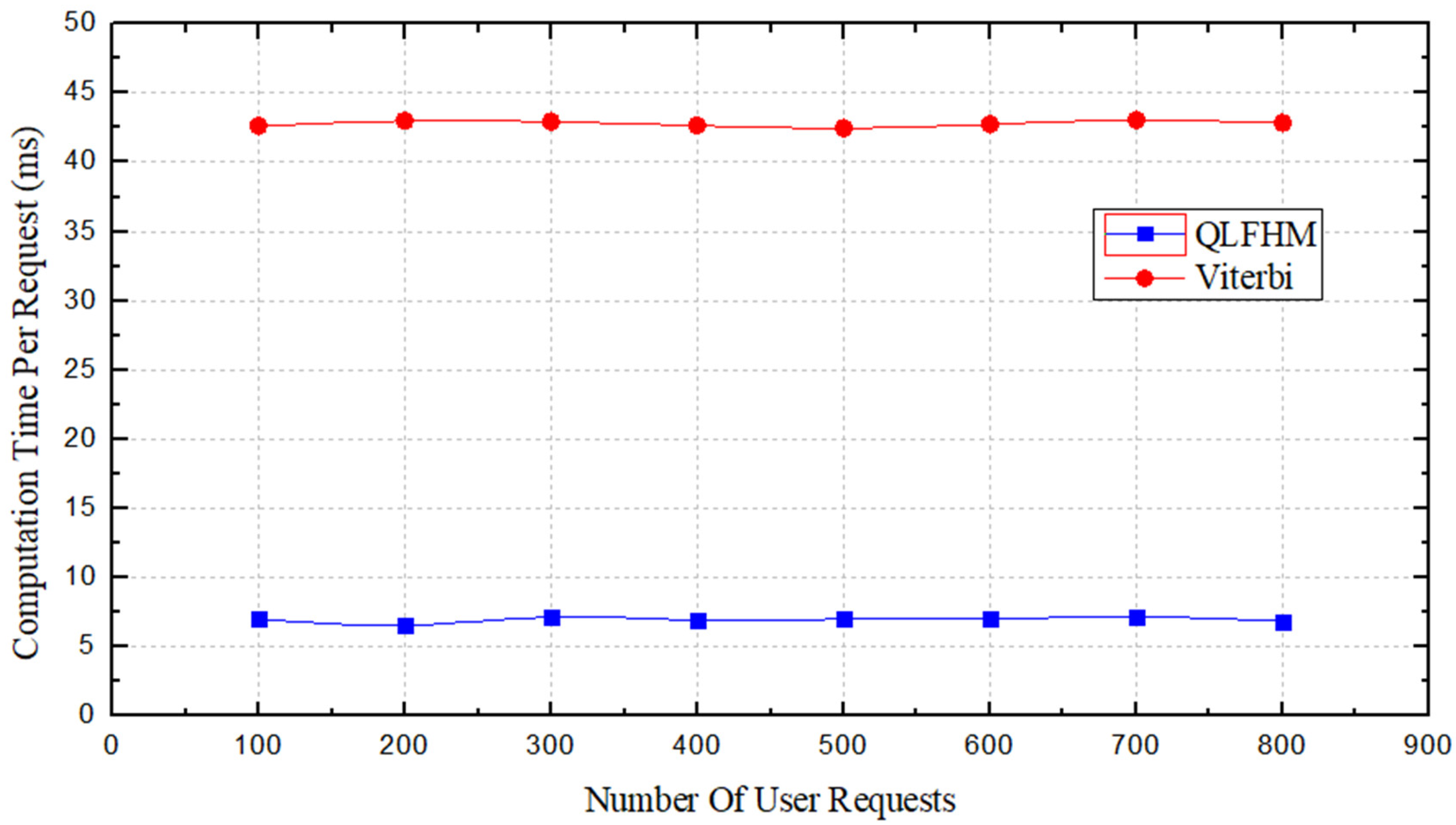
In Figure 8, we compare the average operation time of only two algorithms. We know from [14] that the operation time of the CG algorithm is much longer than that of the other two; therefore, the CG algorithm’s performances are not included in the figure. Figure 8 shows that the average operation time of the QLFHM algorithm is approximately 6 times less than that of the Viterbi algorithm. This result indicates that among the three algorithms, the QLFHM algorithm yields the fastest result.

By comparison, we can draw the following conclusion. Under the condition that the output deployment scheme is close to the optimal solution, the Q algorithm provides a result faster than does the general heuristic algorithm. The request acceptance ratio and the service provider average profit values indicate that the algorithm considers the global network insofar as possible—that is, it better guarantees the load balance.

5.3.2. Effects of the Use Ratio $\lambda$

We know that the $Q$ matrix stores several link strategies between any two points in the topology. However, in the actual output process, scoring all the links may not be the best option. Here, we test the proportion of the use of the RL output, which we call the use ratio $\lambda$.

There are three parameters $x1$, $x2$, $x3$ associated with $\lambda$ in step 4 of Algorithm 4. The parameter $x1$ represents the ratio of the recommended value of the next action in a state. For example, if $x1$ is set to 0.6, alternative paths can be added if their recommended value is greater than 0.6 multiplied by the maximum recommended value. The parameter $x2$ limits the number of paths to find. For example, when $x2$ is set to 100, the algorithm will stop looking after finding 100 candidate paths. The parameter $x3$ represents the longest length of a single path, depending on the number of VNFs required.

To perform a comparison, we divide $\lambda$ into three scenarios: low $\lambda$, balanced $\lambda$ and high $\lambda$. The use ratio design is listed in

Table 2. The design of the use ratio $\lambda$ .

Use Ratio	${\mathit{\lambda }}_{\mathit{l}\mathit{o}\mathit{w}}$	${\mathit{\lambda }}_{\mathit{b}\mathit{a}\mathit{l}\mathit{a}\mathit{n}\mathit{c}\mathit{e}\mathit{d}}$	${\mathit{\lambda }}_{\mathit{h}\mathit{i}\mathit{g}\mathit{h}}$
$x1$	0.79	0.6	0.4
$x2$	100	100	100
$x3$	7	7	7

.

After completing this analysis, we selected the balanced parameter (which is the $\lambda$ parameter used in the previous section). We used the same three metrics (request acceptance ratio, service provider average profit, and computation time per request) for analysis.

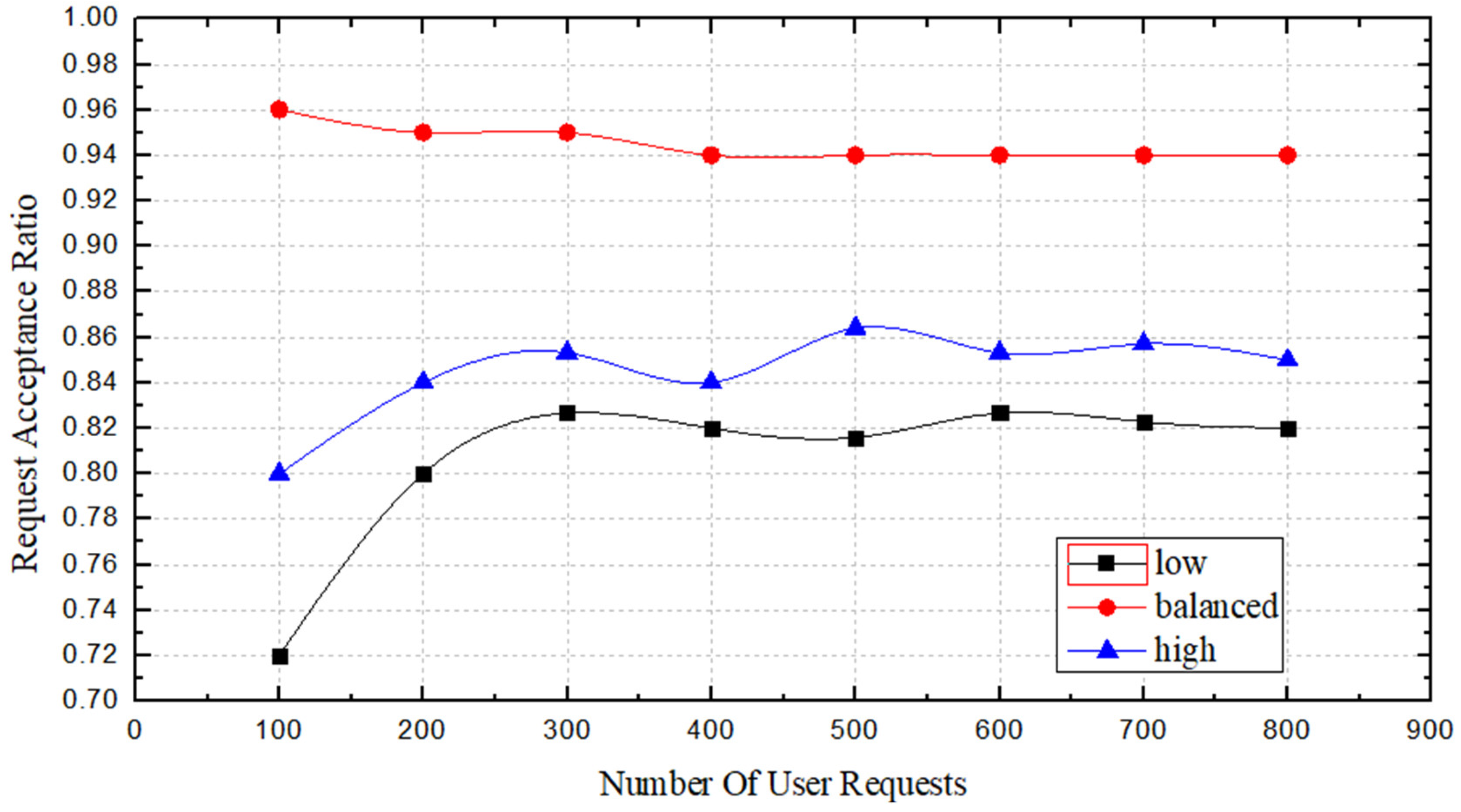
From Figure 9, we can see the acceptance ratio for requests in the three $\lambda$ states. When the number of requests is less than 400, the acceptance ratio of the three $\lambda$ states is not particularly stable; of these, the fluctuations of ${\lambda }_{high}$ and ${\lambda }_{low}$ are high, while the fluctuation of ${\lambda }_{balanced}$ is much higher than the other two $\lambda$ states. When the request number is greater than 400, the acceptance ratio of all three $\lambda$ states tends to be stable, but the acceptance ratio of ${\lambda }_{balanced}$ is approximately 10% higher than those of the other two states. This is because when the $\lambda$ state is ${\lambda }_{high}$, some longer paths may obtain high scores; thus, they will be selected for deployment, occupy more bandwidth resources, and affect other SFC deployments. When the $\lambda$ state is ${\lambda }_{low}$, the number of options for participation is insufficient, and the optimal choice cannot be found.

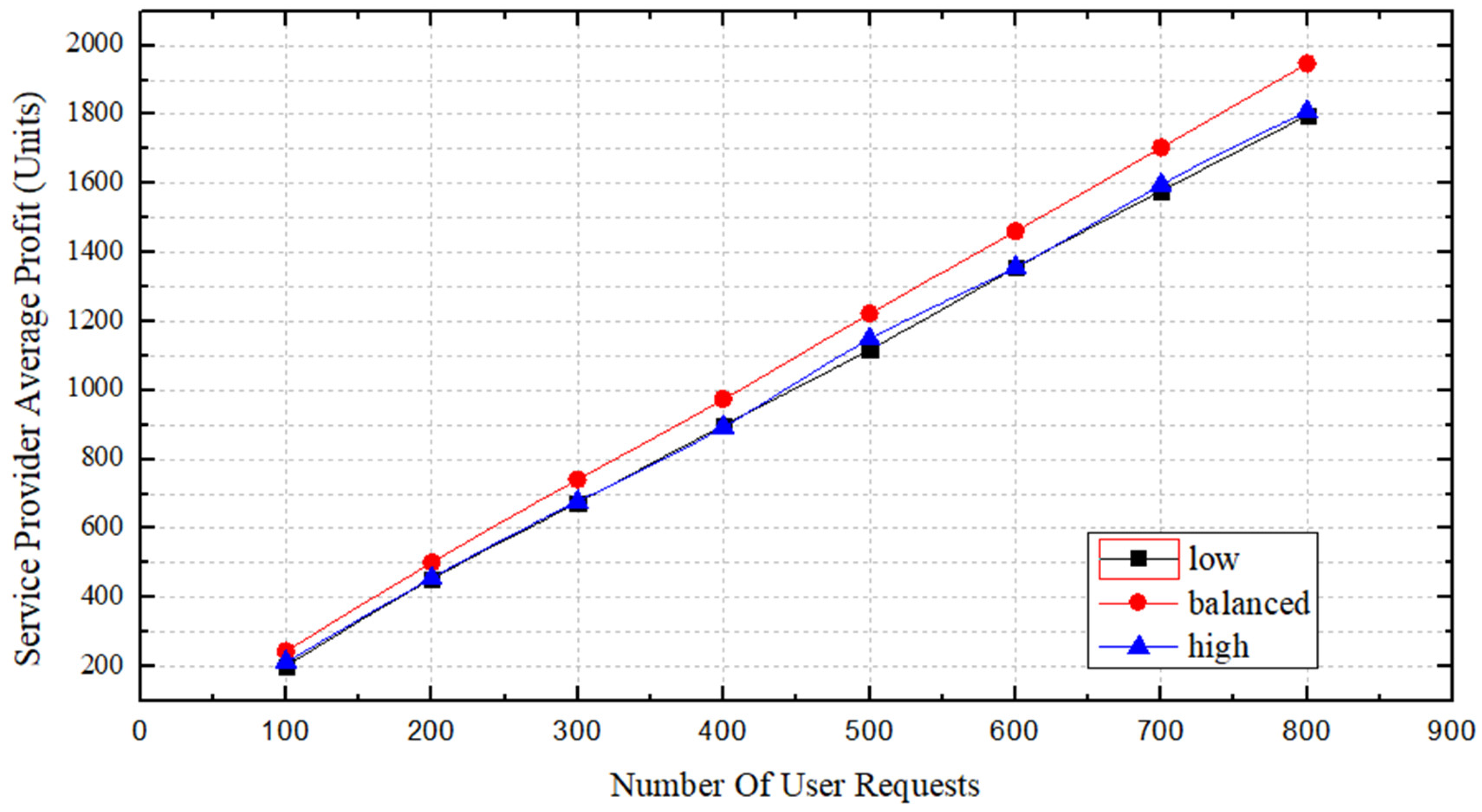
In Figure 10, we compare the service provider’s profits in the three $\lambda$ states. The profit difference among the three states is not obvious when the number of requests is low; however, as the number of requests increases, the profit margins in the ${\lambda }_{high}$ and ${\lambda }_{low}$ states remain close and their slopes are approximately the same. In contrast, the profit of ${\lambda }_{balanced}$ increases at a greater slope, increasing the gap between its profits and those of the other $\lambda$ states. This result is related to the deployment success rate and the length of the deployed SFCs. We are confident that when the $\lambda$ state is ${\lambda }_{balanced}$, the profit obtained by using this algorithm will be larger than the profits obtainable using the other two states of $\lambda$.

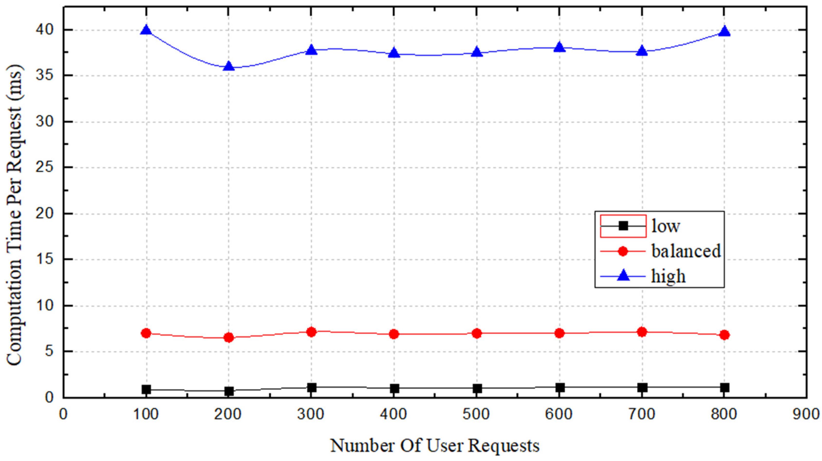
Figure 11 shows a comparison of operation times under the three $\lambda$ states. The average operation time in the ${\lambda }_{low}$ and ${\lambda }_{balanced}$ states is largely stable, while some fluctuation occurs in the ${\lambda }_{high}$ state. The value of $\lambda$ determines the number of candidate paths that participate in the score stage; consequently, the operation time is proportional to the value of $\lambda$. However, as shown, we found that the average operation time of the ${\lambda }_{balanced}$ value is closer to the ${\lambda }_{low}$ state and better matches the desired time efficiency.

After conducting this comparison, we think that the ${\lambda }_{balanced}$ setting is better than the ${\lambda }_{high}$ or ${\lambda }_{low}$ settings. These results suggest that in some cases, the local optimum is not the global optimum. On one hand, the ${\lambda }_{balanced}$ setting helps to reduce the output time. On the other hand, it can reduce the operational overhead of the service provider. Overall, the setting represents a tradeoff between reducing execution time and achieving an optimal solution.

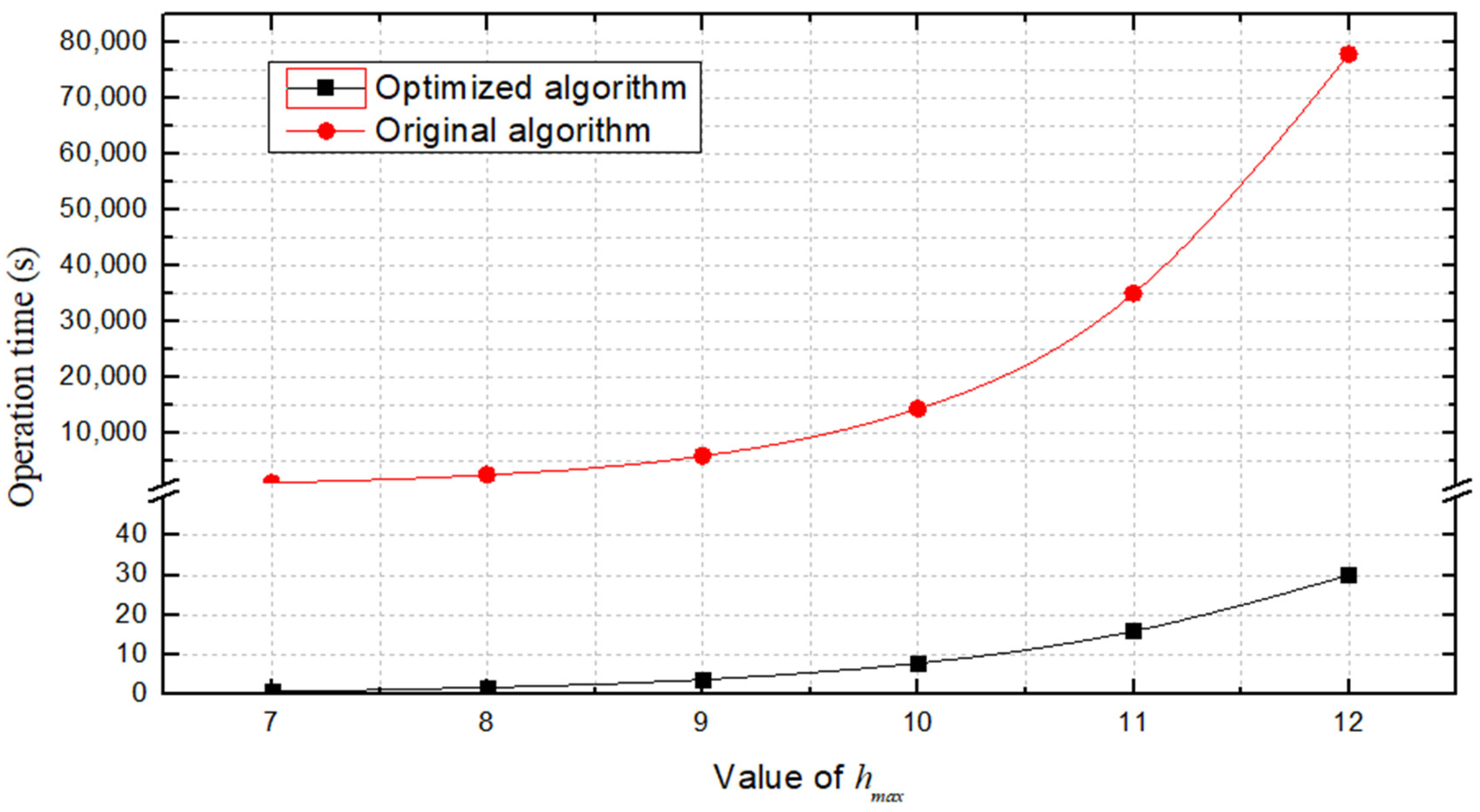
5.3.3. Comparison of Training Time

In this sub-section, we show a comparison of operation time between original and optimized Q-learning training algorithm. We change $h_{max}$ to make the path we need to find longer, and the number of paths increases, which is the same as the case when the network topology keeps getting bigger. Taking the convergence of $Q$ matrix as the termination time, the comparison results are shown in Figure 12.

From Figure 12 we can see that the operation time is not at an order of magnitude, and the gap grows larger and larger with the increase of $h_{max}$. This is because the times of trial and error training iterations of the RL is very large. Take $h_{max}$ as 7 for example, there are 10,000 iterations in 5 s, and 2,252,000 iterations are needed to make the $Q$ matrix to converge. When $h_{max}$ is larger, it is more difficult to achieve the convergence of $Q$ matrix.

From the comparison results, it can be seen that in any practical situation, the optimized algorithm can produce a convergent $Q$ matrix within 1 min. This not only solves the problem of reducing the training time, but also solves the problem of judging whether the $Q$ matrix converges.

The entire simulation comparison shows that compared with the benchmark algorithms, the QLFHM algorithm proposed in this paper has excellent performance and can make decisions based on requests in a very short time while maximizing the service provider’s profits. Moreover, the three adjustable parameters not only increase the algorithm’s flexibility but also leave room for improvement.

6. Conclusions

This study investigated SFC deployment in a dynamic network. We designed an effective algorithm (QLFHM) to solve this problem. In the QLFHM algorithm, we consider the network load balance and make corresponding countermeasures to reflect the real-time changes in a dynamic network. The algorithm first reads the network topology information and then learns the topology routing scheme through the RL module. Then, it uses the load balancing module to select the optimal solution from several candidate schemes output by the RL module. The improved learning algorithm improves the efficiency of addressing this specific type of problem; it not only capitalizes on the decision-making advantages of RL but also avoids a lengthy training process. Finally, we conducted extensive simulation experiments in a simulated network environment to evaluate the performance of our proposed algorithm. The experimental results show that the performance of the proposed QLFHM algorithm is superior to that of the benchmark algorithms CG and Viterbi when processing service requests. We are confident that while QLFHM algorithm ensures the security of user data, its performance advantages are reflected by the decision time, load balancing, deployment success rate and deployment profit when deploying SFCs.

In future work, we will further carry out other related researches such as the migration of virtual machines for the deployed VNFs [38], the energy-saving operation of servers in the network [39], and the decentralization of resource allocation controllers [40] to extend our current study.