Abstract
Because of the cyclic symmetric structure of rolling bearings, its vibration signals are regular when the rolling bearing is working in a normal state. But when the rolling bearing fails, whether the outer race fault or the inner race fault, the symmetry of the rolling bearing is broken and the fault destroys the rolling bearing’s stable working state. Whenever the bearing passes through the fault point, it will send out vibration signals representing the fault characteristics. These signals are often non-linear, non-stationary, and full of Gaussian noise which are quite different from normal signals. According to this, the sub-modal obtained by empirical wavelet transform (EWT), secondary decomposition is tested by the Gaussian distribution hypothesis test. It is regarded that sub-modal following Gaussian distribution is Gaussian noise which is filtered during signal reconstruction. Then by taking advantage of the ambiguity function superiority in non-stationary signal processing and combining correlation coefficient, an ambiguity correlation classifier is constructed. After training, the classifier can recognize vibration signals of rolling bearings under different working conditions, so that the purpose of identifying rolling bearing faults can be achieved. Finally, the method effect was verified by experiments.
1. Introduction
Rolling bearings are widely applied in rotating parts of various mechanical equipment, often as core components. Its fault will cause very serious consequences in the entire system. It is very difficult and inefficient to identify faults via disassembling inspection in the event of a fault. The vibration signal of rolling bearing contains a wealth of dynamics characteristics. In particular, corresponding impact signal will show in case of rolling bearing fault [1,2,3]. Therefore, a research hot spot is to identify the working condition of the rolling bearing by analyzing vibrational signal of the rolling bearing, and then identify the fault [4,5,6].
Vibration signals of rolling bearings are generally non-stationary, nonlinear [7,8,9], often in non-Gaussian distribution [10,11]. Meanwhile, there are a large number of noise signals owing to the complex working environment, and these noises are mainly Gaussian noise [12,13]. In view of such characteristics, we need to find an analysis method that can effectively analyze non-stationary nonlinear signals and also overcome Gaussian noise interference. Wavelet transform is a good tool for processing non-stationary signals, and many scholars have studied the failure of rolling bearings by using wavelet transform. Reference [14] mainly studies the fault diagnosis of local defects of rolling bearings based on wavelet feature extraction. In Reference [15], the feature of rolling bearing signals is extracted by using the time bound integral of continuous wavelet transform coefficient. But wavelet decomposition is constrained by wavelet basis functions [14,15,16], and the number of decomposition layers and thresholds of wavelets will affect the noise filtering effect during noise filtering [13,16]. Empirical mode decomposition (EMD) is a very good method for analyzing non-stationary signals, which enjoys many applications in fault diagnosis of rolling bearings [17,18]. However, EMD has problems such as modal mixture and endpoint effects [19,20]. Combining EMD’s adaptability and theoretical framework of wavelet analysis, Gilles proposed a new signal processing method, namely empirical wavelet transform (EMT) [21]. The method adaptively divides the signal frequency spectrum into several frequency bands by extracting maximum value point of the frequency domain, and constructs a suitable orthogonal wavelet filter bank to separate each frequency band. Each separated frequency band corresponds to a signal in the time domain. This signal is referred to as a modal of the original signal. This method avoids the problems of EMD modal in aliasing and endpoint effects, while inheriting the strength of EMD and wavelet analysis methods, thus it is a very good method for processing non-stationary signals.
According to the above analysis, we propose a novel rolling bearing fault diagnosis method based on an empirical wavelet transform (EWT) sub-modal hypothesis test and ambiguity correlation classification. First, rolling bearing vibration signals are subjected to EWT decomposition to obtain each modal. Each modal often still contains very complicated information. To obtain more detailed information, each modal is subjected to secondary EWT decomposition to obtain a sub-modal of each modal. Hypothesis test of Gaussian distribution is performed for all sub-modals one by one, and a sub-modal identified as following Gaussian distribution is regarded as Gaussian noise. All sub-modals following Gaussian distribution, i.e., noise, are deleted to reconstruct the signal. Ambiguity function has the characteristics of high resolution and strong clutter suppression ability, and can deal with non-stationary signals very well. [22] Then, an ambiguity correlation classifier is constructed by taking advantage of ambiguity function and combining correlation coefficients. The ambiguity correlation coefficients of the signals to be identified and three types of known sorting signals (normal signal, outer ring fault signal, inner ring fault signal) are separately calculated. Then, classification of the signals to be identified is provided to achieve the purpose of identifying the working state of the rolling bearing.
Next, we will introduce the implementation process of this method in detail: in Section 2, the basic principles of EWT will be introduced, noise will be filtered, and signals will be reconstructed via the hypothesis test. In Section 3, the basic principles of ambiguity correlation classifier will be introduced. In Section 4, the effectiveness of the method in rolling bearing fault diagnosis will be verified by experiments. Finally, conclusions will be drawn in Section 5.
2. Denoising Method Based on EWT and Hypothesis Test
2.1. Basic Principles of EWT
Gilles. J et al. [23] put forward the EWT method in 2013. The method first assumes that frequency spectrum of the signal is compactly supported into N continuous parts , (, ). Where, indicates boundary between different parts, . The partition graph is a transition section with as the center and as the thickness. After determining the segmentation interval, the method defines band-pass filter on each segmentation interval . According to this concept, Gilles reconstructs the empirical wavelet using the Meyer wavelet reconstruction method. When any n is greater than 0, empirical scale function and empirical wavelet function can be denoted in formulas as follows:
In the formula:
where is width, is related function, is a parameter.
Traditional wavelet transform is adopted to construct EWT by assuming and respectively as Fourier transform and its inverse transform. The high frequency component of empirical wavelet is obtained via inner product of signal and empirical wavelet function, with its mathematical expression shown as follows:
The low-frequency component can be obtained by calculating the inner product of the signal and empirical scale function, with its mathematical expression shown as follows:
The reconstructed original signal is obtained via high-frequency component and low-frequency component, with its mathematical expression shown as follows:
The Fourier transform of and in Equation (8) is and , and then mathematical expression of frequency-amplitude modulation signal is obtained:
The final original signal can be represented by its various modes:
There is a signal expression as follows:
Its waveform is shown in Figure 1.
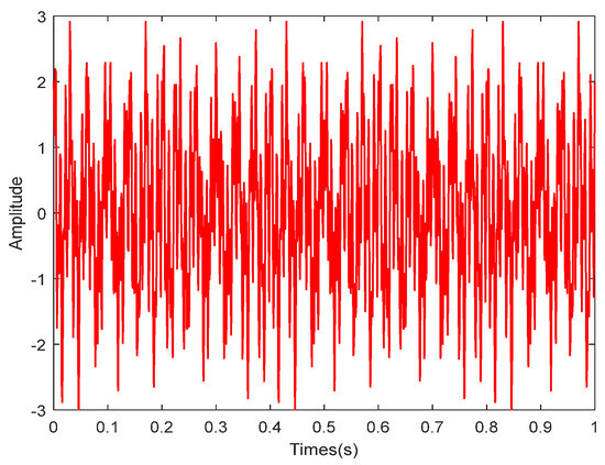
Figure 1.
Signal time domain simulation.
The spectrum of signals is reached by Fourier transform. Then, according to EWT theory, its spectrum is divided, and eight bands are obtained. As shown in Figure 2.
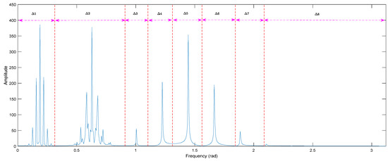
Figure 2.
The spectrum divided by empirical wavelet transform (EWT).
The time domain signal corresponding to each frequency band is a modal of the original signal, that is, the signal has eight modals, . As shown in Figure 3.
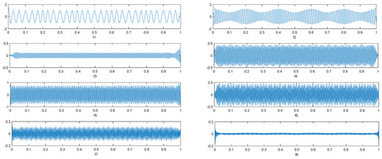
Figure 3.
Decomposition results of signals by EWT.
2.2. Filtering Method Based on EWT Sub-Modal Hypothesis Test
In the frequency spectrum of signal, characteristic of some frequency bands is mainly provided by useful signals, but that of some frequency bands is mainly provided by noise. Empirical wavelet transform divides the frequency spectrum into frequency bands according to the frequency spectrum characteristics of signals. The time domain signal corresponding to each frequency band is a modal of the original signal. Whether a modal follows Gaussian distribution is judged from hypothesis test of Gaussian distribution of each modal. If yes, the modal is considered as Gaussian noise. Useful signal components in rolling bearing vibration signal do not follow Gaussian distribution, while noise follows Gaussian distribution. This method is proposed exactly based on this feature. Under normal circumstances, the modals obtained from EWT decomposition of signals still contain abundant information. To obtain more detailed information, each mode is separately subjected to secondary EWT decomposition to obtain a sub-modal of the modal. The sub-modal is a component with detailed signal. In the hypothesis test of Gaussian distribution of the sub-modal, if it is determined as Gaussian distribution, it can then be determined as Gaussian noise which should be deleted. Afterwards, the signal is reconstructed to obtain a filtered signal. The basic process is shown in Figure 4.
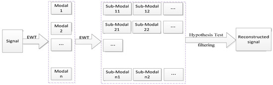
Figure 4.
Filtering process based on the EWT sub-modal hypothesis test.
2.3. Simulation Experiment
Effectiveness of the method in Gaussian noise filtering is verified by simulation signals. Simulation signal is set as . Where, , as shown in Formula (12), is a pollution-free signal. To avoid generality loss, is assumed as mixed Gaussian noise, which is a mixture of Gaussian signals with mean and variance of (0, 1), (2, 5), (4, 10). is noise weight. When are respectively [0.01, 0.05, 0.09, 0.18, 0.48], the corresponding signal-to-noise ratios (SNRs) are respectively [13.5392, 5.5804, 0.4700, −5.5456, −14.065].
Let us take , signal-to-noise ratio SNR1 = 13.5392 as an example. The time domain waveforms of the three signals , , are shown in Figure 5, and the frequency spectrum, i.e., frequency domain waveform, is shown in Figure 6.
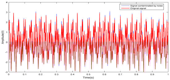
Figure 5.
Signal simulation.
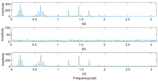
Figure 6.
Frequency of the signals: (a) original signal; (b) noise; (c) contaminated signal.
Signal is subjected to EWT decomposition, with its frequency spectrum divided into 12 continuous frequency bands . As shown in Figure 7 each segment of frequency spectrum corresponds to a modal of the time domain. That is, consists of 12 modals represented as .
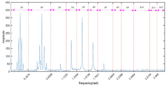
Figure 7.
The spectrum of contaminated signal divided by EWT.
For each modal of , secondary EWT decomposition is performed to obtain sub-modal of each modal. Gaussian distribution hypothesis test with a 95% confidence level is performed for each sub-modal. The test results are shown in Table 1. Where, “1” indicates that the sub-modal satisfies the hypothesis of “not following Gaussian distribution” and needs to be retained; while “0” represents an opposite result, with it identified as noise that needs to be filtered.

Table 1.
Hypothesis test results of sub-modals.
For example, among the four sub-modals of modal F1, the 4th one is judged as satisfying Gaussian distribution and identified as Gaussian noise. Therefore, only the first three modals are summed in F1 reconstruction, and the 4th sub-modal is filtered. Signal can be reconstructed after filtering sub-modal identified as noise. Most of the traditional filtering methods have problems in parameter selection. For example, median filtering needs order setting, moving average filtering needs the setting of the number of moving points, and wavelet filtering needs threshold setting. However, there is no problem of parameter selection in the noise filtering method, and good self-adaptability is demonstrated. The filtering effects obtained by comparing various methods under different signal-to-noise ratios are shown in Table 2.
Table 2.
The filtering results with different signal-to-noise ratios (SNRS).
Table 2 shows that the selection of parameters in different SNRs of the common filtering methods, such as median filter, moving average filter, and wavelet filter, greatly affects the filtering effect. Meanwhile, this scheme based on the EWT sub-modal hypothesis test does not require parameter adjustment, and the filtering effect is obvious in different SNRs.
3. Ambiguity Correlation Classifier
3.1. Ambiguity Correlation Theory
Ambiguity function has the characteristics of high resolution and strong clutter suppression ability, and can deal with non-stationary signals very well. Many scholars have used it to study radar signals [24,25,26]. Correlation coefficient is a good way to measure the similarity of two signals, and it is simple in computation. The combination of these two methods not only reduces calculation amount, but also avoids the interference from cross terms of ambiguity function. With two signals x(t) and y(t), the steps of calculating the ambiguity correlation coefficients between them by using the ambiguity correlation classifier are as follows:
- (1)
- Calculate correlation function of the ambiguity function of the two signals x(t) and y(t)
- (2)
- Calculate the normalized correlation coefficient using correlation function, with mathematical expression shown as follows:
- (3)
- Take the correlation coefficient when τ = 0 or θ = 0
- (4)
- Calculate the ambiguity correlation coefficient
3.2. Basic Principles of Classifiers
Ambiguity correlation classifier belongs to one-to-one classifier.
Firstly, EWT is used to decompose the signal into sub-modes, and the Gaussian distribution hypothesis test was carried out one-by-one for all sub-modals. The sub-modals which are judged to obey Gaussian distribution, namely Gaussian noise, are removed to reconstruct the signal. Then suppose class A signal and class B signal are classified and calculate the ambiguity correlation coefficients of test signal C and class A and class B, respectively. For which ever correlation coefficient is higher, the signal C belongs to that type. The basic process can be represented in Figure 8.
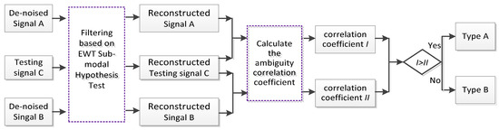
Figure 8.
The basic process of the ambiguity correlation classifier.
4. Experimental Research
Experimental Data Collection
In this paper, the data of Case Western Reserve University was adopted for analysis and collected vibration signals were applied for detection. The test bearing was the drive end bearing of a deep groove ball bearing, model SKF6205. Inner and outer rings of the bearing were locally damaged manually using an electric discharge machine, and piezoelectricity plus a sensor mounted on the upper end of motor output support bearing was used to collect the data. The field acquisition device is shown in Figure 9.
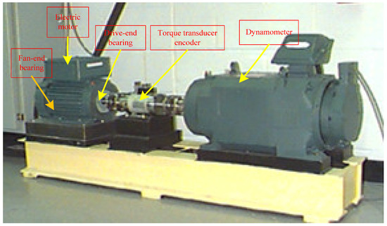
Figure 9.
Test rig and data acquisition equipment.
Bearing speed was 1797 r/min. At 12 kHz sampling frequency, the collected data length N was 3500 points. They were normal signals, outer ring fault signal and inner ring fault signal. Respectively, as shown in Figure 10.
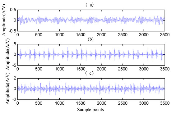
Figure 10.
The collected vibration signals: (a) normal signal; (b) outer race fault signal; and (c) inner race fault signal.
In order to illustrate the effect of this scheme on noise processing, the mean and standard deviation of ambiguity correlation coefficients based on EWT and EMD are calculated respectively. The results are shown in Table 3 and Table 4.
Table 3.
The mean and standard deviation based on EMD.
Table 4.
The mean and standard deviation based on EWT.
There were three sets of data 1#, 2#, and 3#, whose types were known as normal state signal, outer race fault signal, and inner race fault signal, respectively. The ambiguity correlation coefficients between normal working state signal and three known types of signals were calculated, and the mean and variance of the correlation coefficients were counted. Similarly, the ambiguity correlation coefficients between the outer race fault signal, the inner race fault signal, and the three known types of signals were calculated, respectively, and the mean and variance of the correlation coefficients were counted. The mean and standard deviation based on EMD are shown in Table 3, and the mean and standard deviation based on EWT are shown in Table 4. Comparing the data in Table 3 and Table 4, we find that in Table 4, the correlation coefficient between the rolling bearing signal and the same type of data set is always the largest, regardless of the working conditions of the rolling bearing. On the other hand, in Table 3, the identification of the bearing’s working condition is not obvious. Even when the rolling bearing is in the outer race fault state, the correlation coefficient between the rolling bearing signal and the 1# data set (the normal signal data set) is greater than that between the rolling bearing signal and the 2# data set (outer race fault data set). That is to say, the probability of identifying errors is very large at this time. The modal aliasing phenomenon exists in the decomposed signals by EMD, so the ambiguity correlation coefficients of the three decomposed signals are not distinguished clearly, and even produce errors. The information obtained by EWT decomposition is more effective, and the classification of signals can be clearly separated by ambiguity correlation coefficient. The normal distribution curves of the above results are shown in Figure 11 and Figure 12.
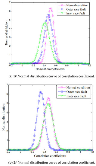
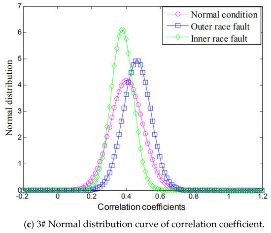
Figure 11.
Normal Distribution of EMD.
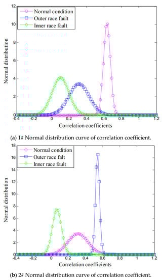
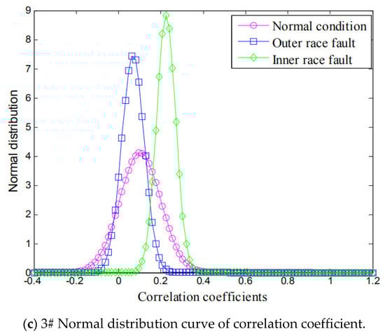
Figure 12.
Normal Distribution of EWT.
Figure 11 and Figure 12 show more clearly the two methods for the identification of the three working conditions of the rolling bearing: the center of normal distribution of correlation coefficient based on EWT can well identify the signals produced by rolling bearings in different working conditions, while the normal distribution curve discrimination based on EMD correlation coefficient is not obvious or even wrong in signal recognition.
Both back propagation (BP) neural network and support vector machine (SVM) are commonly used classifiers. We compared the proposed scheme with the two, taking 20 sets of data for training and testing, 15 of which were trained and five of which were used as test data. The test results are shown in Table 5.
Table 5.
The classification accuracy of three classifiers.
As can be seen from Table 5, the method proposed in this paper is superior to BP and SVM classifiers in classification accuracy. At the same time, the method proposed in this paper has short training time and no parameter adjustment problems, and can diagnose different working states of rolling bearings.
5. Conclusions
According to the non-linear and non-stationary characteristics of rolling bearing signals mixed with a large number of Gaussian noises, the method presented in this paper has the following characteristics:
- (1)
- Using EWT to decompose the vibration signal, the exact component can be obtained, and the mode aliasing phenomenon can be eliminated compared with EMD decomposition.
- (2)
- The sub-modes of EWT are tested by Gaussian distribution hypothesis to identify Gaussian noise. This method does not have parameter selection and has good adaptability.
- (3)
- Aiming at the shortcomings of traditional BP and SVM classifiers, such as too many parameters and slow convergence speed, the proposed classifier does not need parameter settings, and the calculation is simple. The experimental results show that the classifier can monitor different working conditions of rolling bearings, and the recognition rate is higher than BP and SVM.
Author Contributions
M.G., K.B. and X.R. conceived and designed the experiments; M.G. performed the experiments and analyzed the data; J.W., F.Z. and Y.X. provided guidance and recommendations for this research.
Funding
This research received no external funding.
Conflicts of Interest
The authors declare no conflict of interest.
References
- Laha, S.K. Enhancement of fault diagnosis of rolling element bearing using maximum kurtosis fast nonlocal means denoising. Measurement 2017, 100, 157–163. [Google Scholar] [CrossRef]
- Chen, X.W.; Feng, Z.P. Time-frequency analysis of torsional vibration signals in resonance region for planetary gearbox fault diagnosis under variable speed conditions. IEEE Access 2017, 5, 21918–21926. [Google Scholar] [CrossRef]
- Jiang, L.; Yin, H.; Li, X.; Tang, S. Fault diagnosis of rotating machinery based on multi sensor information fusion using svm and time-domain features. Shock Vib. 2014, 2014, 418178. [Google Scholar]
- Yuan, R.; Lv, Y.; Song, G. Multi-fault diagnosis of rolling bearings via adaptive projection intrinsically transformed multivariate empirical mode decomposition and high order singular value decomposition. Sensors 2018, 18, 1210. [Google Scholar] [CrossRef] [PubMed]
- Tiwari, R.; Gupta, V.K.; Kankar, P.K. Bearing fault diagnosis based on multi-scale permutation entropy and adaptive neuro fuzzy classifier. J. Vib. Control 2013, 21, 461–467. [Google Scholar] [CrossRef]
- Ge, M.; Wang, J.; Ren, X. Fault Diagnosis of Rolling Bearings Based on EWT and KDEC. Entropy 2017, 19, 633. [Google Scholar] [CrossRef]
- Zhao, H.; Pan, Z.; Ye, J. A rolling bearing compound fault diagnosis method based on nonlinear manifold. Mech. Transm. 2012, 7, 89–91. (In Chinese) [Google Scholar]
- Zhou, H.; Shi, T.; Liao, G.; Xuan, J.; Duan, J.; Su, L.; He, Z.; Lai, W. Weighted Kernel Entropy Component Analysis for Fault Diagnosis of Rolling Bearings. Sensors 2017, 17, 625. [Google Scholar] [CrossRef]
- He, Z.J.; Zi, Y.Y.; Meng, Q.F. Fault Diagnosis Principles of Non-Stationary Signal and Applications to Mechanical Equipment; Higher Education Press: Beijing, China, 2001; pp. 1–9. ISBN 704010284. [Google Scholar]
- Hao, R.; Lu, W.; Chu, F. Mathematical morphology extraction method for rolling bearing fault signals. Chin. J. Electr. Eng. 2008, 28, 65–70. (In Chinese) [Google Scholar]
- Li, C.; Zhang, X.; Zhou, D.; Guo, X.; Zhang, L. Fault diagnosis of rolling bearing based on bispectrum fuzzy clustering. J. Nantong Univ. (Nat. Sci. Ed.) 2014, 13, 32–36. [Google Scholar]
- Cai, J.H.; Hu, W.W.; Wang, X.H. Based on higher-order statistics, rolling bearing fault diagnosis method. J. Vib. Meas. Diagn. 2013, 33, 298–301. [Google Scholar]
- Azzalini, A.; Farge, M.; Kai, S. Nonlinear wavelet thresholding: A recursive method to determine the optimal denoising threshold. Appl. Comput. Harmon Aanl. 2005, 18, 177–185. [Google Scholar] [CrossRef]
- Kankar, P.K.; Sharma, S.C.; Harsha, S.P. Rolling element bearing fault diagnosis using wavelet transform. Neurocomputing 2011, 74, 1638–1645. [Google Scholar] [CrossRef]
- Kumar, A.; Kumar, R. Enhancing Weak Defect Features Using Undecimated and Adaptive Wavelet Transform for Estimation of Roller Defect Size in a Bearing. Tribol. Trans. 2017, 5, 60. [Google Scholar] [CrossRef]
- Luisier, F.; Blu, T. SURE-LET multichannel image denoising: Interscale orthonormal wavelet thresholding. IEEE Trans. Image Process. 2008, 17, 482–492. [Google Scholar] [CrossRef]
- Xu, Y.; Liang, F.; Zhang, G.; Xu, H. Image Intelligent Detection Based on the Gabor Wavelet and the Neural Network. Symmetry 2016, 8, 130. [Google Scholar] [CrossRef]
- Zhen, R.; Zhengping, Z.; Wenying, H. Denoising and detection of faulted motor signal based on best wavelet packet basis. Proc. CSEE 2002, 2, 53–57. [Google Scholar]
- Yang, P.; Yang, Q. Empirical Mode Decomposition and Rough Set Attribute Reduction for Ultrasonic Flaw Signal Classification. Int. J. Comput. Intell. Syst. 2014, 7, 481–492. [Google Scholar] [CrossRef]
- Deng, W.; Zhao, H.; Yang, X.; Dong, C. A Fault Feature Extraction Method for Motor Bearing and Transmission Analysis. Symmetry 2017, 9, 60. [Google Scholar] [CrossRef]
- Wang, W.; Chau, K.; Xu, D.; Chen, X.-Y. Improving forecasting accuracy of annual runoff time series using ARIMA based on EEMD decomposition. Water Resour. Manag. 2015, 29, 2655–2675. [Google Scholar] [CrossRef]
- Sun, J.; Xiao, Q.; Wen, J.; Wang, F. Natural gas pipeline small leakage feature extraction and recognition based on LMD envelope spectrum entropy and SVM. Measurement 2014, 55, 434–443. [Google Scholar] [CrossRef]
- Gilles, J. Empirical wavelet transforms. IEEE Trans. Signal Process 2013, 61, 3999–4010. [Google Scholar] [CrossRef]
- Stein, S. Algorithms for ambiguity function processing. IEEE Trans. Acoust. Speech Signal Process. 2003, 29, 588–599. [Google Scholar] [CrossRef]
- Zhang, L.; Yang, B.; Luo, M. Joint Delay and Doppler Shift Estimation for Multiple Targets Using Exponential Ambiguity Function. IEEE Trans. Signal Process. 2017, 65, 2151–2163. [Google Scholar] [CrossRef]
- Lyu, X.; Stove, A.; Gashinova, M.; Cherniakov, M. Ambiguity function of Inmarsat BGAN signal for radar application. Electron. Lett. 2016, 52, 1557–1559. [Google Scholar] [CrossRef]


© 2018 by the authors. Licensee MDPI, Basel, Switzerland. This article is an open access article distributed under the terms and conditions of the Creative Commons Attribution (CC BY) license (http://creativecommons.org/licenses/by/4.0/).