Some Exact Solutions and Conservation Laws of the Coupled Time-Fractional Boussinesq-Burgers System

Abstract

In this paper, we investigate the invariant properties of the coupled time-fractional Boussinesq-Burgers system. The coupled time-fractional Boussinesq-Burgers system is established to study the fluid flow in the power system and describe the propagation of shallow water waves. Firstly, the Lie symmetry analysis method is used to consider the Lie point symmetry, similarity transformation. Using the obtained symmetries, then the coupled time-fractional Boussinesq-Burgers system is reduced to nonlinear fractional ordinary differential equations (FODEs), with $Erd\acute{e}lyi$-$Kober$ fractional differential operator. Secondly, we solve the reduced system of FODEs by using a power series expansion method. Meanwhile, the convergence of the power series solution is analyzed. Thirdly, by using the new conservation theorem, the conservation laws of the coupled time-fractional Boussinesq-Burgers system is constructed. In particular, the presentation of the numerical simulations of q-homotopy analysis method of coupled time fractional Boussinesq-Burgers system is dedicated.

1. Introduction

Fractional differential equations (FDEs) come from the generalization of classical differential equations of integer order. It is well known that fractional calculus was widely applied to describe many complex nonlinear phenomena arising in the areas of heat transfer, diffusion, solid mechanics, wave propagation and other topics. Therefore, the fractional partial differential equations play an important role in describing physics, engineering and other scientific fields [1,2,3,4].

In 2009, Gazizov and Kasatkin [5] extended Lie symmetry approach to investigate several FDEs. Based on the symmetry, many useful properties of FDEs, such as symmetry generators, similarity transformation, explicit solutions and conservation laws which can be analyzed successively [6,7,8,9,10,11,12,13,14,15,16,17,18,19,20]. Komal and Gupta [21,22] extended the symmetry approach from single time fractional PDEs to nonlinear systems of time fractional PDEs. The famous Noether theorem [23] established a connection between Lie symmetries and conservation laws of differential equations. Recently, constructing conservation laws via a new conservation Noether theorem to the FPDEs without Lagrangian has been introduced [24,25]. In spite of the symmetry approach and conservation laws have made some progress in FDEs, the research for coupled time fractional FDEs are not very well explored. There are still many unknown results having not been reported before. The main aim of this paper is to investigate the Lie point symmetry, similarity reduction and conservation laws under the definition of Riemann-Liouville fractional differential. In addition, numerical results and verification of the correctness of the presented method are presented. In this paper, the fractional Lie symmetry scheme and the new conservation Noether theorem are developed to research the coupled time-fractional Boussinesq-Burgers system, that is [26]

$$\begin{array}{c}\hfill \left\{\begin{array}{c}{D}_t^{\alpha }u-\frac{1}{2}{v}_x+2u{u}_x=0,\hfill \\ D_t^{\alpha }v-\frac{1}{2}{u}_{xxx}+2{(uv)}_x=0,\hfill \end{array}\right.\end{array}$$

(1)

where $0<\alpha \le 1$, $t>0$. $\frac{{\partial }^{\alpha }f(x,t)}{\partial t^{\alpha }}$ is the Riemann-Liouville partial fractional derivative, $u(x,t)$ is the horizontal velocity field and $v(x,t)$ is the height of the water surface above a horizontal level at the bottom. The coupled time-fractional Boussinesq-Burgers system is an interesting mathematical model that arises in the study of fluids flow in a dynamic system and describes the propagation of shallow water waves.

The organization of the paper is as follows. In Section 2, we recall some definitions of fractional derivatives given in [27,28,29,30,31,32,33,34,35,36,37,38]; we highlight some steps for the Lie symmetry analysis of PDEs. In Section 3, we obtain the Lie point symmetries and symmetry reductions of Equation (1). In Section 4, explicit solutions of reduction equation for Equation (1) are obtained by using the power series expansion method. In addition, the convergence of power series solution is analyzed. Section 5 deals with the application of the proposed approach for investigating conservation laws for Equation (1). In Section 6, the well-known q-homotopy analysis method is used to investigate numerical approximations for the coupled time fractional Boussinesq-Burgers system. The concluding remarks are presented in the last section.

2. Preliminaries

In this section, we discuss the main points of fractional Lie symmetry analysis of the coupled time fractional PDEs. Consider a system of time fractional PDEs as follows:

$$\begin{array}{c}\frac{{\partial }^{\alpha }u}{\partial t^{\alpha }}=F_1(x,t,u,v,u_x,v_x,u_{xx},v_{xx,\cdots }),\hfill \\ \frac{{\partial }^{\alpha }v}{\partial t^{\alpha }}=F_2(x,t,u,v,u_x,v_x,u_{xx},v_{xx,\cdots }),\hfill \end{array}$$

(2)

where $\alpha >0$, subscripts represent partial derivatives.

Definition 1

([29,30,31,32,33,34,35,36,37,38]). The Riemann-Liouville partial fractional derivative $\frac{{\partial }^{\alpha }f(x,t)}{\partial t^{\alpha }}$ is defined as follows:

$$D_t^{\alpha }f(x,t)=\frac{{\partial }^{\alpha }f(x,t)}{\partial t^{\alpha }}=\left\{\begin{array}{cc}\frac{1}{\mathrm{\Gamma }(n-\alpha )}\frac{{\partial }^n}{\partial t^n}{\int }_0^t{(t-s)}^{n-\alpha -1}f(x,s)ds,\hfill & t>0,n-1<\alpha <n\in N,\hfill \\ \frac{{\partial }^{n}f(x,t)}{\partial t^n},\hfill & \alpha =n\in N,\hfill \end{array}\right.$$

(3)

where $\mathrm{\Gamma }(\alpha )$ is the Euler’s gamma function. According to the Riemann-Liouville partial fractional derivative operators, we have

$$\begin{array}{c}{(D_t^{\alpha })}^{*}={(-1)}^n{I}_c^{n-\alpha }(D_t^n)={(D_c^{\alpha })}_t^C,\hfill \\ I_c^{n-\alpha }f(x,t)=\frac{1}{\mathrm{\Gamma }(n-\alpha )}{\int }_t^c\frac{f(x,s)}{{(s-t)}^{1+\alpha -n}}ds.forn=[\alpha ]+1,\hfill \end{array}$$

(4)

where ${(D_t^{\alpha })}^{*}$ is the adjoint operator for the $D_t^{\alpha }$, and ${(D_c^{\alpha })}_t^C$ is the right-sided Caputo operator [39,40]. Then we consider the single parameter Lie group with infinitesimal transformation given by

$$\begin{array}{c}\tilde{x}=x+\epsilon \xi (x,t,u,v)+o({\epsilon }^2),\hfill \\ \tilde{t}=t+\epsilon \tau (x,t,u,v)+o({\epsilon }^2),\hfill \\ \tilde{u}=u+\epsilon \eta (x,t,u,v)+o({\epsilon }^2),\hfill \\ \tilde{v}=v+\epsilon \varphi (x,t,u,v)+o({\epsilon }^2),\hfill \\ \frac{{\partial }^{\alpha }\tilde{u}}{\partial {\tilde{t}}^{\alpha }}=\frac{{\partial }^{\alpha }u}{\partial t^{\alpha }}+\epsilon {\eta }^{\alpha ,t}(x,t,u,v)+o({\epsilon }^2),\hfill \\ \frac{{\partial }^{\alpha }\tilde{v}}{\partial {\tilde{t}}^{\alpha }}=\frac{{\partial }^{\alpha }v}{\partial t^{\alpha }}+\epsilon {\varphi }^{\alpha ,t}(x,t,u,v)+o({\epsilon }^2),\hfill \\ \frac{\partial \tilde{u}}{\partial \tilde{x}}=\frac{\partial u}{\partial x}+\epsilon {\eta }^x(x,t,u,v)+o({\epsilon }^2),\hfill \\ \frac{\partial \tilde{v}}{\partial \tilde{x}}=\frac{\partial v}{\partial x}+\epsilon {\varphi }^x(x,t,u,v)+o({\epsilon }^2),\hfill \\ \frac{{\partial }^2\tilde{u}}{\partial {\tilde{x}}^2}=\frac{{\partial }^{2}u}{\partial x^2}+\epsilon {\eta }^{xx}(x,t,u,v)+o({\epsilon }^2),\hfill \\ \frac{{\partial }^2\tilde{v}}{\partial {\tilde{x}}^2}=\frac{{\partial }^{2}v}{\partial x^2}+\epsilon {\varphi }^{xx}(x,t,u,v)+o({\epsilon }^2),\hfill \\ \frac{{\partial }^3\tilde{u}}{\partial {\tilde{x}}^3}=\frac{{\partial }^{3}u}{\partial x^3}+\epsilon {\eta }^{xxx}(x,t,u,v)+o({\epsilon }^2),\hfill \\ \frac{{\partial }^3\tilde{v}}{\partial {\tilde{x}}^3}=\frac{{\partial }^{3}v}{\partial x^3}+\epsilon {\varphi }^{xxx}(x,t,u,v)+o({\epsilon }^2),\hfill \\ \hfill \end{array}$$

(5)

here ξ, τ, η and ϕ are the infinitesimals operators, ${\eta }^{\alpha ,t}$, ${\varphi }^{\alpha ,t}$ are the extended infinitesimal of order α and ${\eta }^x$, ${\varphi }^x$, ${\eta }^{xx}$, ${\varphi }^{xx}$,${\eta }^{xxx}$, ${\varphi }^{xxx}$ are extended infinitesimals of integer-order. Consider the following vector fields:

$$X=\xi (x,t,u,v)\frac{\partial }{\partial x}+\tau (x,t,u,v)\frac{\partial }{\partial t}+\eta (x,t,u,v)\frac{\partial }{\partial u}+\varphi (x,t,u,v)\frac{\partial }{\partial v}.$$

(6)

The αth order developed infinitesimal ${\eta }^{\alpha ,t}$ has the following form

$${\eta }^{\alpha ,t}=D_t^{\alpha }(\eta )+\xi D_t^{\alpha }(u_x)-D_t^{\alpha }(\xi u_x)+D_t^{\alpha }(D_t(\tau )u)-D_t^{\alpha +1}(\tau u)+\tau D_t^{\alpha +1}(u).$$

(7)

Using the generalized Leibnitz rule and generalized chain rule [41,42,43,44], the final expression for αth order developed infinitesimal ${\eta }^{\alpha ,t}$ for system of fractional PDEs of the form Equation (2) can be calculated as follows:

$$\begin{array}{cc}\hfill {\eta }^{\alpha ,t}=& \frac{{\partial }^{\alpha }\eta }{\partial t^{\alpha }}+({\eta }_u-\partial D_t(\tau ))\frac{{\partial }^{\alpha }u}{\partial t^{\alpha }}-u\frac{{\partial }^{\alpha }{\eta }_u}{\partial t^{\alpha }}+({\eta }_v\frac{{\partial }^{\alpha }v}{\partial t^{\alpha }}-v\frac{{\partial }^{\alpha }{\eta }_v}{\partial t^{\alpha }})+{\mu }_1+{\mu }_2+\sum _{n=1}^{\infty }[\left(\genfrac{}{}{0pt}{}{\alpha }{n}\right)\frac{{\partial }^n{\eta }_u}{\partial t^n}-\hfill \\ & \left(\genfrac{}{}{0pt}{}{\alpha }{n+1}\right)D_t^{n+1}(\tau )]D_t^{\alpha -n}(u)+\sum _{n=1}^{\infty }\left(\genfrac{}{}{0pt}{}{\alpha }{n}\right)\frac{{\partial }^n{\eta }_v}{\partial t^n}{D}_t^{\alpha -n}(v)-\sum _{n=1}^{\infty }\left(\genfrac{}{}{0pt}{}{\alpha }{n}\right)D_t^n(\xi )D_t^{\alpha -n}(u_x),\hfill \\ \hfill {\varphi }^{\alpha ,t}=& \frac{{\partial }^{\alpha }\varphi }{\partial t^{\alpha }}+({\varphi }_v-\partial D_t(\tau ))\frac{{\partial }^{\alpha }v}{\partial t^{\alpha }}-v\frac{{\partial }^{\alpha }{\varphi }_v}{\partial t^{\alpha }}+({\varphi }_u\frac{{\partial }^{\alpha }u}{\partial t^{\alpha }}-u\frac{{\partial }^{\alpha }{\varphi }_u}{\partial t^{\alpha }})+{\mu }_3+{\mu }_4+\sum _{n=1}^{\infty }[\left(\genfrac{}{}{0pt}{}{\alpha }{n}\right)\frac{{\partial }^n{\varphi }_v}{\partial t^n}-\hfill \\ & \left(\genfrac{}{}{0pt}{}{\alpha }{n+1}\right)D_t^{n+1}(\tau )]D_t^{\alpha -n}(v)+\sum _{n=1}^{\infty }\left(\genfrac{}{}{0pt}{}{\alpha }{n}\right)\frac{{\partial }^n{\varphi }_u}{\partial t^n}{D}_t^{\alpha -n}(u)-\sum _{n=1}^{\infty }\left(\genfrac{}{}{0pt}{}{\alpha }{n}\right)D_t^n(\xi )D_t^{\alpha -n}(v_x),\hfill \end{array}$$

(8)

where $D_t$ represents the total derivative operator, ${\mu }_1$, ${\mu }_2$, ${\mu }_3$, ${\mu }_4$ are given by

$$\begin{array}{c}{\mu }_1=\sum _{n=2}^{\infty }\sum _{m=2}^n\sum _{k=2}^m\sum _{r=0}^{k-1}\left(\genfrac{}{}{0pt}{}{\alpha }{n}\right)\left(\genfrac{}{}{0pt}{}{n}{m}\right)\left(\genfrac{}{}{0pt}{}{k}{r}\right)\frac{1}{k!}\frac{t^{n-\alpha }}{\mathrm{\Gamma }(n-\alpha +1)}{(-u)}^r\frac{{\partial }^m}{\partial t^m}(u^{k-r})\frac{{\partial }^{n-m+k}\eta }{\partial t^{n-m}\partial u^k},\hfill \\ {\mu }_2=\sum _{n=2}^{\infty }\sum _{m=2}^n\sum _{k=2}^m\sum _{r=0}^{k-1}\left(\genfrac{}{}{0pt}{}{\alpha }{n}\right)\left(\genfrac{}{}{0pt}{}{n}{m}\right)\left(\genfrac{}{}{0pt}{}{k}{r}\right)\frac{1}{k!}\frac{t^{n-\alpha }}{\mathrm{\Gamma }(n-\alpha +1)}{(-v)}^r\frac{{\partial }^m}{\partial t^m}(v^{k-r})\frac{{\partial }^{n-m+k}\eta }{\partial t^{n-m}\partial v^k},\hfill \\ {\mu }_3=\sum _{n=2}^{\infty }\sum _{m=2}^n\sum _{k=2}^m\sum _{r=0}^{k-1}\left(\genfrac{}{}{0pt}{}{\alpha }{n}\right)\left(\genfrac{}{}{0pt}{}{n}{m}\right)\left(\genfrac{}{}{0pt}{}{k}{r}\right)\frac{1}{k!}\frac{t^{n-\alpha }}{\mathrm{\Gamma }(n-\alpha +1)}{(-u)}^r\frac{{\partial }^m}{\partial t^m}(u^{k-r})\frac{{\partial }^{n-m+k}\varphi }{\partial t^{n-m}\partial u^k},\hfill \\ {\mu }_4=\sum _{n=2}^{\infty }\sum _{m=2}^n\sum _{k=2}^m\sum _{r=0}^{k-1}\left(\genfrac{}{}{0pt}{}{\alpha }{n}\right)\left(\genfrac{}{}{0pt}{}{n}{m}\right)\left(\genfrac{}{}{0pt}{}{k}{r}\right)\frac{1}{k!}\frac{t^{n-\alpha }}{\mathrm{\Gamma }(n-\alpha +1)}{(-v)}^r\frac{{\partial }^m}{\partial t^m}(v^{k-r})\frac{{\partial }^{n-m+k}\varphi }{\partial t^{n-m}\partial v^k}.\hfill \\ \hfill \end{array}$$

(9)

Equation (5) represents a point symmetry of Equation (2) as long as

$$P_r^{\alpha ,i}X(▵){\mid }_{▵=0}=0,$$

(10)

where i is the order of system Equation (5). The invariance condition should be held:

$$\tau (x,t,u,v){\mid }_{t=0}=0.$$

(11)

3. Symmetry Analysis

3.1. Lie Symmetry Analysis

Let us consider the invariance of the group transformations (5). The invariance criterion takes the following forms:

$$\begin{array}{c}{\eta }_1^{\alpha ,t}-\frac{1}{2}{\varphi }^x+2(u{\eta }^x+\eta u_x)=0,\hfill \\ {\eta }_2^{\alpha ,t}-\frac{1}{2}{\eta }^{xxx}+2({\eta }^{x}v+u_x\varphi +\eta v_x+u{\varphi }^x)=0.\hfill \end{array}$$

(12)

Then, substituting the values of prolongations and equating the coefficients of various linearly independent variables to zero, we have:

$$\xi =\frac{c_{1}x}{2}+c_2,\tau =\frac{c_{1}t}{\alpha },\eta =-\frac{c_1}{2}u,\varphi =-c_{1}v,$$

(13)

where $c_1$, $c_2$ are arbitrary constants.

Therefore, one infers the following corresponding infinitesimal generators of Lie algebra:

$$V_1=\frac{x}{2}\frac{\partial }{\partial x}+\frac{t}{\partial }\frac{\partial }{\partial t}-\frac{1}{2}u\frac{\partial }{\partial u}-v\frac{\partial }{\partial v},V_2=\frac{\partial }{\partial x}.$$

(14)

It is easy to check that the vector fields (14) are closed under the Lie bracket, respectively

$$[V_1,V_1]=0=[V_2,V_2],[V_1,V_2]=-\frac{1}{2}{V}_2=-[V_2,V_1].$$

(15)

Considering the vector field $V_1$, we can write the characteristic equations

$$\begin{array}{c}\hfill \frac{dx}{\frac{x}{2}}=\frac{dt}{\frac{t}{\alpha }}=\frac{du}{-\frac{u}{2}}=\frac{dv}{-v}.\end{array}$$

(16)

Solving the above equations, the similarity solutions are given by

$$\begin{array}{c}\hfill \omega =x{t}^{-\frac{\alpha }{2}},u(x,t)=t^{-\frac{\alpha }{2}}f(\omega ),v(x,t)=t^{-\alpha }g(\omega ).\end{array}$$

(17)

3.2. Symmetry Reductions

In order to obtain the symmetry reductions of Equation (1), we apply the $Erd\acute{e}lyi$-$Kober$ fractional differential operator $({\phi }_{\delta }^{\xi ,\alpha })$.

Definition 2

([45,46,47]).

$$({\phi }_{\delta }^{\xi ,\alpha }h)(\omega )={\Pi }_{j=0}^{m-1}(\xi +j-\frac{1}{\delta }w\frac{d}{d\omega })({\kappa }_{\delta }^{\xi +\alpha ,m-\alpha }h)(\omega ),m=\left\{\begin{array}{cc}[\alpha ]+1,\hfill & if\alpha \notin N,\hfill \\ \alpha ,\hfill & if\alpha \in N,\hfill \end{array}\right.$$

(18)

where

$$\begin{array}{c}\hfill ({\kappa }_{\delta }^{\xi ,\alpha }h)(\omega ):=\left\{\begin{array}{cc}\frac{1}{\mathrm{\Gamma }(\alpha )}{\int }_1^{\infty }{(p-1)}^{\alpha -1}{p}^{-(\xi +\alpha )}h(\omega p^{\frac{1}{\delta }})dp,\hfill & if\alpha >0,\hfill \\ h(\omega ),\hfill & if\alpha =0,\hfill \end{array}\right.\end{array}$$

(19)

is the $Erd\acute{e}lyi$-$Kober$ fractional integral operator. To calculated $\frac{{\partial }^{\alpha }u}{\partial t^{\alpha }}$, first let $n-1<\alpha <n(n=1,2,3,\cdots )$, with the help of similarity transformation $u(x,t)=t^{-\frac{\alpha }{2}}f(\omega )$, $v(x,t)=t^{-\alpha }g(\omega )$ and similarity variable $\omega =x{t}^{-\frac{\alpha }{2}}$, the definition of Riemann-Liouville fractional derivative (3) can be written as following:

$$\frac{{\partial }^{\alpha }u}{\partial t^{\alpha }}=\frac{{\partial }^n}{\partial t^n}[\frac{1}{\mathrm{\Gamma }(n-\alpha )}{\int }_0^t{(t-s)}^{n-\alpha -1}{s}^{-\frac{\alpha }{2}}f(x{s}^{-\frac{\alpha }{2}})ds].$$

(20)

Let $p=\frac{t}{s}$, then the above expression is converted to the following:

$$\frac{{\partial }^{\alpha }u}{\partial t^{\alpha }}=\frac{{\partial }^n}{\partial t^n}[\frac{t^{n-\frac{3}{2}\alpha }}{\mathrm{\Gamma }(n-\alpha )}{\int }_1^{\infty }{(p-1)}^{n-\alpha -1}{p}^{-(n-\frac{3}{2}\alpha +1)}f(\omega p^{\frac{\alpha }{2}})dp].$$

(21)

Based on the definition of $Erd\acute{e}lyi$-$Kober$ fractional integral operator, (21) can be written as

$$\frac{{\partial }^{\alpha }u}{\partial t^{\alpha }}=\frac{{\partial }^n}{\partial t^n}[t^{n-\frac{3}{2}\alpha }({\kappa }_{\frac{2}{\alpha }}^{1-\frac{\alpha }{2},n-\alpha }f)(\omega )].$$

(22)

Considering $\psi (\omega )=C^1(0,\infty )$ for $\omega =x{t}^{-\frac{\alpha }{2}}$, it holds that

$$t\frac{\partial }{\partial t}\psi (\omega )=-\frac{\alpha }{2}\omega \frac{d}{d\omega }\psi (\omega ).$$

(23)

Hence, Equation (22) can be transformed as follows:

$$\begin{array}{c}\frac{{\partial }^n}{\partial t^n}[t^{n-\frac{3}{2}\alpha }({\kappa }_{\frac{2}{\alpha }}^{1-\frac{\alpha }{2},n-\alpha }f)(\omega )]\hfill \\ =\frac{{\partial }^{n-1}}{\partial t^{n-1}}[\frac{\partial }{\partial t}(t^{n-\frac{3}{2}\alpha }({\kappa }_{\frac{2}{\alpha }}^{1-\frac{\alpha }{2},n-\alpha }f)(\omega ))]\hfill \\ =\frac{{\partial }^{n-1}}{\partial t^{n-1}}[(n-\frac{3}{2}\alpha )t^{n-\frac{3}{2}\alpha -1}({\kappa }_{\frac{2}{\alpha }}^{1-\frac{\alpha }{2},n-\alpha }f)(\omega )+t^{n-\frac{3}{2}\alpha -1}(-\frac{\alpha }{2}\omega \frac{d}{d\omega })({\kappa }_{\frac{2}{\alpha }}^{1-\frac{\alpha }{2},n-\alpha }f)(\omega )]\hfill \\ =\frac{{\partial }^{n-1}}{\partial t^{n-1}}[t^{n-\frac{3}{2}\alpha -1}(n-\frac{3}{2}\alpha -\frac{\alpha }{2}\omega \frac{d}{d\omega })({\kappa }_{\frac{2}{\alpha }}^{1-\frac{\alpha }{2},n-\alpha }f)(\omega )]\hfill \\ =t^{-\frac{3}{2}\alpha }{\Pi }_{j=0}^{n-1}(1-\frac{3}{2}\alpha +j-\frac{\alpha }{2}\omega \frac{d}{d\omega })({\kappa }_{\frac{2}{\alpha }}^{1-\frac{\alpha }{2},n-\alpha }f)(\omega )\hfill \\ =t^{-\frac{3}{2}\alpha }({\phi }_{\frac{2}{\alpha }}^{1-\frac{3}{2}\alpha ,\alpha }f)(\omega ).\hfill \end{array}$$

(24)

According to the definition of $Erd\acute{e}lyi$-$Kober$ fractional differential operator, it can be written as follows:

$$\frac{{\partial }^{\alpha }u}{\partial t^{\alpha }}=t^{-\frac{3}{2}\alpha }({\phi }_{\frac{2}{\alpha }}^{1-\frac{3}{2}\alpha ,\alpha }f)(\omega ).$$

(25)

At the same time, the $\frac{{\partial }^{\alpha }v}{\partial t^{\alpha }}$ can be presented as

$$\frac{{\partial }^{\alpha }v}{\partial t^{\alpha }}=t^{-2\alpha }({\phi }_{\frac{2}{\alpha }}^{1-2\alpha ,\alpha }g)(\omega ).$$

(26)

In the case $\alpha =1,2,3,\cdots$, $\omega =x{t}^{-\frac{n}{2}}$, we have the following:

$$\begin{array}{cc}\hfill \frac{{\partial }^{\alpha }u}{\partial t^{\alpha }}& =\frac{{\partial }^n}{\partial t^n}(t^{-\frac{n}{2}}f(\omega ))=\frac{{\partial }^{n-1}}{\partial t^{n-1}}[\frac{\partial }{\partial t}(t^{-\frac{n}{2}}f(\omega ))]\hfill \\ & =\frac{{\partial }^{n-1}}{\partial t^{n-1}}[t^{-\frac{n}{2}-1}(-\frac{n}{2}-\frac{\alpha }{2}\omega \frac{d}{d\omega })f(\omega )]\hfill \\ & =\cdots =t^{-\frac{3}{2}n}{\Pi }_{j=0}^{n-1}(1-\frac{3}{2}n+j-\frac{\alpha }{2}\omega \frac{d}{d\omega })f(\omega )\hfill \\ & =t^{-\frac{3}{2}n}({\phi }_{\frac{2}{n}}^{1-\frac{3}{2}n,n}f)(\omega ).\hfill \end{array}$$

(27)

Similarly, for $\alpha =n=1,2,3,\cdots$, we have $\frac{{\partial }^{\alpha }v}{\partial t^{\alpha }}=t^{-2n}({\phi }_{\frac{2}{n}}^{1-2n,n}g)(\omega )$. Hence, expressions (25) and (26) hold for $n-1<\alpha \le n$.

Therefore, the coupled time-fractional Boussinesq-Burgers system (1) is reduced to

$$\begin{array}{c}({\phi }_{\frac{2}{\alpha }}^{1-\frac{3}{2}\alpha ,\alpha }f)(\omega )-\frac{1}{2}{g}^{\prime }(\omega )+2f(\omega )f^{\prime }(\omega )=0,\hfill \\ ({\phi }_{\frac{2}{\alpha }}^{1-2\alpha ,\alpha }g)(\omega )-\frac{1}{2}{f}^{\prime \prime \prime }(\omega )+2f(\omega )g^{\prime }(\omega )+2f^{\prime }(\omega )g(\omega )=0.\hfill \end{array}$$

(28)

4. Power Series Solution

In what follows, we shall derive explicit solutions for system (1) by means of the power series expansion method. To find the exact power series solutions of system (1), we let

$$\begin{array}{c}f(\omega )=\sum _{n=0}^{\infty }{a}_n{\omega }^n,\hfill \\ g(\omega )=\sum _{n=0}^{\infty }{b}_n{\omega }^n,\hfill \end{array}$$

(29)

where $a_n$ and $b_n$ are constants to be known later. Substituting Equation (29) into Equation (28), we can obtain

$$\begin{array}{c}\sum _{n=0}^{\infty }\frac{\mathrm{\Gamma }(2-\frac{\alpha }{2}+\frac{n\alpha }{2})}{\mathrm{\Gamma }(2-\frac{3\alpha }{2}+\frac{n\alpha }{2})}{a}_n{\omega }^n-\frac{1}{2}\sum _{n=0}^{\infty }(n+1)b_{n+1}{\omega }^n+2\sum _{n=0}^{\infty }{a}_n{\omega }^n\sum _{n=0}^{\infty }(n+1)a_{n+1}{\omega }^n=0,\hfill \\ \sum _{n=0}^{\infty }\frac{\mathrm{\Gamma }(2-\alpha +\frac{n\alpha }{2})}{\mathrm{\Gamma }(2-2\alpha +\frac{n\alpha }{2})}{b}_n{\omega }^n-\frac{1}{2}\sum _{n=0}^{\infty }(n+2)(n+3)(n+1)a_{n+3}{\omega }^n+2\sum _{n=0}^{\infty }{a}_n{\omega }^n\sum _{n=0}^{\infty }(n+1)b_{n+1}{\omega }^n\hfill \\ +2\sum _{n=0}^{\infty }{b}_n{\omega }^n\sum _{n=0}^{\infty }(n+1)a_{n+1}{\omega }^n=0.\hfill \end{array}$$

(30)

In view of Equation (30), comparing coefficients for $n=0$, we get

$$\begin{array}{cc}\hfill b_1=& 2[\frac{\mathrm{\Gamma }(2-\frac{\alpha }{2})}{\mathrm{\Gamma }(2-\frac{3\alpha }{2})}+2a_0{a}_1],\hfill \\ \hfill a_3=& \frac{1}{3}[\frac{\mathrm{\Gamma }(2-\alpha )}{\mathrm{\Gamma }(2-2\alpha )}{b}_0+2a_0{b}_1+2b_0{a}_1].\hfill \end{array}$$

(31)

When $n\ge 1$, we have

$$\begin{array}{cc}\hfill b_{n+1}=& \frac{2}{n+1}[\frac{\mathrm{\Gamma }(2-\frac{\alpha }{2}+\frac{n\alpha }{2})}{\mathrm{\Gamma }(2-\frac{3\alpha }{2}+\frac{n\alpha }{2})}{a}_n+2\sum _{k=0}^n(n+1-k)a_k{a}_{n+1-k}],\hfill \\ \hfill a_{n+3}=& \frac{2}{(n+3)(n+2)(n+1)}[\frac{\mathrm{\Gamma }(2-\alpha +\frac{n\alpha }{2})}{\mathrm{\Gamma }(2-2\alpha +\frac{n\alpha }{2})}{b}_n+2\sum _{k=0}^n{a}_k(n+1-k)b_{n+1-k}\hfill \\ & +2\sum _{k=0}^n{b}_k(n+1-k)a_{n+1-k}].\hfill \end{array}$$

(32)

Then, we can write

$$\begin{array}{cc}\hfill f(\omega )=& a_0+a_1\omega +a_2{\omega }^2+\frac{1}{3}[\frac{\mathrm{\Gamma }(2-\alpha )}{\mathrm{\Gamma }(2-2\alpha )}{b}_0+2a_0{b}_1+2b_0{a}_1]{\omega }^3\hfill \\ & +\sum _{n=1}^{\infty }\frac{2}{(n+3)(n+2)(n+1)}[\frac{\mathrm{\Gamma }(2-\alpha +\frac{n\alpha }{2})}{\mathrm{\Gamma }(2-2\alpha +\frac{n\alpha }{2})}{b}_n\hfill \\ & +2\sum _{k=0}^n{a}_k(n+1-k)b_{n+1-k}+2\sum _{k=0}^n{b}_k(n+1-k)a_{n+1-k}]{\omega }^{n+3},\hfill \\ \hfill g(\omega )=& b_0+2[\frac{\mathrm{\Gamma }(2-\frac{\alpha }{2})}{\mathrm{\Gamma }(2-\frac{3\alpha }{2})}+2a_0{a}_1]\omega +\sum _{n=1}^{\infty }\frac{2}{n+1}[\frac{\mathrm{\Gamma }(2-\frac{\alpha }{2}+\frac{n\alpha }{2})}{\mathrm{\Gamma }(2-\frac{3\alpha }{2}+\frac{n\alpha }{2})}{a}_n\hfill \\ & +2\sum _{k=0}^n(n+1-k)a_k{a}_{n+1-k}]{\omega }^{n+1}.\hfill \end{array}$$

(33)

Hence, the explicit solution of Equation (1) is

$$\begin{array}{cc}\hfill u(x,t)=& a_0{t}^{-\frac{\alpha }{2}}+a_{1}x{t}^{-\alpha }+a_2{x}^2{t}^{-\frac{3\alpha }{2}}+\frac{1}{3}[\frac{\mathrm{\Gamma }(2-\alpha )}{\mathrm{\Gamma }(2-2\alpha )}{b}_0+2a_0{b}_1+2b_0{a}_1]x^3{t}^{-2\alpha }\hfill \\ & +\sum _{n=1}^{\infty }\frac{2}{(n+3)(n+2)(n+1)}[\frac{\mathrm{\Gamma }(2-\alpha +\frac{n\alpha }{2})}{\mathrm{\Gamma }(2-2\alpha +\frac{n\alpha }{2})}{b}_n+2\sum _{k=0}^n(n+1-k)a_k{b}_{n+1-k}\hfill \\ & +2\sum _{k=0}^n(n+1-k)b_k{a}_{n+1-k}]x^{n+3}{t}^{-\frac{(n+4)\alpha }{2}},\hfill \\ \hfill v(x,t)=& b_0{t}^{-\alpha }+2[\frac{\mathrm{\Gamma }(2-\frac{\alpha }{2})}{\mathrm{\Gamma }(2-\frac{3\alpha }{2})}+2a_0{a}_1]x{t}^{-\frac{3\alpha }{2}}+\sum _{n=1}^{\infty }\frac{2}{n+1}[\frac{\mathrm{\Gamma }(2-\frac{\alpha }{2}+\frac{n\alpha }{2})}{\mathrm{\Gamma }(2-\frac{3\alpha }{2}+\frac{n\alpha }{2})}{a}_n\hfill \\ & +2\sum _{k=0}^n(n+1-k)a_k{a}_{n+1-k}]x^{n+1}{t}^{-\frac{(n+3)\alpha }{2}}.\hfill \end{array}$$

(34)

(see Figure 1).

Convergence Analysis

In this part, the convergence of the power series solution of Equation (29) for Equation (28) will be investigated. Consider Equation (32) such that

$$\begin{array}{c}\mid b_{n+1}\mid \le [\frac{\mid \mathrm{\Gamma }(2-\frac{\alpha }{2}+\frac{n\alpha }{2})\mid }{\mid \mathrm{\Gamma }(2-\frac{3\alpha }{2}+\frac{n\alpha }{2})\mid }\mid a_n\mid +4\sum _{k=0}^n\mid a_k\mid \mid a_{n+1-k}\mid ],\hfill \\ \mid a_{n+3}\mid \le [\frac{\mid \mathrm{\Gamma }(2-\alpha +\frac{n\alpha }{2})\mid }{\mid \mathrm{\Gamma }(2-2\alpha +\frac{n\alpha }{2})\mid }\mid b_n\mid +\sum _{k=0}^n\mid a_k\mid \mid b_{n+1-k}\mid +\sum _{k=0}^n\mid b_k\mid \mid a_{n+1-k}\mid ].\hfill \end{array}$$

(35)

It is known that $\frac{\mid \mathrm{\Gamma }(n)\mid }{\mid \mathrm{\Gamma }(m)\mid }<1$, for arbitrary n and m. Thus Equation (35) becomes

$$\begin{array}{c}\mid b_{n+1}\mid \le M[\mid a_n\mid +\sum _{k=0}^n\mid a_k\mid \mid a_{n+1-k}\mid ],\hfill \\ \mid a_{n+3}\mid \le N[\mid b_n\mid +\sum _{k=0}^n\mid a_k\mid \mid b_{n+1-k}\mid +\sum _{k=0}^n\mid b_k\mid \mid a_{n+1-k}\mid ],\hfill \end{array}$$

(36)

where $M=max\{e_1,4e_2\}$, $N=max\{e_3,e_4,e_5\}$, $e_i(i=1,2,\cdots ,5)$ are arbitrary constants. Then, we introduce another power series

$$\begin{array}{c}R(\omega )=\sum _{n=0}^{\infty }{r}_n{\omega }^n,\hfill \\ Q(\omega )=\sum _{n=0}^{\infty }{q}_n{\omega }^n,\hfill \end{array}$$

(37)

by $r_i=\mid a_i\mid$, $q_i=\mid b_i\mid$, $i=0,1,2,\cdots$. Then we can have

$$\begin{array}{c}{r}_{n+1}\le M(r_n+\sum _{k=0}^n{r}_k{r}_{n+1-k}),\hfill \\ q_{n+3}\le N(q_n+\sum _{k=0}^n{r}_k{q}_{n+1-k}+\sum _{k=0}^n{q}_k{r}_{n+1-k}).\hfill \end{array}$$

(38)

Thus it is easily seen that $\mid r_n\mid \le a_n$, $\mid q_n\mid \le b_n$, $n=0,1,2,\cdots .$ In addition, the series $R(\omega )={\sum }_{n=0}^{\infty }{r}_n{\omega }^n$ and $Q(\omega )={\sum }_{n=0}^{\infty }{q}_n{\omega }^n$ are majorant series of Equation (40). By some calculation, we have

$$\begin{array}{c}R(\omega )=r_0+r_1\omega +r_2{\omega }^2+r_3{\omega }^3+N\sum _{n=0}^{\infty }{q}_n{\omega }^{n+3}+N\sum _{n=0}^{\infty }\sum _{k=0}^n{r}_k{q}_{n+1-k}{\omega }^{n+3}\hfill \\ +N\sum _{n=0}^{\infty }\sum _{k=0}^n{q}_k{r}_{n+1-k}{\omega }^{n+3},\hfill \\ Q(\omega )=q_0+q_1\omega +M\sum _{n=0}^{\infty }{r}_n{\omega }^{n+1}+M\sum _{n=0}^{\infty }\sum _{k=0}^n{r}_k{r}_{n+1-k}{\omega }^{n+1}.\hfill \end{array}$$

(39)

Then we consider the implicit function system with respect to the independent variable $\omega$

$$\begin{array}{c}R(\omega ,R)=R(\omega )-r_0-r_1\omega -r_2{\omega }^2-r_3{\omega }^3-N\sum _{n=0}^{\infty }{q}_n{\omega }^{n+3}-N\sum _{n=0}^{\infty }\sum _{k=0}^n{r}_k{q}_{n+1-k}{\omega }^{n+3}\hfill \\ -N\sum _{n=0}^{\infty }\sum _{k=0}^n{q}_k{r}_{n+1-k}{\omega }^{n+3}=0,\hfill \\ Q(\omega ,Q)=Q(\omega )-q_0-q_1\omega -M\sum _{n=0}^{\infty }{r}_n{\omega }^{n+1}-M\sum _{n=0}^{\infty }\sum _{k=0}^n{r}_k{r}_{n+1-k}{\omega }^{n+1}=0,\hfill \end{array}$$

(40)

since R and Q are analytic in a neighborhood of $(0,r)$ and $(0,q)$, where $R(0,r)=0$, $Q(0,q)=0$ and $\frac{\partial }{\partial R}(R(0,r))\ne 0$, $\frac{\partial }{\partial Q}(Q(0,q))\ne 0$. Then by the implicit function theorem [48], we reach the convergence.

5. Conservation Laws

The method of constructing conservation laws for fractional partial equations has been given in many papers [12,15,16,19,20,21,22,23,24]. In this section, we will study the conservation laws of the coupled time-fractional Boussinesq-Burgers system (1) by using the adjoint equation and symmetries of Equation (1). A formal Lagrangian for Equation (1) can be written in the following form:

$$\mathcal{L}=p(x,t)(\frac{{\partial }^{\alpha }u}{\partial t^{\alpha }}-\frac{1}{2}{v}_x+2u{u}_x)+q(x,t)(\frac{{\partial }^{\alpha }v}{\partial t^{\alpha }}+2{(uv)}_x),$$

(41)

where $p(x,t)$ and $q(x,t)$ are the new dependent variables. For Equation (1), the adjoint equation has the form

$$\begin{array}{c}\frac{\delta \mathcal{L}}{\delta u}=F_1^{*}={(D_t^{\alpha })}^{*}p-2u{p}_x-2q_{x}v+\frac{1}{2}{q}_{xxx},\hfill \\ \frac{\delta \mathcal{L}}{\delta v}=F_2^{*}={(D_t^{\alpha })}^{*}q+\frac{1}{2}{p}_x-2u{q}_x.\hfill \end{array}$$

(42)

Contenting ${\Xi }_i\ne 0$ with at least one $i(i=1,2)$, that is

$$\begin{array}{c}\frac{\delta \mathcal{L}}{\delta u}={\lambda }_1(\frac{{\partial }^{\alpha }u}{\partial t^{\alpha }}-\frac{1}{2}{v}_x+2u{u}_x)+{\lambda }_2(\frac{{\partial }^{\alpha }v}{\partial t^{\alpha }}+2{(uv)}_x-\frac{1}{2}{u}_{xxx}),\hfill \\ \frac{\delta \mathcal{L}}{\delta v}={\lambda }_3(\frac{{\partial }^{\alpha }u}{\partial t^{\alpha }}-\frac{1}{2}{v}_x+2u{u}_x)+{\lambda }_4(\frac{{\partial }^{\alpha }v}{\partial t^{\alpha }}+2{(uv)}_x-\frac{1}{2}{u}_{xxx}),\hfill \end{array}$$

(43)

where ${\lambda }_i(i=1,\cdots ,4)$ are undetermined coefficients. Using

$$p={\Xi }_1(x,t,u,v),q={\Xi }_2(x,t,u,v),$$

(44)

and their derivatives, system (43) have the following form:

$$\begin{array}{c}{(D_t^{\alpha })}^{*}{\Xi }_1-2u{\Xi }_{1,x}-2u{\Xi }_{1,u}{u}_x-2u{\Xi }_{1,v}{v}_x-2v{\Xi }_{2,x}-2v{\Xi }_{2,u}{u}_x-2v{\Xi }_{2,v}{v}_x\hfill \\ +\frac{1}{2}[{\Xi }_{2,xxx}+6{\Xi }_{2,uvx}{u}_x{v}_x+3{\Xi }_{2,uuv}{v}_x{u}_x^2+3{\Xi }_{2,uu}{u}_x{u}_{xx}+3{\Xi }_{2,uvv}{u}_x{v}_x^2\hfill \\ +3{\Xi }_{2,uv}(u_x{v}_{xx}+v_x{u}_{xx})+3{\Xi }_{2,vv}{v}_x{v}_{xx}+3{\Xi }_{2,xxv}{v}_x+3{\Xi }_{2,xxu}{u}_x+3{\Xi }_{2,xu}{u}_{xx}\hfill \\ +3{\Xi }_{2,xv}{v}_{xx}+{\Xi }_{2,u}{u}_{xxx}+{\Xi }_{2,v}{v}_{xxx}+3{\Xi }_{2,xuu}{u}_x^2+3{\Xi }_{2,xvv}{v}_x^2+{\Xi }_{2,uuu}{u}_x^3+{\Xi }_{2,vvv}{v}_x^3]\hfill \\ ={\lambda }_1(u_t^{\alpha }-\frac{1}{2}{v}_x+2u{u}_x)+{\lambda }_2(v_t^{\alpha }+2{(uv)}_x-\frac{1}{2}{u}_{xxx}),\hfill \\ {(D_t^{\alpha })}^{*}{\Xi }_2+\frac{1}{2}({\Xi }_{1,x}+{\Xi }_{1,u}{u}_x+{\Xi }_{1,v}{v}_x)-2u({\Xi }_{2,x}+{\Xi }_{2,u}{u}_x+{\Xi }_{2,v}{v}_x)\hfill \\ ={\lambda }_3(u_t^{\alpha }-\frac{1}{2}{v}_x+2u{u}_x)+{\lambda }_4(v_t^{\alpha }+2{(uv)}_x-\frac{1}{2}{u}_{xxx}).\hfill \end{array}$$

(45)

Equating the coefficients of various derivatives and powers of u, v in Equation (45) and thereafter solving simultaneously, we obtain

$$\begin{array}{c}{\lambda }_1={\lambda }_2={\lambda }_3={\lambda }_4=0,\hfill \\ {\Xi }_1(x,t,u,v)=p(x,t)=A,\hfill \\ {\Xi }_2(x,t,u,v)=q(x,t)=B,\hfill \end{array}$$

(46)

where A and B are arbitrary constants. Hence, Equation (1) is nonlinearly self-adjoint. Subsequently, the character functions have the form:

$$\begin{array}{c}{W}_1^1=-\frac{u}{2}-\frac{x}{2}{u}_x-\frac{t}{\alpha }{u}_t,\hfill \\ W_1^2=-v-\frac{x}{2}{v}_x-\frac{t}{\alpha }{v}_t,\hfill \\ W_2^1=-u_x,\hfill \\ W_2^2=-v_x.\hfill \end{array}$$

(47)

Using (46) and setting $A=B=1$, the conserved vectors are given as follows.

The x-components $C_i^x$ corresponding to $V_i(i=1,2)$ are given as follows:

$$\begin{array}{c}{C}_1^x=-(\frac{u}{2}+\frac{x}{2}{u}_x+\frac{t}{\alpha }{u}_t)(2u+2v)-(v+\frac{x}{2}{v}_x+\frac{t}{\alpha }{v}_t)(2u-\frac{1}{2}),\hfill \\ C_2^x=-u_x(2u+2v)-v_x(2u-\frac{1}{2}).\hfill \end{array}$$

(48)

The t-component $C_i^t$ are given as follows:

Case I:

when $\alpha \in (0,1)$, the conserved vectors are

$$\begin{array}{c}{C}_1^t=-\frac{1}{2}(I_t^{1-\alpha }(u)+I_t^{1-\alpha }(v))-\frac{x}{2}(I_t^{1-\alpha }(u_x)+I_t^{1-\alpha }(v_x))-\frac{1}{\alpha }(I_t^{1-\alpha }(t{u}_t)+I_t^{1-\alpha }(t{v}_t)),\hfill \\ C_2^t=-I_t^{1-\alpha }(u_x)-I_t^{1-\alpha }(v_x).\hfill \end{array}$$

(49)

Case II:

when $\alpha \in (1,2)$, the conserved vectors are

$$\begin{array}{c}{C}_1^t=-\frac{1}{2}(D_t^{\alpha -1}(u)+D_t^{\alpha -1}(v))-\frac{x}{2}(D_t^{\alpha -1}(u_x)+D_t^{\alpha -1}(v_x))-\frac{1}{\alpha }(D_t^{\alpha -1}(t{u}_t)+D_t^{\alpha -1}(t{v}_t)),\hfill \\ C_2^t=-D_t^{\alpha -1}(u_x)-D_t^{\alpha -1}(v_x).\hfill \end{array}$$

(50)

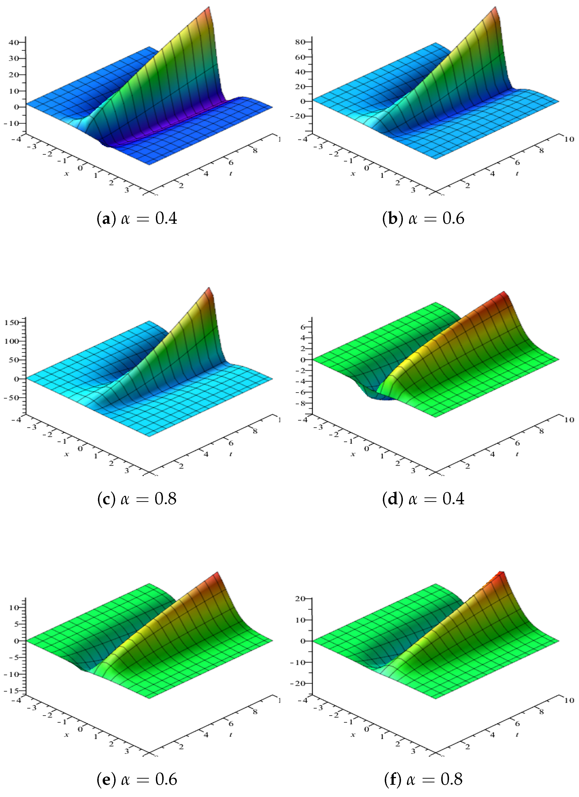
6. Numerical Simulation and Discussion

This section is dedicated to the presentation of the numerical simulations of q-homotopy analysis method (q-HAM) of Equation (1) [49]. The Equation (1) is taken as Caputo sense of $0<\alpha \le 1$.

Definition 3.

The fractional derivative in the Caputo’s sense is defined as [49]

$$D_t^{\alpha }f(t)=I^{m-\alpha }{D}^{n}f(t)=\frac{1}{\mathrm{\Gamma }(n-\alpha )}{\int }_0^t{(t-\tau )}^{n-\alpha -1}{f}^{(n)}(\tau )d\tau ,$$

(51)

where $n-1<\alpha \le n,n\in \mathbb{N},t>0$. For $\alpha =1$, the exact solutions of Equation (1) are given by [50]

$$\begin{array}{c}u(x,t)=\frac{ck}{2}+\frac{ck}{2}\tan \mathrm{h}(\frac{c{k}^{2}t-kx}{2}),\hfill \\ v(x,t)=-\frac{k^2}{8}{\sec \mathrm{h}}^2(\frac{kx-c{k}^{2}t}{2}).\hfill \end{array}$$

(52)

For simplicity, we choose special parameters $c=1$, $k=2$. Consider Equation (1) with initial conditions [50]

$$\begin{array}{c}u(x,t)=1-tanh(x),\hfill \\ v(x,t)=-\frac{1}{2}sec{h}^2(x).\hfill \end{array}$$

(53)

In order to get the series solution of Equation (1), we use the linear operators

$$\begin{array}{c}\mathfrak{L}[\phi (x,t;q)]=D_t^{\alpha }\phi (x,t;q),\hfill \\ \mathfrak{L}[\psi (x,t;q)]=D_t^{\alpha }\psi (x,t;q),\hfill \end{array}$$

(54)

with the specific property $\mathfrak{L}[r]=0$, where r is a constant. The nonlinear operators is defined as

$$\begin{array}{cc}\hfill \mathsf{\Phi }[\phi (x,t;q),\psi (x,t;q)]=& \frac{{\partial }^{\alpha }\phi (x,t;q)}{\partial t^{\alpha }}-\frac{1}{2}\psi (x,t;q)+2\phi (x,t;q)\frac{\partial \phi (x,t;q)}{\partial x},\hfill \\ \hfill \mathsf{\Phi }[\phi (x,t;q),\psi (x,t;q)]=& \frac{{\partial }^{\alpha }\psi (x,t;q)}{\partial t^{\alpha }}-\frac{1}{2}\frac{{\partial }^3\phi (x,t;q)}{\partial x^3}+2\phi (x,t;q)\frac{\partial \psi (x,t;q)}{\partial x}\hfill \\ & +2\psi (x,t;q)\frac{\partial \phi (x,t;q)}{\partial x}.\hfill \end{array}$$

(55)

Based on the theorem in [50], the nonlinear operators can be written as

$$\begin{array}{cc}\hfill \mathsf{\Phi }[\phi (x,t;q),\psi (x,t;q)]=& t^{1-\alpha }\frac{{\partial }^{\alpha }\phi (x,t;q)}{\partial t^{\alpha }}-\frac{1}{2}\frac{\psi (x,t;q)}{\partial x}+2\phi (x,t;q)\frac{\partial \phi (x,t;q)}{\partial x},\hfill \\ \hfill \mathsf{\Phi }[\phi (x,t;q),\psi (x,t;q)]=& t^{1-\alpha }\frac{{\partial }^{\alpha }\psi (x,t;q)}{\partial t^{\alpha }}-\frac{1}{2}\frac{{\partial }^3\phi (x,t;q)}{\partial x^3}+2\phi (x,t;q)\frac{\partial \psi (x,t;q)}{\partial x}\hfill \\ & +2\psi (x,t;q)\frac{\partial \phi (x,t;q)}{\partial x}.\hfill \end{array}$$

(56)

Therefore, the zero-order deformation equations are given by

$$\begin{array}{c}(1-nq)\mathfrak{L}[\phi (x,t;q)-u_0(x,t)]=qhM[\phi (x,t;q),\psi (x,t;q)],\hfill \\ (1-nq)\mathfrak{L}[\psi (x,t;q)-v_0(x,t)]=qhM[\phi (x,t;q),\psi (x,t;q)],\hfill \end{array}$$

(57)

choosing $M(x,t)=1$, the mth-order deformation equations can be given by

$$\begin{array}{c}\mathfrak{L}[u_m(x,t)-{\chi }_m^{*}{u}_{m-1}(x,t)]=h{R}_{m,1}({\mathbf{u}}_{m-1},{\mathbf{v}}_{m-1}),\hfill \\ \mathfrak{L}[v_m(x,t)-{\chi }_m^{*}{v}_{m-1}(x,t)]=h{R}_{m,2}({\mathbf{u}}_{m-1},{\mathbf{v}}_{m-1}),\hfill \end{array}$$

(58)

where

$$\begin{array}{c}\hfill {\chi }_m^{*}=\left\{\begin{array}{c}0,m\le 1,\hfill \\ n,otherwise,\hfill \end{array}\right.\end{array}$$

(59)

$$\begin{array}{cc}\hfill R_{m,1}({\mathbf{u}}_{m-1},{\mathbf{v}}_{m-1})=& t^{1-\alpha }\frac{\partial u_{m-1}(x,t)}{\partial t}-\frac{1}{2}\frac{\partial v_{m-1}(x,t)}{\partial x}+2\sum _{n=0}^{m-1}{u}_n(x,t)\frac{\partial u_{m-1-n}}{\partial x},\hfill \\ \hfill R_{m,2}({\mathbf{u}}_{m-1},{\mathbf{v}}_{m-1})=& t^{1-\alpha }\frac{\partial v_{m-1}(x,t)}{\partial t}-\frac{1}{2}\frac{{\partial }^3{u}_{m-1}(x,t)}{\partial x^3}+2\sum _{n=0}^{m-1}{u}_n(x,t)\frac{\partial v_{m-1-n}(x,t)}{\partial x}\hfill \\ & +2\sum _{n=0}^{m-1}{v}_n(x,t)\frac{\partial u_{m-1-n}(x,t)}{\partial x}.\hfill \end{array}$$

(60)

According to the simple transformation of Equation (58), we obtain

$$\begin{array}{c}{u}_m(x,t)={\chi }_m^{*}{u}_{m-1}(x,t)+h{\mathfrak{L}}^{-1}[R_{m,1}({\mathbf{u}}_{m-1},{\mathbf{v}}_{m-1})],\hfill \\ v_m(x,t)={\chi }_m^{*}{v}_{m-1}(x,t)+h{\mathfrak{L}}^{-1}[R_{m,2}({\mathbf{u}}_{m-1},{\mathbf{v}}_{m-1})].\hfill \end{array}$$

(61)

Thus we get the solutions

$$\begin{array}{c}{u}_1=(\frac{3}{2}sec{h}^2(x)tanh(x)-2sec{h}^2(x))\frac{h{t}^{\alpha }}{\mathrm{\Gamma }(1+\alpha )},\hfill \\ v_1=2sec{h}^2(x)tanh(x)\frac{h{t}^{\alpha }}{\mathrm{\Gamma }(1+\alpha )},\hfill \end{array}$$

(62)

and

$$\begin{array}{cc}\hfill u_2=& (\frac{3}{2}sec{h}^2(x)tanh(x)-2sec{h}^2(x))\frac{h(n+h)t^{\alpha }}{\mathrm{\Gamma }(1+\alpha )}+(-18sec{h}^2(x)tan{h}^2(x)\hfill \\ & +6sec{h}^2(x)+2sec{h}^2(x)tanh(x)+12tan{h}^3(x)sec{h}^2(x))\frac{h^2{t}^{2\alpha }}{\mathrm{\Gamma }(1+2\alpha )},\hfill \\ \hfill v_2=& 2sec{h}^2(x)tanh(x)\frac{h(n+h)t^{\alpha }}{\mathrm{\Gamma }(1+\alpha )}+(10sec{h}^2(x)-57sec{h}^2(x)tan{h}^2(x)\hfill \\ & +45sec{h}^2(x)tan{h}^4(x)+8sec{h}^2(x)tanh(x)-8sec{h}^2(x)tan{h}^3(x)\hfill \\ & +\frac{15}{2}sec{h}^4(x)tan{h}^2(x)-8sec{h}^4(x)tanh(x)-\frac{3}{2}sec{h}^4(x))\frac{h^2{t}^{2\alpha }}{\mathrm{\Gamma }(1+2\alpha )}.\hfill \end{array}$$

(63)

In the same way, $u_m(x,t),v_m(x,t)$ for $m=3,4,5,\cdots$ can be obtained by using Maple. Then the series solution expression by q-HAM can be written as follows

$$\begin{array}{c}u(x,t;n;h)=1-tanh(x)+\sum _{i=1}^{\infty }{u}_i(x,t;n;h){(\frac{1}{n})}^i,\hfill \\ v(x,t;n;h)=-\frac{1}{2}sec{h}^2(x)+\sum _{i=1}^{\infty }{v}_i(x,t;n;h){(\frac{1}{n})}^i,\hfill \end{array}$$

(64)

u and v are appropriate solutions to the problem Equation (1) in terms of convergence parameter h and n. Now we give numerical results to prove the effectiveness of q-HAM. The following figure shows the q-HAM and exact solutions of Equation (1) for different values of α.

Remark 1.

Using the first two terms of the q-HAM series in Equation (64), when $n=2$, we choose appropriate $h=1$ to get

$$\begin{array}{c}u(x,t;n;h)=1-tanh(x)+(\frac{3}{2}sec{h}^2(x)tanh(x)-2sec{h}^2(x))\frac{4t^{\alpha }}{\mathrm{\Gamma }(1+\alpha )},\hfill \\ v(x,t;n;h)=-\frac{1}{2}sec{h}^2(x)+8sec{h}^2(x)tanh(x)\frac{t^{\alpha }}{\mathrm{\Gamma }(1+\alpha )}.\hfill \end{array}$$

(65)

Thus, we get exact solution to the Equation (1) given by just two terms of the series.

Remark 2.

Figure 2 displays the solution plot of the coupled time-fractional Boussinesq-Burgers system obtained by the q-HAM, while Figure 3 displays the exact solutions for the same equation when $\alpha =0.4$, $\alpha =0.6$, $\alpha =0.8$, respectively. It should be noted that only three terms of the q-HAM series solution are used for the plot. The results match comparatively with results of other analytical methods. It is easy to observe that the amplitude of u and v increase with the increase of α.

7. Conclusions

In this paper, the fractional Lie symmetry analysis to the coupled time-fractional Boussinesq-Burgers system has been performed. Based on the fractional Lie symmetry analysis approach, we have determined vector fields and reduced it to the system of FODEs. We have solved the reduced system of FODEs by using the power series expansion method. Meanwhile, the convergence of power series solution is analyzed. Especially, by using the new conservation theorem, the conservation laws of Equation (1) have also been constructed on the basis of the obtained symmetries. Finally, the approximate analytical solution was studied by employing the q-homotopy analysis method under the background of Caputo fractional differential. This method has achieved good results in practical application and could be easily applied to fractional fluid problem such as the Boussinesq-Burgers system and other fractional order nonlinear evaluation problems.

References

1. Vinagre, B.M.; Podlubny, I.; Hernandez, A.; Feliu, V. Some approximations of fractional order operators used in control theory and applications. Fract. Calc. Appl. Anal. 2000, 3, 231–248. [Google Scholar]
2. Oldham, K.; Spanier, J. The Fractional Calculus Theory and Applications of Differentiation and Integration to Arbitrary Order; Elsevier: Amsterdam, The Netherlands, 1974. [Google Scholar]
3. Samko, S.G.; Kilbas, A.A.; Marichev, O.I. Fractional Integrals and Derivatives: Theory and Applications; Gordon and Breach Science Publishers: Philadelphia, PA, USA, 1993; pp. 397–414. [Google Scholar]
4. Tchier, F.; Yusuf, A.; Aliyu, A.I.; Baleanu, D. Time fractional third-order variant Boussinesq system: Symmetry analysis, explicit solutions, conservation laws and numerical approximations. Eur. Phys. J. Plus 2018, 133, 240. [Google Scholar] [CrossRef]
5. Gazizov, R.K.; Kasatkin, A.A.; Lukashchuk, S.Y. Continuous transformation groups of fractional differential equations. Vestnik Usatu 2007, 9, 21. [Google Scholar]
6. Sahadevan, R.; Bakkyaraj, T. Invariant analysis of time fractional generalized Burgers and Korteweg-de Vries equations. J. Math. Anal. Appl. 2012, 393, 341–347. [Google Scholar] [CrossRef]
7. Gazizov, R.K.; Kasatkin, A.A.; Lukashchuk, S.Y. Symmetry properties of fractional diffusion equations. Phys. Scr. 2009, 2009, 014016. [Google Scholar] [CrossRef]
8. Buckwar, E.; Luchko, Y. Invariance of a partial differential equation of fractional order under the Lie group of scaling transformations. J. Math. Anal. Appl. 1998, 227, 81–97. [Google Scholar] [CrossRef]
9. Bakkyaraj, T.; Sahadevan, R. Invariant analysis of nonlinear fractional ordinary differential equations with Riemann-Liouville fractional derivative. Nonlinear Dyn. 2015, 80, 447–455. [Google Scholar] [CrossRef]
10. Ouhadan, A.; Elkinani, E.H. Exact solutions of time fractional Kolmogorov equation by using Lie symmetry analysis. J. Fract. Calc. Appl. 2014, 5, 97–104. [Google Scholar]
11. Wang, G.; Liu, X.; Zhang, Y. Lie symmetry analysis to the time fractional generalized fifth-order KdV equation. Commun. Nonlinear Sci. Numer. Simul. 2013, 18, 2321–2326. [Google Scholar] [CrossRef]
12. Wang, X.B.; Tian, S.F.; Qin, C.Y.; Zhang, T.T. Lie symmetry analysis, conservation laws and exact solutions of the generalized time fractional Burgers equation. Europhys. Lett. 2016, 114, 20003. [Google Scholar] [CrossRef]
13. Jannelli, A.; Ruggieri, M.; Speciale, M.P. Exact and numerical solutions of time-fractional advection-diffusion equation with a nonlinear source term by means of the Lie symmetries. Nonlinear Dyn. 2018, 92, 543–555. [Google Scholar] [CrossRef]
14. Hosseini, V.R.; Shivanian, E.; Chen, W. Local integration of 2-D fractional telegraph equation via local radial point interpolant approximation. Eur. Phys. J. Plus 2015, 130, 33. [Google Scholar] [CrossRef]
15. Rui, W.; Zhang, X. Invariant analysis and conservation laws for the time fractional foam drainage equation. Eur. Phys. J. Plus 2015, 130, 192. [Google Scholar] [CrossRef]
16. Wang, G.; Kara, A.H.; Fakhar, K. Symmetry analysis and conservation laws for the class of time-fractional nonlinear dispersive equation. Nonlinear Dyn. 2015, 82, 281–287. [Google Scholar] [CrossRef]
17. Cao, J.; Syta, A.; Litak, G.; Zhou, S.; Inman, D.J.; Chen, Y. Regular and chaotic vibration in a piezoelectric energy harvester with fractional damping. Eur. Phys. J. Plus 2015, 130, 103. [Google Scholar] [CrossRef] [Green Version]
18. Wang, G.W.; Xu, T.Z. Invariant analysis and exact solutions of nonlinear time fractional Sharma-Tasso-Olver equation by Lie group analysis. Nonlinear Dyn. 2014, 76, 571–580. [Google Scholar] [CrossRef]
19. Zhang, Y.; Mei, J.; Zhang, X. Symmetry properties and explicit solutions of some nonlinear differential and fractional equations. Appl. Math. Comput. 2018, 337, 408–418. [Google Scholar] [CrossRef]
20. Qin, C.Y.; Tian, S.F.; Wang, X.B.; Zhang, T.T. Lie symmetries, conservation laws and explicit solutions for time fractional Rosenau-Haynam equation. Commun. Theor. Phys. 2017, 67, 157. [Google Scholar] [CrossRef]
21. Singla, K.; Gupta, R.K. On invariant analysis of some time fractional nonlinear systems of partial differential equations. J. Math. Phys. 2016, 57, 101504. [Google Scholar] [CrossRef]
22. Singla, K.; Gupta, R.K. Conservation laws for certain time fractional nonlinear systems of partial differential equations. Commun. Nonlinear Sci. Numer. Simul. 2017, 53, 10–21. [Google Scholar] [CrossRef]
23. Noether, E. Invariant variation problems. Transp. Theory Stat. Phys. 1971, 1, 186–207. [Google Scholar] [CrossRef] [Green Version]
24. Lukashchuk, S.Y. Conservation laws for time-fractional subdiffusion and diffusion-wave equations. Nonlinear Dyn. 2015, 80, 791–802. [Google Scholar] [CrossRef] [Green Version]
25. Ibragimov, N.H. A new conservation theorem. J. Math. Anal. Appl. 2007, 333, 311–328. [Google Scholar] [CrossRef] [Green Version]
26. Khater, M.M.A.; Kumar, D. New exact solutions for the time fractional coupled Boussinesq-Burger equation and approximate long water wave equation in shallow water. J. Ocean Eng. Sci. 2017, 2, 223–228. [Google Scholar] [CrossRef]
27. Yang, X.J.; Baleanu, D.; Srivastava, H.M. Local Fractional Integral Transforms and Their Applications; Academic Press: Cambridge, MA, USA, 2015. [Google Scholar]
28. Yang, X.J.; Srivastava, H.M.; Machado, J.A. A new fractional derivative without singular kernel: Application to the modelling of the steady heat flow. arXiv, 2015; arXiv:1601.01623. [Google Scholar] [CrossRef]
29. Liao, H.; Lyu, P.; Vong, S. Second-order BDF time approximation for Riesz space-fractional diffusion equations. Int. J. Comput. Math. 2018, 95, 1–18. [Google Scholar] [CrossRef]
30. Zhang, S. Monotone iterative method for initial value problem involving Riemann-Liouville fractional derivatives. Nonlinear Anal. Theory Methods Appl. 2009, 71, 2087–2093. [Google Scholar] [CrossRef]
31. Agarwal, R.P.; Belmekki, M.; Benchohra, M. A survey on semilinear differential equations and inclusions involving Riemann-Liouville fractional derivative. Adv. Differ. Equ. 2009, 2009, 981728. [Google Scholar] [CrossRef]
32. Heymans, N.; Podlubny, I. Physical interpretation of initial conditions for fractional differential equations with Riemann-Liouville fractional derivatives. Rheol. Acta 2006, 45, 765–771. [Google Scholar] [CrossRef]
33. He, J.H. Approximate analytical solution for seepage flow with fractional derivatives in porous media. Comput. Methods Appl. Mech. Eng. 1998, 167, 57–68. [Google Scholar] [CrossRef]
34. Agrawal, O.P. Formulation of Euler-Lagrange equations for fractional variational problems. J. Math. Anal. Appl. 2002, 272, 368–379. [Google Scholar] [CrossRef]
35. Deng, W.; Li, C.; Lü, J. Stability analysis of linear fractional differential system with multiple time delays. Nonlinear Dyn. 2007, 48, 409–416. [Google Scholar] [CrossRef]
36. Frederico, G.S.F.; Torres, D.F.M. Fractional conservation laws in optimal control theory. Nonlinear Dyn. 2008, 53, 215–222. [Google Scholar] [CrossRef]
37. Jumarie, G. Table of some basic fractional calculus formulae derived from a modified Riemann-Liouville derivative for non-differentiable functions. Appl. Math. Lett. 2009, 22, 378–385. [Google Scholar] [CrossRef]
38. Jumarie, G. Laplace’s transform of fractional order via the Mittag-Leffler function and modified Riemann-Liouville derivative. Appl. Math. Lett. 2009, 22, 1659–1664. [Google Scholar] [CrossRef]
39. Singla, K.; Gupta, R.K. Space-time fractional nonlinear partial differential equations: symmetry analysis and conservation laws. Nonlinear Dyn. 2017, 89, 321–331. [Google Scholar] [CrossRef]
40. Kilbas, A.A.; Srivastava, H.M.; Trujillo, J.J. Theory and Applications of Fractional Differential Equations; Elsevier: San Diego, CA, USA, 2006. [Google Scholar]
41. Miller, K.S.; Ross, B. An Introduction to the Fractional Calculus and Fractional Differential Equations; Wiley-Interscience: Hoboken, NJ, USA, 1993. [Google Scholar]
42. Podlubny, I. Fractional Differential Equations: An Introduction to Fractional Derivatives, Fractional Differential Equations, to Methods of Their Solution and Some of Their Applications; Elsevier: San Diego, CA, USA, 1998. [Google Scholar]
43. Huang, H.N.; Marcantognini, S.A.M.; Young, N.J. Chain rules for higher derivatives. Math. Intell. 2006, 28, 61–69. [Google Scholar] [CrossRef] [Green Version]
44. Leo, R.A.; Sicuro, G.; Tempesta, P. A foundational approach to the Lie theory for fractional order partial differential equations. Fract. Calc. Appl. Anal. 2017, 20, 212–231. [Google Scholar] [CrossRef]
45. Kiryakova, V.S. Generalized Fractional Calculus and Applications; CRC Press: Boca Raton, FL, USA, 1993. [Google Scholar]
46. Mathai, A.M.; Haubold, H.J. Erdélyi-Kober fractional integral operators from a statistical perspective. Tbilisi Math. J. 2017, 10, 145–159. [Google Scholar] [CrossRef]
47. Sneddon, I.N. The use in mathematical physics of Erdélyi-Kober operators and of some of their generalizations. In Fractional Calculus and Its Applications; Springer: Berlin/Heidelberg, Germany, 1975; pp. 37–79. [Google Scholar]
48. Rudin, W. Principles of Mathematical Analysis; McGraw-hill: New York, NY, USA, 1976. [Google Scholar]
49. Iyiola, O.S.; Olayinka, O.G. Analytical solutions of time-fractional models for homogeneous Gardner equation and non-homogeneous differential equations. Ain Shams Eng. J. 2014, 5, 999–1004. [Google Scholar] [CrossRef] [Green Version]
50. He, J.H. Homotopy perturbation method: A new nonlinear analytical technique. Appl. Math. Comput. 2003, 135, 73–79. [Google Scholar] [CrossRef]
Figure 1. Panels (a,b) represent the 3-dimensional plots for u ( x , t ) with a 0 = a 1 = a 2 = b 0 = b 1 = b 2 = 1 . Panels (c,d) represent the 3-dimensional plots for v ( x , t ) with a 0 = a 1 = a 2 = b 0 = 1 .
Symmetry 11 00077 g001
Figure 2. Profiles of the q-HAM series solution for the Equation (1) with the same parameters α = 0 . 4 , α = 0 . 6 , α = 0 . 8 , respectively. (ac) three dimensional plot of u. (df) three dimensional plot of v.
Symmetry 11 00077 g002
Figure 3. Profiles of the exact solution for the Equation (1) with the same parameters α = 0 . 4 , α = 0 . 6 , α = 0 . 8 , respectively. (ac) three dimensional plot of u. (df) three dimensional plot of v.
Symmetry 11 00077 g003