Volumes of Hyperbolic Three-Manifolds Associated with Modular Links

Abstract

Periodic geodesics on the modular surface correspond to periodic orbits of the geodesic flow in its unit tangent bundle ${\mathrm{PSL}}_2(\mathbb{Z})\backslash {\mathrm{PSL}}_2(\mathbb{R})$. A finite collection of such orbits is a collection of disjoint closed curves in a 3-manifold, in other words a link. The complement of those links is always a hyperbolic 3-manifold, and hence has a well-defined volume. We present strong numerical evidence that, in the case of the set of geodesics corresponding to the ideal class group of a real quadratic field, the volume has linear asymptotics in terms of the total length of the geodesics. This is not the case for general sets of geodesics.

1. Introduction

Let X be a three-dimensional manifold. A knot in X is a simple closed smooth curve, considered up to deformation; a link in X is a collection of such pairwise disjoint curves, again considered up to deformation.

We study numerically the topological type of knots and links arising from closed geodesics on the modular surface. These geodesics have number-theoretic meaning, and we show evidence of an interesting behaviour for the links that arise when the geodesics are grouped in a number-theoretic relevant way.

In the rest of this introduction, we review these general ideas, discuss the motivation for our work, and outline the rest of the paper.

1.1. Knots Associated with Closed Geodesics

Let M be a Riemannian surface, that is, a surface equipped with a Riemannian metric. Its unit tangent bundle is the bundle whose fibre over every $p\in M$ is the circle of direction vectors at p. We note that this bundle (denoted $T^{1}M$) is a three-dimensional manifold.

Now, let $\gamma :[a,b]\to M$ be a smooth closed curve on M, parametrized to have unit speed (smoothness at the endpoints requires not merely that $\gamma (a)=\gamma (b)$ but that the derivatives match to all orders). Then, for every $t\in [a,b]$, the derivative $\dot{\gamma }(t)$ is a unit (=direction) vector at $\gamma (t)\in M$, so that the map $t\mapsto \left(\gamma (t),\dot{\gamma }(t)\right)$ describes a closed curve in $T^{1}M$. We require the self-intersection of the curve to be transverse (the direction vectors must be distinct) so that the lift to $T^{1}M$ is not self-intersecting. Included in this is the assumption that the curve is primitive (not a power of another curve). For such a curve, the (smooth) isotopy class of its lift in $T^{1}M$ is a knot therein.

Moreover, any smooth deformation of $\gamma$ into a curve ${\gamma }^{\prime }$ can be modified to preserve the unit speed parametrization, at which point it can be lifted to a deformation of the lifted curves in $T^{1}M$. In other words, the resulting knots depend only on the deformation (isotopy) class of the curve. In addition, we may construct a link by beginning with several curves as long as all intersections (including self-intersections) are transverse.

Changing the metric on M does not affect the topological properties of $T^{1}M$ or the embeddings on curves, so (excluding the sphere and the torus, which we do from now on) we may equip our surface with a finite-volume metric of constant negative curvature −1; that is, we realize it as a hyperbolic surface (for the geometry of such surfaces see [1]). Fixing such a metric, each isotopy class of primitive closed curves is one of two types. Generically, such a class contains a unique representative of shortest length, necessarily a closed geodesic. If the surface is non-compact and hence has cusps (infinitely long asymptotically narrow ends), there are also finitely many classes of “periodic horocycles”, curves going around a cusp. Curves in the latter class can be deformed to be arbitrarily short by “sliding them off the cusp” toward infinity.

1.2. Modular Links and Their Volumes

One specific non-compact hyperbolic surface is the modular surface reviewed in Section 2. Remarkably, this surface, its unit tangent bundle and its closed geodesics have explicit realizations.

The recent surge of interest in “modular links”, that is, those that arise from lifting closed geodesics on the modular surface, stems from the work of Ghys [2], where the closed geodesics were connected to the periodic orbits of the Lorentz attractor, a classical example of a chaotic dynamical system.

Furthermore, there is a natural embedding of the unit tangent bundle of the modular surface as the complement of a specific knot (the trefoil) in the three-dimensional sphere. Via this embedding, we augment each modular knot or link to a link in the three-sphere with an additional component (this trefoil knot). Ghys showed that the linking number of each modular knot with the trefoil can be computed via the Rademacher function, a classical function on the modular group ${\mathrm{SL}}_2(\mathbb{Z})$, and this allowed Sarnak [3] to count geodesics by linking number.

Our contribution here is to study the topology of the augmented links directly, specifically through properties of their complements. Note that the complement of the augmented link in the three-sphere is exactly the complement of the original link in the unit tangent bundle. For the purposes of exposition, it is more convenient to consider the complements in the form $X\backslash \gamma$ where X is the unit tangent bundle of the modular surface and $\gamma$ is the (lift) of a family of closed geodesics, while, for computational purposes, it will be convenient to include the trefoil component in the calculations.

The starting point of our study is the fact that our link complements $X\backslash \gamma$ always have a hyperbolic structure—they can be endowed with a finite-volume complete Riemann metric of constant curvature $-1$ (for a proof, see [4]). By Mostow’s Strong Rigidity Theorem, this hyperbolic structure is unique, so that metric properties of the resulting Riemannian 3-manifold are in fact topological properties of the link, depending only on the deformation class of the curves making up $\gamma$.

We focus here on the simplest invariant of a hyperbolic three-manifold, its volume, and specifically study the relationship between the volume of $X\backslash \gamma$ and the complexity of $\gamma$ as measured by the total length of its constituent geodesics (from the topological point of view, we essentially defined the length of a curve by taking the length of the shortest representative in its deformation class). Following the usual convention in topology, we shorten “the volume of the complement of $\gamma$” to “the volume of $\gamma$”.

In the related work sharing several authors [5], we have shown that there is a universal constant C such that the volume of a modular link is bounded by C times its length. While a matching lower bound is not possible in general (see Examples 1 and 2 below), it is nevertheless interesting to ask if our bound is sharp, that is, if there are some links whose volumes grow linearly with their length. Experimentally, this seems to be the case for the links considered here.

1.3. Results and Structure of This Paper

Specifically, for each square-free positive integer $d>1$, let ${\gamma }_d$ be the set of geodesics corresponding to the ideal classes in the ring of integers of the quadratic field $\mathbb{Q}(\sqrt{d})$ (for details, see Section 2). It is a beautiful theorem of Duke [6] that these sets of geodesics are becoming uniformly distributed on X: for any compactly supported continuous function f on X, the averages of f on the geodesics in ${\gamma }_d$ (with respect to the length measure) converge to the average of f on X (with respect to its Riemannian volume). Inspired by this, we examine numerically the volume of the complements of these sets.

In Section 2, we discuss the modular surface, its unit tangent bundle, and the relationship between lifts of closed geodesics there and equivalence classes of integral binary quadratic forms and construct the so-called “fundamental” geodesics, those associated with the ideal classes in the ring of integers of a real quadratic field, equivalently to classes of quadratic forms of fundamental discriminant.

In Section 3, we review the passage from number theory to topology: the coding of geodesics by positive words in the two-letter alphabet $\{X,Y\}$, how to obtain the coding of a geodesic from the corresponding quadratic form, as well as Williams’s algorithm giving a combinatorial description of the resulting link in X from the list of words.

We use SageMath [7] and SnapPy [8] to numerically obtain the volume of the complement from this combinatorial description; we give the details in Section 4.

Finally, in Section 5, we present our main result for the family of links corresponding to the class groups of the fields $\mathbb{Q}\left(\sqrt{d}\right)$ with d ranging over the square-free numbers up to 1000 (608 fields), the volumes seem to lie very close to the best-fit line

$$\mathrm{volume}\approx 3.24\ast \mathrm{length}+0.01.$$

2. Modular Links and Quadratic Fields

2.1. Periodic Geodesics on the Modular Surface

Let $G={\mathrm{PSL}}_2(\mathbb{R})={\mathrm{SL}}_2(\mathbb{R})/\left\{\pm I\right\}$ be the quotient of the unimodular group ${\mathrm{SL}}_2(\mathbb{R})$ by its centre. G acts on the upper half-plane $\mathbb{H}=\{z=x+iy\mid y>0\}$ via the fractional linear transformations

$$\left(\begin{array}{cc}a& b\\ c& d\end{array}\right)·z=\frac{az+b}{cz+d}.$$

The action is transitive and the stabilizer of i is the circle group $K=\mathrm{SO}(2)$, so that $\mathbb{H}=G/K$.

The G action on $\mathbb{H}$ preserves the Riemannian metric $d{s}^2=\frac{d{x}^2+d{y}^2}{y^2}$, of constant negative curvature $-1$, giving a realization of the hyperbolic plane. The circle bundle $G\to \mathbb{H}$ is exactly the unit tangent bundle. Concretely, the Gram–Schmidt decomposition of $g\in G$ (or Iwasawa decomposition) takes the form

$$g=\left(\begin{array}{cc}1& x\\ & 1\end{array}\right)\left(\begin{array}{cc}{y}^{1/2}& \\ & y^{-1/2}\end{array}\right)\left(\begin{array}{cc}cos(\theta /2)& sin(\theta /2)\\ -sin(\theta /2)& cos(\theta /2)\end{array}\right),$$

which we interpret as the tangent vector in direction $\theta$ at the point $z=x+iy\in \mathbb{H}$ ($\theta =0$ corresponds to vectors pointing directly upward in the half-plane realization above).

The geodesic flow on the tangent bundle is the flow where the vector $(z,\theta )$ flows along the geodesic starting at z in the direction $\theta$—in terms of our representation, above moving distance t along the geodesic amounts to multiplying $g=(z,\theta )$ on the right by $a_t=\left(\begin{array}{cc}{e}^{t/2}& 0\\ 0& e^{-t/2}\end{array}\right)$.

Now, let $\Gamma ={\mathrm{PSL}}_2(\mathbb{Z})$, a discrete subgroup of G. The quotient $M=\Gamma \backslash \mathbb{H}$ is the celebrated modular surface. Its points parametrize, for example, lattices in ${\mathbb{R}}^2$ up to rotation and scaling. Furthermore, the quotient space $X=\Gamma \backslash G$ is clearly the unit tangent bundle of M. Geodesic flow on $X=T^{1}M$ is still given by the right action of $A={\{a_t\}}_{t\in \mathbb{R}}$.

Remark 1.

Since Γ has elements of finite orders, the quotient M is formally an orbifold rather than a manifold. This distinction, however, is irrelevant to the discussions here. These elements of finite order will play a role in Section 3.

In the realization X of the tangent bundle, the geodesic through the coset $x=\Gamma g\in X$ is periodic if and only if we have some non-identity $a_t\in A$ such that $x·a_t=x$, equivalently such that $g·a_t=\gamma g$. Rewriting this as $g^{-1}\gamma g=a_t$, we see that a closed geodesic is determined by a matrix $\gamma \in \Gamma$ having distinct real eigenvalues. It is easy to check that conjugating $\gamma$ by $\eta \in \Gamma$ amounts to replacing g with $\eta g$, so that periodic geodesics are in bijection with conjugacy classes in $\Gamma$ of elements diagonalizable over $\mathbb{R}$. We also need to restrict to $\gamma$ what are not proper powers of other elements of $\Gamma$ (“primitive” conjugacy classes) since powers amount to geodesics going around the same loop multiple times.

For simplicity, we shall use $\gamma$ to interchangeably denote the closed geodesic on M, its lift to X, the corresponding primitive conjugacy class in $\Gamma$ or a representative element of the conjugacy class.

2.2. Quadratic Forms and Geodesics

Each geodesic on M is the projection to M of a geodesic in $\mathbb{H}$, and such geodesics can be infinitely extended to have two endpoints on the circle at infinity (this is similar to the case of straight lines in the flat plane). In the upper half-plane model, the circle at infinity consists of the real line (the obvious boundary of the upper half-plane) and a single point thought of as lying at imaginary infinity. The geodesics accordingly take one of two forms: either both of the endpoints lie on the real axis, and then the geodesic is the Euclidean semicircle whose diameter is the interval between the two endpoints, or one endpoint is at infinity, and then the geodesic is the vertical line touching the other endpoint.

In particular, a geodesic not passing through $i\infty$ can be encoded by the quadratic polynomial whose roots are the two endpoints, equivalently by any quadratic form $q(x,y)=a{x}^2+bxy+c{y}^2$ such that the endpoints are the roots of the polynomial $a{z}^2+bz+c$ (this is unique up to scaling).

It is well known that the projection to M of a geodesic is periodic exactly when its endpoints are conjugate quadratic irrationalities, or, equivalently, when the quadratic form can be taken to have integral coefficients, and we now study those.

An integral binary quadratic form is the homogenous polynomial $q(x,y)=a{x}^2+bxy+c{y}^2$ with $a,b,c\in \mathbb{Z}$. Its discriminant is the quantity $d=b^2-4ac$, and we will only consider the indefinite case where $d>0$. Accordingly, we will shorten the “indefinite integral binary quadratic form” to “quadratic form”.

We give below a formula of a matrix $\gamma \in \Gamma$ representing the conjugacy class corresponding to the geodesic determined by a quadratic form q.

Now, $\Gamma$ acts on the set of quadratic forms by composition: thinking of a quadratic form q as a function on ${\mathbb{Z}}^2$, for any $\eta \in \Gamma$, the composition $q\circ {\eta }^{-1}$ is another such function that is another quadratic form. The orbits are called equivalence classes or simply classes of quadratic forms. It is easy to verify that replacing q with $q\circ {\eta }^{-1}$ replaces the points $z_1,z_2$ with $\eta ·z_1,\eta ·z_2$ and hence translates the geodesic connecting them by $\eta$. In particular, classes of quadratic forms correspond to geodesics in the quotient $\Gamma \backslash \mathbb{H}$, and the result is a bijection between classes of quadratic forms and periodic geodesics.

We do not know much about the way in which topological properties of geodesics as knots, and their algebraic properties as elements in this groups interact via this correspondence. This has been studied in [9], and we hope the current work makes a case for further study.

It is easy to check that equivalent forms have the same discriminant. It was shown by Gauss that, for each $d\ne 0$, there are finitely many equivalence classes having discriminant d (we concentrate on $d>0$).

It is useful to consider yet another number-theoretic description: each class of quadratic forms with discriminant d corresponds to a class of invertible ideals in the quadratic order of discriminant d (see, for example, the book [10], which develops the theory of quadratic fields through this correspondence, which is the historical point of view). In the particular case of fundamental discriminants (those which are discriminants of quadratic fields), the correspondence is with ideals classes in the ring of integers of the corresponding field and we give one direction of the correspondence: the subring ${\mathcal{O}}_d=Z\left[\frac{d+\sqrt{d}}{2}\right]$ of the field $K=\mathbb{Q}\left(\sqrt{d}\right)$ is its ring of integers. Every ideal $\mathfrak{a}⊲{\mathcal{O}}_d$ is a free $\mathbb{Z}$-module of rank 2. Restricting the norm form $N_{\mathbb{Q}}^K$ to $\mathfrak{a}$ therefore gives an integral quadratic form. Furthermore, equivalent ideals (those that differ by an element of $K^{\times }$) correspond to equivalent quadratic forms, giving a bijection between the group of ideal classes and the set of classes of quadratic forms.

The group ${\mathcal{O}}_d^{\times }$ of units (invertible elements) of the ring ${\mathcal{O}}_d$ always has the form ${\left\{\pm {ϵ}^j\right\}}_{j\in \mathbb{Z}}$, and we call $ϵ$ a fundamental unit (there are four such elements, but choosing any of them will give the same results).

Letting m denote the square free part of d, we have $K=\mathbb{Q}\left(\sqrt{m}\right)$, and we represent each element of K in the form $x+\sqrt{m}y$. Then, ${\mathcal{O}}_d$ contains the elements of this form with $x,y\in \mathbb{Z}$ but may also contain those elements where $x,y$ are both half-integers (elements in $\mathbb{Z}+\frac{1}{2}$), the latter case occurring exactly when $m\equiv 1(4)$. In this latter case, we have $d=m$, and otherwise $d=4m$.

3. Coding of Geodesics

3.1. Conjugacy Classes in ${\mathrm{PSL}}_2(\mathbb{Z})$ and Words in Two Generators

Continuing with our previous conventions, we represent elements of ${\mathrm{PSL}}_2(\mathbb{Z})$ by preimages in ${\mathrm{SL}}_2(\mathbb{Z})$. Specifically, let $U=\left(\begin{array}{cc}0& 1\\ -1& 0\end{array}\right)$ and $V=\left(\begin{array}{cc}0& -1\\ 1& 1\end{array}\right)$. It is not hard to check that $U,V\in {\mathrm{PSL}}_2(\mathbb{Z})$ are elements of order $2,3$, respectively, and it is well-known that ${\mathrm{PSL}}_2(\mathbb{Z})$ is the free product of the cyclic groups generated by U and V. Accordingly, every element of the group has a unique representation as a reduced word in $U,V$ that is a word in this alphabet containing no subword of the form $UU$ or $VVV$ (note that only positive words are necessary since $U^{-1}=U$ and $V^{-1}=V^2$).

Recalling that periodic geodesics correspond to (certain) conjugacy classes in ${\mathrm{PSL}}_2(\mathbb{Z})$, we now discuss canonical representatives for those. Note that, if a word begins and ends in U, then it can be thought of as beginning with U and ending with $U^{-1}=U$, thus deleting the Us at the ends doesn’t affect the conjugacy class. Similarly, if the words beings with V or $V^2$, one can conjugate by $V^2$ or V to obtain a word beginning with U. The elements of finite order in ${\mathrm{PSL}}_2(\mathbb{Z})$ are exactly those conjugate to $1,U,V,V^2$, and we see that every conjugacy class of elements of infinite order contains a shortest representative, which is a positive word in the alphabet $X,Y$ where $X=UV$, $Y=U{V}^2$. Note that $X=\left(\begin{array}{cc}1& 1\\ 0& 1\end{array}\right)$ and $Y=\left(\begin{array}{cc}1& 0\\ 1& 1\end{array}\right)$.

The shortest representative of the conjugacy class is unique (as a word in $U,V$) up to cyclic permutation (this is a general fact about free products). It follows that every conjugacy class of elements of infinite order has a representative as a word in $X,Y$, unique up to cyclic permutation. We also know that an element of ${\mathrm{PSL}}_2(\mathbb{Z})$ is a power of another if and only if the corresponding word in $X,Y$ is periodic, so that primitive conjugacy classes correspond to primitive words (those that don’t consist of repetitions of a subword). We also note that every parabolic element of ${\mathrm{PSL}}_2(\mathbb{Z})$ is conjugate to a power of X (possibly negative). Since Y is conjugate to $X^{-1}$, we see that the words of the form $X^k$ or $Y^k$ ($k\ge 1$) exactly parametrize the parabolic conjugacy classes.

Conclusion: primitive closed geodesics on the modular surface are in bijection with positive words in $X,Y$ containing both symbols.

3.2. From Matrices to Words

For sake of completeness, we mention the algorithmic solution to obtaining the word in the generators $X,Y$, given the matrix representation of a hyperbolic element of ${\mathrm{PSL}}_2(\mathbb{Z})$.

Given a matrix $A=\left(\begin{array}{cc}a& b\\ c& d\end{array}\right)\in {\mathrm{PSL}}_2(\mathbb{Z})$, we first represent A as a product of U and $X=UV$, as follows: multiplying any matrix A by U will switch its first and second rows, and multiply the second row by $-1$. Next, multiplying by ${(UV)}^n$ will add n times the second row to the first. Thus, we may assume that $|a|\ge |c|$ by multiplying by U if needed. We may also assume that a is positive as $A\equiv -A$. Then, we can subtract n times $|c|$ from a, for the largest n such that $a-nc\ge 0$. Continuing in this way, we are actually applying the Euclidean algorithm to a and c. As $det(A)=ad-bc=1$, a and c are relatively prime, and thus, in a finite number of steps, we reach a matrix $A^{\prime }=\left(\begin{array}{cc}1& 0\\ c& d\end{array}\right)$. However, as $A^{\prime }\in {\mathrm{PSL}}_2(\mathbb{Z})$ $d=1$, and so $A^{\prime }={(UV)}^m$ for some integer $m\ne 0$. This results in a decomposition of A into the generators U and V. By switching to positive powers and grouping the generators into subsequences of $UV$ and $U{V}^2$, we reach the desired representation.

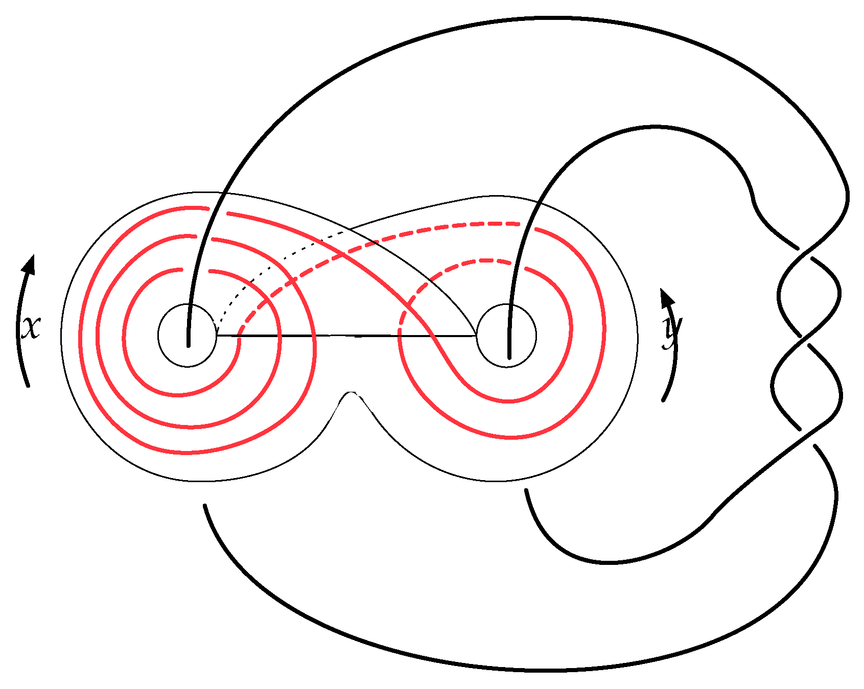
3.3. Curves from Words and the Template

In order to investigate the topology of the closed geodesics, we need a way to explicitly construct a representative of the isotopy class of the geodesic on the unit tangent bundle from a representation of the conjugacy class. This was done by Ghys [2], as follows.

A template [11] is a branched surface with boundary and an expansive semi flow. The following is a theorem of Ghys, relying on a theorem of Birman and Williams [11], which asserts that any Anosov flow on a three manifold has a template.

Theorem 1

(Ghys, [2]). The set of periodic geodesics on M is in bijective correspondence with the set of periodic orbits on the template T embedded in $S^3\backslash \mathit{trefoil}$ as depicted in Figure 1, excluding the boundary curves of T. On any finite subset, the correspondence is by an ambient isotopy.

This means that, in order to study knot properties of closed modular geodesics, one may study closed orbits on the template T. The template comes with a symbolic dynamics given by the symbols x and y that correspond to passing through the left or through the right ear (or equivalently through the left or the right half of the branch line, which is a Birkhoff section for the semiflow). Ghys proves in [2] that the symbolic dynamics of the representation of a geodesic in T is equivalent to its representation as a word in the generators $X,Y$ for ${\mathrm{PSL}}_2(\mathbb{Z})$.

4. Computational Method

We start with some table of quadratic fields and generate the matrices as explained in Section 3.1.

To decompose a matrix into a product of X and Y, we use a standard algorithm to decompose matrices in $S{L}_2(\mathbb{Z})$.

Then, given the corresponding periodic words in $x,y$, Williams [12] provides an algorithm for locating the periodic orbit corresponding to it on T, as follows. Start by listing the word w and all its cyclic permutations as $w_1=w,\cdots ,w_k$. Each cyclic permutation $w_j$ corresponds to a point $p_j$ in the intersection of the orbit with the branchline, where the word $w_j$ is the orbit when you start to read it from $p_j$. Consider the lexicographic order induced by $x<y$. The position of the points $p_j$ along the branchline is given by the lexicographic order, i.e., if $p_j<p_k$, then $p_j$ is further to the left in Figure 1. Thus, one orders the points $p_1,\cdots ,p_k$, and connects each $p_j$ to $p_{j+1}$ in the obvious way given that flowlines do not intersect.

This yields a way to convert the words into a so-called DT-code (Dowker-Thistlethwaite code) for the link in $S^3$ given by the union of the geodesics in $\gamma$ and the trefoil knot: starting at the point $p_1$, we trace the geodesic. It starts through the left ear; therefore, we have that the first crossing is an overcrossing (and we assign a 1) with the trefoil knot and then the second is an undercrossing (assigned a $-2$). Recall that we keep track of the sign of a crossing only for an even number. All the crossings above the branch line have the same orientation, i.e., coming from the x ear, they will all be overcrossings. Suppose we reach a point $p_j$ (recall that we keep track of what point connects to what point when generating the order of these points). Then, we will have $j-1$ crossings above the branchline (assigned the positive numbers 3 to $j+2$). We continue in this way, passing to the next leftmost component of $\tilde{\gamma }$ once we reached $p_1$ and finally tracing the trefoil knot once we have traced all components in $\tilde{\gamma }$.

We then feed the resulting DT code into SnapPy to obtain an estimate of the volume.

To compute the sum of the geometric lengths, let $ϵ$ be the fundamental unit, $R=|logϵ|$ the regulator, h the class number, and $h^{+}$ the narrow class number.

There are two cases:

• The fundamental unit $ϵ$ has norm $+1$. In this case, $|logϵ|$ is the regulator and the narrow class number is twice the class number. Thus, the sum of the geometric lengths is given by $h^{+}·|logϵ|=2hR$.
• The fundamental unit $ϵ$ has norm $-1$. In this case, the unit we use is not the fundamental unit, but ${ϵ}^2$. i.e., its log is twice the regulator. On the other hand, the narrow class number is in this case the same as the class number, and thus the sum of the geometric lengths is given by $h^{+}·|log{ϵ}^2|=2hR$ in this case as well.

5. Results and Discussion

The volumes of the complements versus the geometric length computed as in the previous section are shown for discriminants up to 3992 (or to square free integers up to 1000) in Figure 2 and we find that the growth is linear.

In contrast, there are families of geodesics for which the lengths tend to infinity while the volume is bounded by a constant:

Example 1.

Let γ be the closed geodesic on M coded by a word of the form $x^n{y}^m$ for some natural numbers $n,m$. The length of γ is roughly proportional to $log(n+m)$, as can be seen by representing it as a matrix. In particular, the length tends to infinity with n and m. This family of closed geodesics corresponds to knots winding in one direction around the cusp, and then in the other direction. For each of these geodesics, we may drill out an extra curve α that bounds a closed disk in $S^3$ that is punctured once by the geodesic and once by the cusp. One can then cut along this disk to untwist the geodesic and glue back (see Adams [13]), without changing the volume of the three manifold. Similarly, we may drill out a second curve β to undo the twisting of the geodesic around the cusp in the other direction. As drilling out curves increases the volume, the volumes of the complements of these geodesics are all bounded by the volume of $T^{1}M\backslash ({\gamma }_0\cup \alpha \cup \beta )$ where ${\gamma }_0$ is the geodesic corresponding to $xy$.

Note that the period is equal to 1 for any geodesic $\gamma$ in the above example. Initially, the authors believed that the period would provide a lower bound for the volume, and thus a family shown to efficiently increase the period of the continued fraction expansion would have linear growth. However, this is not the case:

Example 2.

Consider the family of geodesics with $w({\gamma }_n)=x{(xy)}^n$ on M. The length of ${\gamma }_n$ grows linearly in the period n; however, the volumes are bounded. The fact that it can grow at most logarithmically follows from the arguments given in [5], and numerically we find that the sequence of volumes has a limit $\approx 15$.

Remark 2.

It is an interesting question of whether the linear volume growth we observed numerically is special to the specific sequence of links under consideration (and is possibly number-theoretic in origin) or is a more general phenomenon. A natural direction of inquiry is whether equidistribution of the sequence of links suffices (it is a theorem of Duke’s that the links we study are equidistributed in the cotangent bundle). For example, taking the link of all closed orbits of length at most L gives another equidistributed sequence (as $L\to \infty$). Unfortunately, the study of this sequence is extremely challenging. In particular, the prime geodesic theorem shows that the number of components of those links grows exponentially with the length.

References

1. Katok, S. Fuchsian Groups; Chicago Lectures in Mathematics; University of Chicago Press: Chicago, IL, USA, 1992. [Google Scholar]
2. Ghys, É. Knots and dynamics. In International Congress of Mathematicians, Vol. I; European Mathematical Society: Zürich, Switzerland, 2007; pp. 247–277. [Google Scholar] [CrossRef]
3. Sarnak, P. Linking numbers of modular knots. Commun. Math. Anal. 2010, 8, 136–144. [Google Scholar]
4. Foulon, P.; Hasselblatt, B. Contact Anosov flows on hyperbolic 3-manifolds. Geom. Topol. 2013, 17, 1225–1252. [Google Scholar] [CrossRef]
5. Bergeron, M.; Pinsky, T.; Silberman, L. An upper bound for the volumes of complements of periodic geodesics. Int. Math. Res. Not. IMRN 2014, 2019, 4707–4729. [Google Scholar] [CrossRef]
6. Duke, W. Hyperbolic distribution problems and half-integral weight Maass forms. Invent. Math. 1988, 92, 73–90. [Google Scholar] [CrossRef]
7. Developers, T.S. SageMath, the Sage Mathematics Software System (Version 7.4). Available online: http://www.sagemath.org (accessed on 15 August 2016).
8. Culler, M.; Dunfield, N.M.; Goerner, M.; Weeks, J.R. SnapPy, a Computer Program for Studying the Geometry and Topology of 3-Manifolds, Version 2.5.1. Available online: http://snappy.computop.org (accessed on 26 April 2017).
9. Dehornoy, P. Les noeuds de Lorenz. L’Enseign. Math. 2011, 57, 211–280. [Google Scholar] [CrossRef]
10. Cohn, H. Advanced Number Theory; Dover Publications, Inc.: New York, NY, USA, 1980. [Google Scholar]
11. Birman, J.S.; Williams, R.F. Knotted periodic orbits in dynamical systems. II. Knot holders for fibered knots. In Contemporary Mathematics—Low-Dimensional Topology (San Francisco, Calif., 1981); American Mathematical Society: Providence, RI, USA, 1983; Volume 20, pp. 1–60. [Google Scholar] [CrossRef]
12. Williams, R.F. The structure of Lorenz attractors. Inst. Hautes Études Sci. Publ. Math. 1979, 50, 73–99. [Google Scholar] [CrossRef]
13. Adams, C.C. Thrice-punctured spheres in hyperbolic 3-manifolds. Trans. Am. Math. Soc. 1985, 287, 645–656. [Google Scholar] [CrossRef]
Figure 1. The template T for the geodesic flow on M, together with a periodic orbit. The arrows indicate the direction of the semiflow.
Symmetry 11 01206 g001
Figure 2. The volumes of complements of geodesics corresponding to the same class group, versus the sum of their lengths.
Symmetry 11 01206 g002