Space Independent Image Registration Using Curve-Based Method with Combination of Multiple Deformable Vector Fields

Abstract

This paper proposes a novel curve-based or edge-based image registration technique that utilizes the curve transformation function and Gaussian function. It enables deformable image registration between images in different spaces, e.g., different color spaces or different medical image modalities. In particular, piecewise polynomial fitting is used to fit a curve and convert it to the global cubic B-spline control points. The transformation between the curves in the reference and source images are performed by using these control points. The image area is segmented with respect to the reference curve for the moving pixels. The Gaussian function, which is symmetric about the coordinates of the points of the reference curve, was used to improve the continuity in the intra- and inter-segmented areas. The overall result on curve transformation by means of the Hausdroff distance was 5.820 ± 1.127 pixels on average on several 512 × 512 synthetic images. The proposed method was compared with an ImageJ plugin, namely bUnwarpJ, and a software suite for deformable image registration and adaptive radiotherapy research, namely DIRART, to evaluate the image registration performance. The experimental result shows that the proposed method yielded better image registration performance than its counterparts. On average, the proposed method could reduce the root mean square error from 2970.66 before registration to 1677.94 after registration and can increase the normalized cross-correlation coefficient from 91.87% before registration to 97.40% after registration.

1. Introduction

Image registration is one of the most challenging tasks in image processing and is being widely used in many fields such as remote sensing [1,2,3], computer vision [4,5], and medical imaging [6,7,8]. In general, the aim of a registration method is to find a geometrical transformation to transform the coordinate of the source image to align with the reference image. It can be divided into two groups, i.e., feature-based and intensity-based methods. In feature-based methods, image features such as points, lines, and curves are used to provide initial information. These methods have certain benefits, especially on the multimodality image data [9] and the parametric calculation [10]. However, identifying the corresponding features between images is still an ongoing research issue [2,11,12]. In intensity-based methods, including iconic and area-based techniques, image intensities are used as initial information. Although the strength of these techniques is due to the uses of the global, or whole image as measurements, the methods are computationally expensive, and their weakness is particularly on the multimodality registration. Despite some research studies having been proposed to solve the problem, such as in mutual information (MI) [13,14] and modality independent neighborhood descriptor (MIND) [15,16], the limitations still remain [15,16,17].

Point-based image registration methods have been proposed by several researchers. For example, Ghassabi et al. [17] used point features which were extracted by using a uniform robust scaled invariant feature transform (UR-SIFT), and feature matching was enhanced by using a partial intensity invariant feature descriptor (PIIFD). Not only does the accuracy of the feature extraction depend on the size of the patches, since SIFT is a patch-based method, but also the scale space has to be estimated. Due to insufficient information provided by the point-based image registration technique, Cao et al. [18] further proposed feature spheres as the key-points. They used geometric algebra (GA) incorporated with the speed-up robust feature (SURF) to build the key-points as a spherical volume for the image registration. Although the algorithm increases the accuracy of the point matching, it still relies on a patch-based method.

Meanwhile, edge-based or curve-based methods provide more information than point-based methods. Xia and Liu [19] proposed an image registration technique by introducing the so-called “super-curves”. The vectors of the distance are computed in the iterative fashion to find the B-spline coefficients before being applied onto the image. Khoualed et al. [20] also proposed an adaptive multimodal registration by using a curves-based method. The algorithm minimizes the term of geodesics by using an elastic Riemannian framework and computes the deformable vector fields in the Sobolev space for smoothness. Senneville et al. [21] proposed an edge-based variational method for image registration. The algorithm is based on patches, one of each contains the gradient of the object edge. The magnitude and the orientation of the gradient are computed in the patch and configured as the criterion of similarity by using negative exponential functions. Finally, the energy function consists of data fidelity and a regularization term. Nevertheless, the method relies on patch-based techniques, and its weakness is due to patch sizes. Peng et al. [22] proposed the local curves-based image registration. The curves are extracted and linearized to reduce the fluctuation of information that can cause loss of information. All points of the data are used as B-spline control points. Thus, there are a number of control points in each curve. The area of the deformation is limited in a circle as an outer action and parallel to the curves as an inner action that is deformed with the difference of the transformation equation.

In this paper, we propose a method of the deformable image registration based on the curves from object edges. The polynomial curve fitting was used to fit the sets of the distance coordinates between the reference and the source curves in the spatial domains of x and y. The piecewise cubic B-spline coefficients were converted from the piecewise polynomial coefficients and were consequently reduced to a global cubic B-spline coefficient for the parameter reduction. The image areas were segmented with respect to the nearest neighborhood of the reference curves. Finally, the new coordinates were computed relative to their global cubic B-spline coefficients.

This proposed method was anticipated to perform better than that in [19] because the B-spline coefficients were computed directly by the polynomial coefficient conversion, which gains the benefit of computation time. Also, in [20], the work focuses only on a single curve in each image and processes the member points in each curve. Our method used all the information at once and computed multiple curves of the image. In [22], the continuity of their method is superb, but the detail of the image is ignored. In contrast to our approach, we used the piecewise polynomial curve fitting of all information and converted it to the global B-spline function, which resulted in parameter reduction. While their work focuses on the local registration by limited deformation area, our method shows the performance of the translation with non-degraded deformation.

This paper is organized as follows. Section 2 describes the proposed scheme for image registration, including polynomial fitting and its conversion to the cubic B-spline version and the application of the Gaussian function as the weights. The experimental results on various setups are shown in Section 3. The corresponding discussion is also presented in this section. The concluding remarks are given in Section 4.

2. The Proposed Image Registration Method

The goal of image registration is to find the geometrical transformation (T(x, y)) to map the coordinate (x, y) of the source image (I_S) onto the coordinate of the reference image (I_R). Since the geometric transformation is determined locally, the image area needs to be segmented. The area segmentation is proceeded with respect to the curves of the reference image, to specify the moving pixels, by using the nearest neighborhood method, as shown in Figure 1a. In this case, only 5 segments are created, which is the same as the number of curves in the image. All pixels in the same segment would undergo the same two-dimensional translation.

On the other hand, for the geometric transformation to be depending on the point sequence, each segment needs to be segmented with respect to each of the reference point sequences, as shown in Figure 1b. It is worthwhile noting that all of the pixels in the same segment contain the same vector with coordinate (x_i, y_i) of the corresponding point sequence as its member. In this case, there are a large number of different transformations for each segment (curve), i.e., equal to the number of points on the curve. This approach should capture more local changes than the area-based approach. Therefore, in this research, we chose a transformation based on points on a curve rather than the area. It should be noted that only the curves in the reference image are shown here. This is because the segmentation in the reference image depends only on the curves in the reference image and is independent of the source image.

2.1. Polynomial Fitting and Its Conversion to Cubic B-Spline

This section explains the curve fitting process by using polynomial fitting. In general, the fitting provides higher performance when using higher order polynomials; however, the problem of overfitting may also arise and has to be concerned. On the other hand, the cubic B-spline offers more smoothness to the solution than the polynomial fitting, although the spline coefficients are complicated to determine. As a result, the conversion from polynomial to the cubic B-spline is considered using the following procedure.

Let R(x_i, y_i) and S(x_i, y_i) for i = 1, …, n, be a series of points in the reference image and a series of points in the source image, respectively. Suppose D(x_i, y_i) is the Euclidean distance between the i-th point in the reference and the source images, i.e., D(x_i, y_i) = [(R(x_i) – S(x_i))², (R(y_i) – S(y_i))²]^0.5. The 3^rd order piecewise polynomial fitting [23] of the distance set {D(x_i, y_i)}, i = 1, …, n, is used to determine the coefficients of each segment, or precisely by

$$\left[\begin{array}{c}a\\ b\\ c\\ d\end{array}\right]={\left[\begin{array}{cccc}{x}_1^3& x_2^3& \dots & x_n^3\\ x_1^2& x_2^2& \dots & x_n^2\\ x_1^{}& x_2^{}& \dots & x_n^{}\\ 1& 1& 1& 1\end{array}\right]}^{+}\left[\begin{array}{c}{D}_1\\ D_2\\ \dots \\ D_n\end{array}\right],$$

(1)

where (●)⁺ is the Moore–Penrose inverse. A, b, c, and d are the 3^rd order piecewise polynomial coefficients, and x_i for i = 1, …, n is the sequence of the point set. The conversion of the polynomial coefficients is determined by

$$\left[\begin{array}{c}{c}_1\\ c_2\\ c_3\\ c_4\end{array}\right]={\mathsf{\beta }}^{-1}\left[\begin{array}{c}a\\ b\\ c\\ d\end{array}\right],$$

(2)

where

$$\mathsf{\beta }=\frac{1}{6}\left[\begin{array}{cccc}-1& 3& -3& 1\\ 3& -6& 0& 4\\ -3& 3& 3& 1\\ 1& 0& 0& 0\end{array}\right].$$

(3)

For the parametric reduction, the piecewise cubic B-spline coefficients are reduced to be the global cubic B-spline of each curve by using the median of each segment, i.e., the median of c₁, c₂, c₃, and c₄ in Equation (2).

2.2. Transformation Function

The point sequence on each pair of curves in the reference image and source image are used to determine the curve transformation as follows. The length of the longer curve is chosen, which could be from either the reference or source curve. The shorter curve is then resampled to make its length equal to the longer one. This step is applied to normalize both curves to the same length. After that, the curve transformation is determined based on the cubic B-spline interpolation using the whole set of curve points.

Since each image area is segmented in the sub-segment fashion, the cubic B-spline interpolation [24] is adopted to compute the new positions of the pixels as follows:

$$S_x^{\prime }=S_x+{\displaystyle \sum _{k=-2}^1{c}_{\left(k+3\right)}{\beta }_3\left(t\right)},$$

(4)

where $S_x$ and $S_x^{\prime }$ are the original positions of the point sequence and the transformed point sequence in the x-axis, respectively, c_(i) is the control point along the spline of the distance as shown in Equation (2), and ${\beta }_3\left(t\right)$ is the cubic B-spline basis function calculated by

$$t=\frac{S_x}{res}-\left(\lfloor \frac{S_x}{res}\rfloor +k\right),$$

(5)

$${\beta }_3\left(t\right)=\{\begin{array}{ll}\frac{2}{3}-{\left|t\right|}^2+\frac{{\left|t\right|}^3}{2},& 0\le \left|t\right|<1\\ \frac{{\left(2-\left|t\right|\right)}^3}{6},& 1\le \left|t\right|<2\\ 0,& 2\le \left|t\right|\end{array},$$

(6)

where the resolution (res) is the number of members in each segment. The position of each point sequence in the y-axis is determined similarly.

2.3. Weighting Mask Creation

The transformation functions are applied to shift the pixels in the source image close to the corresponding positions in the reference image with respect to the area segmentation. However, the continuity between the adjacent segments must be taken into account. The proposed method uses the Gaussian function as a weighting factor depending on the distance between each pair of reference and source points as follows:

$$G(x,y,i)={e^{-\frac{1}{2\alpha }\left(\frac{x-{\mu }_{x_i}}{{\sigma }_{x_i}}+\frac{y-{\mu }_{y_i}}{{\sigma }_y{}_i}\right)}}_i^2,$$

(7)

where σ_x,i and σ_y,i are the absolute distances between the ith point pair in the reference and source curves in the x- and y-axis, respectively. This Gaussian function is symmetric about µ_x,i and µ_y,i that are the coordinates of the ith point of the reference curve in the x- and y-axis, respectively. However, this Gaussian function may not be able to reach the remote pixels. The parameter α is used to adjust the width of the Gaussian function to cope with the aforementioned problem. The magnitude of the Gaussian function is normalized to one. Figure 2 demonstrates the example of the Gaussian mask by using Equation (7) with the parameters of µ_x = 251, µ_y = 238, σ_x = 156, σ_y = 131, and α = 1.

The Gaussian mask represents the weight of the deformable area of each reference point. The connection of all masks along the set of reference points is used to create the deformable area of the curve. The maximum value is selected from the batch of masks along the curve. Figure 3 demonstrates the weighting mask W(x, y) that projects the gradient from the point on the reference curve (red dot) to the point on the source curve (blue dot). The Gaussian mask and the curve transformation are combined to form the deformable vector field as follows. The deformable vector field of the single curve sDVF(x, y) is determined by the multiplication between this gradient area and the values in the segmentation image shown in Figure 1b. It should be noted that the value in each pixel of sDVF(x, y) is a 2 × 1 vector containing weighted values of coordinate (x_i, y_i) of the corresponding point sequence on the curve because each pixel of the image in Figure 1b contains a 2 × 1 vector of that coordinate. For example, if the pixel at (x₁, y₁) of the segmented reference image contains a coordinate (50, 80) and the weight W(x₁, y₁) is 0.9, then the weighted values of sDVF(x₁, y₁) will be (45, 72). This means the value (s) (intensity or RGB values) at (x₁, y₁) of the registered image will be the corresponding value(s) at (45, 72) of the source image.

2.4. Combination of Multiple Masks/Multiple Deformable Vector Fields

Generally, image registration does not only contain a single pair of curves. In the case of multiple curves, the weighting masks from all curves are simply combined using the maximum value among all masks at that coordinate to form the global weighting mask gW(x, y) for the whole image, i.e.,

$$\mathrm{gW}(x,y)=\underset{k}{\max }\left(\mathrm{W}(x,y;k)\right),$$

(8)

where k = 1, 2, …, K, and K is the total number of pairs of curves. W(x, y; k) is the weight at the coordinate (x, y) corresponding to the kth curve.

For the DVF, it is more complicated because each pixel contains a 2 × 1 vector. Multiple DVFs of the single curves sDVF(x, y; k), k = 1, 2, …, K, are combined to form the global DVF gDVF(x, y) for the whole image as follows:

$$\mathrm{gDVF}(x,y)=\left[\begin{array}{c}\mathrm{sgn}\left({\mathrm{sDVF}}_{\mathrm{x}}(x,y;\underset{k}{\arg \max }\left|{\mathrm{sDVF}}_{\mathrm{x}}(x,y;k)\right|)\right)\underset{k}{\max }\left|{\mathrm{sDVF}}_{\mathrm{x}}(x,y;k)\right|\\ \mathrm{sgn}\left({\mathrm{sDVF}}_{\mathrm{y}}(x,y;\underset{k}{\arg \max }\left|{\mathrm{sDVF}}_{\mathrm{y}}(x,y;k)\right|)\right)\underset{k}{\max }\left|{\mathrm{sDVF}}_{\mathrm{y}}(x,y;k)\right|\end{array}\right],$$

(9)

where sDVF_x(x, y; k) and sDVF_y(x, y; k) are the kth sDVF at the coordinate (x, y) in x- and y-axis, respectively, whereas sgn is the signum function. Equation (9) aims in searching the maximum distance of the vectors either in a negative or positive direction in the x- and y-axis. The max function determines the maximum distance, whereas the signum function determines whether the vector with maximum distance is in the negative or positive direction. Figure 4b–f demonstrate the weighting masks of the five simulated curves in an image. The 5 masks are combined to form the global weighting mask gW(x, y) as shown in Figure 4a. The global DVF gDVF(x, y) for the whole image is weighted by the corresponding global weighting mask.

Figure 5 summarizes the overall process of the proposed method. The point series of the reference curve, R(x_i,y_i), and the source curve, S(x_i,y_i), are specified. The difference distance, D(x_i,y_i), is calculated. The D(x_i,y_i) is fitted by the polynomial curve fitting to determine the coefficients. The coefficients are converted to the 3^rd order of the B-spline for the memberships reduction. The pixels of the image are classified with respect to the point series R(x_i,y_i) by using the nearest neighbor method. Gaussian masks are generated by the point series D(x_i,y_i) and R(x_i,y_i). The Gaussian masks of the batch are connected to construct the weighted Gaussian line. The deformation of the single edge curve is created from the multiplication between the segmentation image and the weighted Gaussian line. The deformations of all edge curves are combined to form the global deformation by using the maximun or minimum surface searching method. Finally, the deformed image is reconstructed from the addition between the DVF of the determination and the source image. To be more specific, the value of deformed image at the coordinate (x,y) is mapped from the source image at the coordinate (x + gDVF_x(x,y), y + gDVF_y(x,y)).

3. Experimental Results and Discussion

Two parts of experiments are considered. The two experiments aimed to evaluate the performance of the curve transformation and image registration, respectively. To ensure the availability of the ground truth, we exploited several synthetic images. Many two-dimensional binary and grayscale images with a size of 512 $\times$ 512 pixels were used to test the performance of the proposed algorithm.

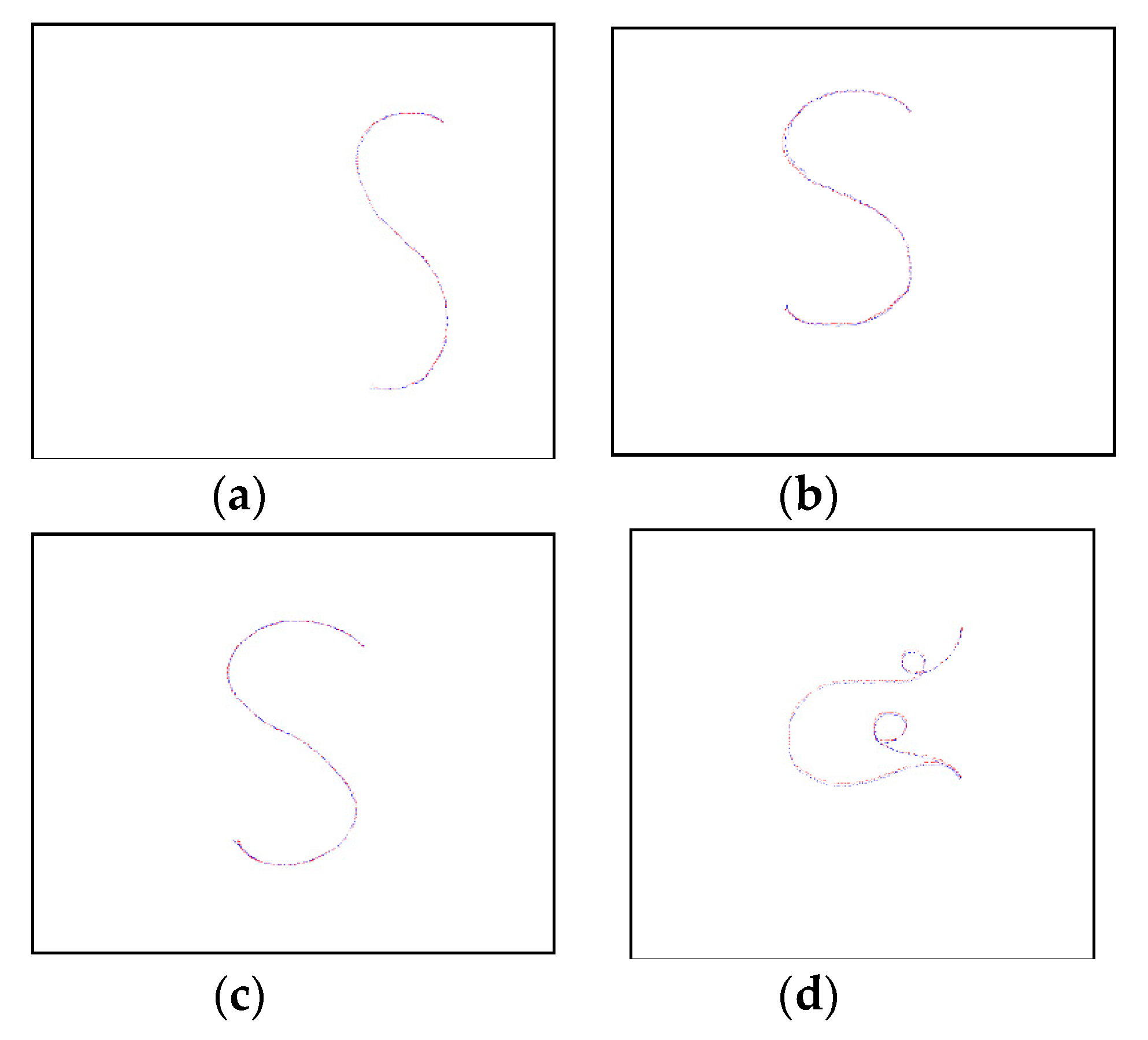
3.1. Performance Evaluation for Curve Transformation

The transformation function in Equation (4) was tested for the performance of the coordinate transformation in translation, rotation, scaling, and complex shape of the edge curves. Ten pairs of synthetic images were used for each of the four scenarios, i.e., 40 pairs in total. Some examples are shown in Figure 6. Here, the reference curves and source curves are shown in red and blue, respectively. Figure 7 shows the example of the curve alignment results between the reference and source curves for all four scenarios. As we anticipated, the transformation function worked really well under naked-eye inspection. For quantitative evaluation, the Hausdroff distance (HD) [25,26] was used to analyze the performance of the method. The HD between set A and set B can be calculated by

$$HD\left(A,B\right)=\max \left(h\left(A,B\right),h\left(B,A\right)\right),$$

(10)

$$h\left(A,B\right)=\underset{a\in A}{\max }\underset{b\in B}{\min }\Vert a-b\Vert ,$$

(11)

$$h\left(B,A\right)=\underset{b\in B}{\max }\underset{a\in A}{\min }\Vert b-a\Vert ,$$

(12)

where $\Vert ·\Vert$ is a distance metric, point sets A = {a₁, a₂, …, a_p} and B = {b₁, b₂, …, b_q}. In this research we choose the Euclidean distance as the distance metric.

The results are shown in

Table 1. The Hausdroff distance for curve alignment between the reference and source curves for all 4 scenarios.

Case	Hausdroff Distance (Pixels)
	Translation	Rotation	Scaling	Complex
1	3.995	3.775	5.885	4.180
2	4.066	3.524	3.837	4.606
3	4.368	4.366	2.864	5.727
4	4.352	5.731	5.638	4.809
5	4.154	4.349	3.248	5.801
6	4.417	6.182	3.315	6.807
7	5.582	6.475	2.988	7.070
8	3.671	7.136	4.338	7.143
9	5.755	7.792	4.177	5.064
10	5.862	6.471	3.981	6.993
Average	4.622	5.580	4.027	5.820
Standard Deviation	0.799	1.482	1.041	1.127

. The average HD values ± standard deviation in pixels between the reference and the transformed images are 4.622 ± 0.799, 5.580 ± 1.482, 4.027 ± 1.041, and 5.820 ± 1.127 pixels, respectively, for translation, rotation, scaling, and complex shape scenarios. The overall result is 5.012 ± 1.317 pixels.

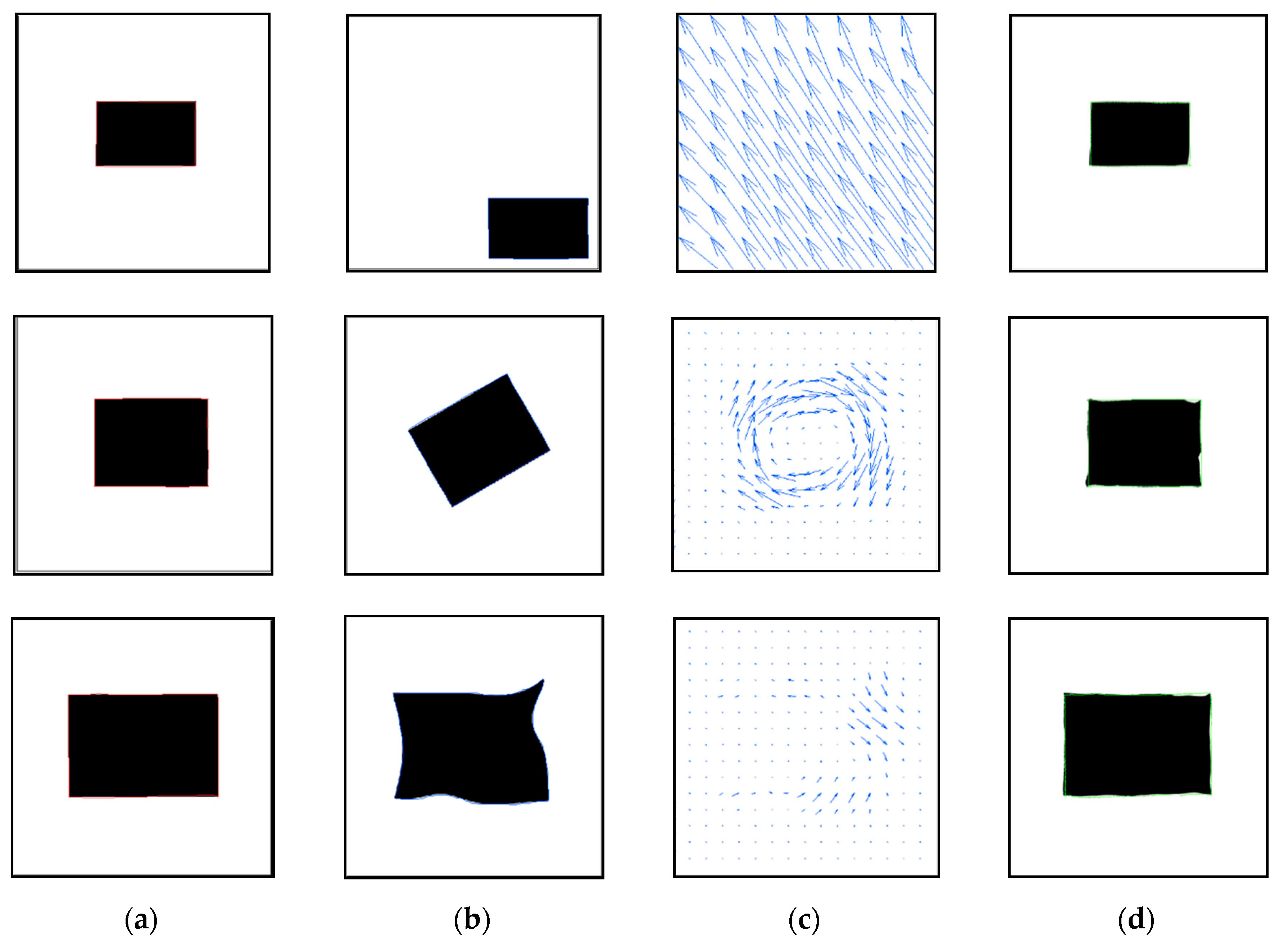
3.2. Performance Evaluation for Binary Image Registration

The synthetic 2D binary images were used to test the performance of the algorithm for the translation, rotation, scaling, deformation, and translated-deformation scenarios, as shown in Figure 8. It should be emphasized once again that the synthetic images were used for the sake of ground truth availability. The parameter α for the weighting Gaussian function was set to 1, and the normalized cross-correlation (NCC) coefficient was used as the evaluation measure for the image registration performance analysis. The examples of results of the binary image registration are shown in Figure 9, whereas the reference curves and source curves are manually delineated in red and blue, respectively. It once again shows that the curve transformation works very well under naked-eye inspection for all binary images under different transformations. The NCC coefficients of 99.39 ± 0.20%, 99.27 ± 0.20%, 99.51 ± 0.20%, 99.51 ± 0.10%, and 99.28 ± 0.20%, were achieved for translation, rotation, scaling, deformation, and translated-deformation, respectively. This demonstrates that the proposed image registration method works really well for binary images.

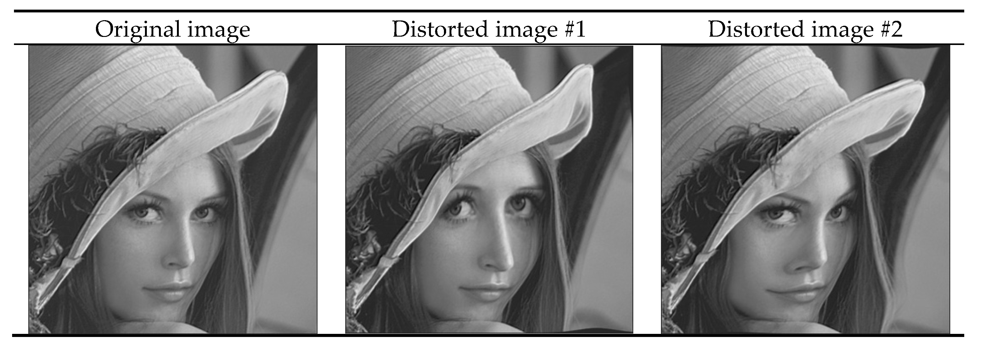
3.3. Performance Evaluation for Grayscale Image Registration

For the grayscale images, a synthetic image (reference image) and some of its transformed versions (source images) are shown in Figure 10. We compared the results of the proposed method with the results from a popular ImageJ plugin named bUnwarpJ [27] and DIRART [28], which is a software suite for deformable image registration and adaptive radiotherapy research, in the image registration and analyzed their performance by using the NCC coefficient. Because of the random nature of how the landmarks are manually chosen in bUnwarpJ, the best two of three results of each image were selected for the sake of fairness. The examples of results from the proposed image registration method are displayed in Figure 11. The comparisons between the proposed method, bUnwarpJ, and DIRART on five transformed images are shown in Figure 12. It can be clearly observed that both bUnwarpJ and the proposed method yield very good results with the NCC coefficients of more than 98% while the proposed method provides higher NCC coefficients than bUnwarpJ in all of the test images. Meanwhile, DIRART clearly yields less NCC coefficients in all of the test images. The average NCC coefficients are 98.71 ± 0.14%, 98.38 ± 0.15%, and 95.20 ± 0.40% for the proposed method, bUnwarpJ, and DIRART, respectively.

We then turned to the classical image of Lena to test our proposed method. We transformed the original image of Lena to 10 different distorted images. Two sample distorted images are shown in Figure 13. Once again, the proposed method, bUnwarpJ, and DIRART were implemented to restore the original image from the distorted ones for the sake of comparison. Figure 14 shows the reference edge curves and source edge curves in red and yellow, respectively. For bUnwarpJ, we manually selected a lot of pairs of landmarks in the reference and source images, as shown in Figure 15, whereas the level set-based method of DIRART uses the intensity for the registration. Figure 16 illustrates the registration results by all three methods. It can be seen visually that the proposed method, bUnwarpJ, and DIRART is able to register the distorted images to the original version. The difference is not easily captured by the naked eye. Hence, some quantitative evaluation measures are needed. In this research, we chose the root–mean–square error (RMSE) and the NCC coefficients between the original (reference) image and distorted/transformed (source) image as the evaluation measures, and the results are shown in

Table 2. Root–mean–square error (RMSE) and NCC coefficients between the original (reference) image and distorted/transformed (source) image for 10 distorted Lena images using the proposed method, bUnwarpJ, and DIRART.

Lena Image no.	No Registration		Proposed Method		bUnwarpJ		DIRART
	RMSE	NCC (%)	RMSE	NCC (%)	RMSE	NCC (%)	RMSE	NCC (%)
1	3252.10	90.41	1607.64	97.65	2220.25	94.20	1631.68	97.57
2	2690.98	93.38	1579.81	97.72	1668.53	96.74	1715.67	97.30
3	3010.36	91.69	1579.81	97.72	1697.29	96.45	2020.65	96.25
4	3249.89	90.27	1738.55	97.23	1828.23	95.98	1926.09	96.58
5	2829.80	92.77	1667.60	97.46	2177.10	94.81	1772.41	97.13
6	2897.92	92.32	1545.06	97.84	2118.51	94.58	1880.80	96.76
7	2392.20	94.81	1344.48	98.35	1814.05	96.30	1355.07	98.32
8	3258.11	90.30	1762.44	97.16	1680.99	96.74	1887.11	96.74
9	2939.54	92.14	1971.31	96.48	2280.70	93.93	2104.41	95.95
10	3185.72	90.64	1982.70	96.41	2227.62	94.39	2218.27	95.47
Average	2970.66	91.87	1677.94	97.40	1971.32	95.41	1851.21	96.81
Standard Deviation	284.13	1.52	195.20	0.60	254.66	1.13	248.16	0.82

. The results show that the proposed method can reduce the RMSE and increase the NCC coefficient compared to the scenario in which no registration is applied. Meanwhile, bUnwarpJ also does the same, but sometimes fails to do so, particularly in areas close to the image border. In contrast, DIRART provides good registration around the image border but fails to do so inside an image. On average, the proposed method can reduce the RMSE from 2970.66 to 1677.94, while bUnwarpJ and DIRART can reduce to 1971.32 and 1851.21, respectively. For the NCC coefficient, on average, the proposed method can increase the value from 91.87% to 97.40%, whereas bUnwarpJ and DIRART can raise it to 95.41% and 96.81%, respectively.

The proposed method focuses on using a set of curve functions as the image transformation. Even though the proposed image registration method works well in many scenarios, it still contains some limitations. The limitations of the proposed method are (1) sequence dependency; the function uses x and y coordination for its information. The corresponding curves were drawn from the reference and the source images and resampled to get the same number of members. The curve fitting fits between the sequence and the value of the coordination; hence, mis-corresponding points lead to misregistration. This limitation does not affect binary images, as shown in the binary image registration experiment, but does affect grayscale images because of its intensity inhomogeneity. In the case of grayscale image registration, multiple edge curves can be used to remedy the limitation, as shown in the grayscale image registration experiment. (2) Segmentation; the proposed method uses the nearest neighborhood method for the image segmentation. This method can cause not only continuity degradation but also rotational limitation. The Gaussian function is used to improve the continuity of moving pixels, but it is well-performed only in the intra-segmented area, not in the inter-segmented area. This limitation can be reduced by using a small number of edge curves or using curves that are far away from one another. The segmentation is computed with respect to the reference edge curves; hence, the members in each group are dependent upon the length of the curves. The number of the moving pixels may be insufficient to be computed for the DVF, especially for higher degrees of rotation.

4. Conclusions

In this research, we propose a new curve-based or edge-based method for image registration that relies on geometric transform. The proposed polynomial fitting and its cubic B-spline conversion method achieve a very good performance in transforming the curves in the reference and source images. Meanwhile, the image registration method is completed by applying the Gaussian function to cope with the discontinuity issue among adjacent segments. The proposed image registration method yields very good results without using the assumptions of affine transformation and non-deformable degradation as used in other methods. This advantage makes the proposed method capable of registering color images without any modification in the algorithm. The registration could also be directly applied when the reference and source images are in different color space, e.g., grayscale and color spaces. Figure 17 demonstrates the good image registration performance by the proposed method when a grayscale image is used as the reference and the color images are used as the source. The first two source (distorted) images are in vintage color, while the other three images are in original color.

For further work, it is possible to improve the proposed method by tackling some existing limitations, such as sequence dependency and area segmentation. These limitations can cause a discontinuity problem and rotational variation that ultimately result in imperfect image registration. Also, from the advantage of the proposed method in that it does not take into account the pixel intensity, image registration between different medical image modalities is highly possible. Because this kind of application to medical diagnosis is very crucial, the medical experts would draw curves for the same organ(s) in different image modalities like MRI, CT, PET, X-Ray, Ultrasound, etc., so that the image registration would be performed, and more useful information from the registration would be available for better diagnosis.

References

1. Ye, Y.; Shan, J.; Bruzzone, L. Robust registration of multimodal remote sensing images based on structural similarity. IEEE Trans. Geosci. Remote Sens. 2017, 55, 2941–2958. [Google Scholar] [CrossRef]
2. Ma, J.; Zhou, H.; Zhao, J. Robust feature matching for remote sensing image registration via locally linear transforming. IEEE Trans. Geosci. Remote Sens. 2015, 53, 6469–6481. [Google Scholar] [CrossRef]
3. Su, Y.; Liu, Z.; Ban, X. Symmetric face normalization. Symmetry 2019, 11, 96. [Google Scholar] [CrossRef]
4. Liu, L.; Jiang, T.; Yang, J. Fingerprint registration by maximization of mutual information. IEEE Trans. Image Process. 2006, 15, 1100–1110. [Google Scholar] [PubMed]
5. Sariyanidi, E.; Gunes, H.; Cavallaro, A. Robust registration of dynamic facial sequences. IEEE Trans. Image Process. 2017, 26, 1708–1722. [Google Scholar] [CrossRef] [PubMed]
6. Li, H.; Manjunath, B.; Mitra, S.H. Registration of 3D multimodality brain images by curve matching. In Proceedings of the 1993 IEEE Conference Record Nuclear Science Symposium and Medical Imaging Conference, San Francisco, CA, USA, 31 October–6 November 1993; pp. 1744–1748. [Google Scholar]
7. Liang, Z.; He, X.; Teng, Q. 3D MRI image super-resolution for brain combining rigid and large diffeomorphic registration. IET Image Process. 2017, 11, 1291–1301. [Google Scholar] [CrossRef]
8. Dong, G.; Yan, H.; Lv, G.; Dong, X. Exploring the utilization of gradient information in SIFT based local image descriptors. Symmetry 2019, 11, 998. [Google Scholar] [CrossRef]
9. Liu, X.; Tao, X.; Ge, N. Fast remote-sensing image registration using priori information and robust feature extraction. Tsinghua Sci. Technol. 2016, 21, 552–560. [Google Scholar]
10. Brock, K.K. Image Processing in Radiation Therapy; Taylor & Francis Group: New York, NY, USA, 2013. [Google Scholar]
11. Li, Y.; Stevenson, R.L. Multimodal image registration with line segments by selective search. IEEE Trans. Cybern. 2017, 47, 1285–1298. [Google Scholar] [CrossRef]
12. Li, J.; Hu, Q.; Ai, M. Robust feature matching for remote sensing image registration based on Lq-estimator. IEEE Geosci. Remote Sens. Lett. 2016, 13, 1989–1993. [Google Scholar] [CrossRef]
13. Razlighi, Q.R.; Kehtarnavaz, N. Spatial mutual information as similarity measure for 3-D brain image registration. IEEE J. Transl. Eng. Health Med. 2014, 2, 27–34. [Google Scholar] [CrossRef] [PubMed]
14. Tagare, H.D.; Rao, M. Why does mutual-information work for image registration? A deterministic explanation. IEEE Trans. Pattern Anal. Mach. Intell. 2015, 37, 1286–1296. [Google Scholar] [CrossRef] [PubMed]
15. Heinrich, M.P.; Jenkinson, M.; Bhushan, M. MIND: Modality independent neighbourhood descriptor for multi-modal deformable registration. Med. Image Anal. 2012, 16, 1423–1435. [Google Scholar] [CrossRef] [PubMed]
16. Reaungamornrat, S.; de Silva, T.; Uneri, A.; Vogt, S.; Kleinszig, G.; Khanna, A.J.; Wolinsky, J.-P.; Prince, J.L.; Siewerdsen, J.H. MIND Demons: Symmetric diffeomorphic deformable registration of MR and CT for image-guided spine surgery. IEEE Trans. Med. Imaging 2016, 35, 2413–2424. [Google Scholar] [CrossRef] [PubMed]
17. Ghassabi, Z.; Shanbehzadeh, J.; Sedaghat, A. An efficient approach for robust multimodal retinal image registration based on UR-SIFT features and PIIFD descriptors. EURASIP J. Image Video Process. 2013, 2013, 25. [Google Scholar] [CrossRef] [Green Version]
18. Cao, W.; Lyu, F.; He, Z. Multi-modal medical image registration based on feature spheres in geometric algebra. IEEE Access 2018, 6, 21164–21172. [Google Scholar] [CrossRef]
19. Xia, M.; Liu, B. Image registration by ‘super-curves’. IEEE Trans. Image Process. 2004, 13, 720–732. [Google Scholar] [CrossRef] [PubMed]
20. Khoualed, S.; Sarbinowski, A.; Samir, C. A new curves-based method for adaptive multimodal registration. In Proceedings of the 5th International Conference on Image Processing, Theory, Tools and Applications, Orleans, France, 10–13 November 2015; pp. 391–396. [Google Scholar]
21. Senneville, B.D.D.; Zachiu, C.; Moonen, C. EVolution: An edge-based variational method for non-rigid multi-modal image registration. Phys. Med. Biol. 2016, 61, 7377–7396. [Google Scholar] [CrossRef]
22. Peng, W.; Tong, R.; Qian, G. A new curves-based local image registration method. In Proceedings of the 1st International Conference on Bioinformatics and Biomedical Engineering, Wuhan, China, 6–8 July 2007; pp. 984–988. [Google Scholar]
23. Rawlings, J.O.; Pantula, S.G.; Dickey, D.A. Polynomial Regression. In Applied Regression Analysis: A Research Tool, 2nd ed.; Casella, G., Fienberg, S., Olkin, I., Eds.; Spinger: New York, NY, USA, 1998; Volume 18, pp. 235–261. [Google Scholar]
24. Unser, M. Splines: A perfect fit for signal processing. Eur. Signal Process. Mag. 1999, 16, 22–38. [Google Scholar] [CrossRef]
25. Chankong, T.; Theera-Umpon, N.; Auephanviriyakul, S. Automatic cervical cell segmentation and classification in Pap smears. Comput. Methods Programs Biomed. 2014, 113, 539–556. [Google Scholar] [CrossRef]
26. Huttenlocher, D.P.; Klanderman, A.; Rucklidge, W.J. Comparing images using the Hausdroff distance. IEEE Trans. Pattern Anal. Mach. Intell. 1993, 15, 850–863. [Google Scholar] [CrossRef]
27. Sorzano, C.O.S.; Thevenaz, P.; Unser, M. Elastic registration of biological images using vector spline regularization. IEEE Trans. Biomed. Eng. 2005, 52, 652–663. [Google Scholar] [CrossRef] [PubMed]
28. Yang, D.; Brame, S.; Naqa, I. Technical Note: DIRART—A software suite for deformable image registration and adaptive radiotherapy research. Med. Phys. 2011, 38, 85–94. [Google Scholar]
Figure 1. Image segmentation by using the nearest neighborhood. (a) Segmentation with respect to the reference curves (curves consisting of red dots), (b) sub-segmentation with respect to the point sequence of the reference curves.
Symmetry 11 01210 g001
Figure 2. Example of the adaptive Gaussian mask with α = 1, µx = 251, µy = 238, σx = 156, and σy = 131.
Symmetry 11 01210 g002
Figure 3. Deformable area along the reference curve (red) with the gradient projected to the source curve (blue).
Symmetry 11 01210 g003
Figure 4. Weighting masks: (a) global weighting mask gW(x, y), (b)–(f) weighting masks of the 5 curves that are combined to form gW(x, y) in (a). The inset in each figure shows the image of the reference curve (red), the source curve (blue), and the corresponding image of the weighting mask.
Symmetry 11 01210 g004
Figure 5. Diagram of the proposed curve-basedimage registration algorithm.
Symmetry 11 01210 g005
Figure 6. The curves for the test of algorithm performance: reference curve (red), source curve (blue), for the transformation (a) translation, (b) rotation, (c) scaling, and (d) complex shape.
Symmetry 11 01210 g006aSymmetry 11 01210 g006b
Figure 7. Performance of curve alignment between the reference curve (red) and source curve (blue) for the curves shown in Figure 3 for the transformation (a) translation, (b) rotation, (c) scaling, and (d) complex shape.
Symmetry 11 01210 g007
Figure 8. Binary image set for performance tests: translation test (ad), rotation test (eh), scaling test (I,k), deformation test (lo) and translated-deformation test (ps). Reference images are shown in (a), (e), (i), (l), and (p).
Symmetry 11 01210 g008aSymmetry 11 01210 g008b
Figure 9. Sample results of the binary image registration from the proposed method (reference edge curve (red) and source edge curve (blue)): (a) reference images, (b) source images, (c) deformation vector fields (DVFs), and (d) registered images, for the cases of translation (top), rotation (middle), and deformation (bottom).
Symmetry 11 01210 g009
Figure 10. Grayscale image set of the performance test: (a) reference image and (bd) source images.
Symmetry 11 01210 g010
Figure 11. Sample results of the grayscale image registration from the proposed method (reference edge curve (red) and source edge curve (blue)): (a) reference images, (b) source images, (c) DVFs, and (d) registered images.
Symmetry 11 01210 g011
Figure 12. The comparison of NCC coefficients between the proposed image registration method, bUnwarpJ, and DIRART in the grayscale image registration.
Symmetry 11 01210 g012
Figure 13. Original Lena image and 2 examples of its distorted versions.
Symmetry 11 01210 g013
Figure 14. Reference edge curves (red) and source edge curves (yellow) in the proposed method.
Symmetry 11 01210 g014
Figure 15. Landmark pairs in reference and source images in bUnwarpJ.
Symmetry 11 01210 g015
Figure 16. Sample image registration results from the proposed method, bUnwarpJ, and DIRART.
Symmetry 11 01210 g016
Figure 17. Sample image registration results from the proposed method when the reference image is in grayscale and the source images are in color.
Symmetry 11 01210 g017aSymmetry 11 01210 g017b