Abstract
We consider the model of Dirac fermions coupled to gravity as proposed, in which superluminal velocities of particles are admitted. In this model an extra term is added to the conventional Hamiltonian that originates from Planck physics. Due to this term, a closed Fermi surface is formed in equilibrium inside the black hole. In this paper we propose the covariant formulation of this model and analyse its classical limit. We consider the dynamics of gravitational collapse. It appears that the Einstein equations admit a solution identical to that of ordinary general relativity. Next, we consider the motion of particles in the presence of a black hole. Numerical solutions of the equations of motion are found which demonstrate that the particles are able to escape from the black hole.
1. Introduction
The Schwarzschild black hole (BH) solution [1,2] may be brought to a form, which is especially useful for the consideration of the motion of matter. This is the so-called Painlevé-Gullstrand (PG) black hole [3,4]. In the corresponding reference frame space–time looks like flat space falling down to the center of the BH with velocity that depends on the distance to the center. Such a representation also exists for the Reissner-Nordstrom BH and even for the Kerr BH [5,6]. The structure of the BH solution in the PG reference frame prompts to consider the analogy to the motion of a fluid in the laboratory. Such an analogy has been considered in the framework of the theory of 3He superfluid in [7]. It allows to calculate in a demonstrative way Hawking radiation [8] (see also, for example, [9,10,11,12] and references therein).
The consideration of Dirac fermions in the PG reference frame leads to the unexpected observation that inside the BH the fermion states with vanishing energy form the surface in momentum space. In equilibrium, at vanishing temperature, it becomes the Fermi surface and separates the region of occupied quantum states from the region of the vacant ones. For the ordinary Dirac fermions such a surface is open and infinite. The analogy with condensed matter physics suggests that the particle Hamiltonian is to be modified in such a way so that the resulting Fermi surface will become finite and closed. It has been proposed in [13] that such a modification occurs due to Planck physics. The corresponding term has been added to the Dirac Hamiltonian. It leads to several consequences for BH physics. First of all, the analogy to the BH in the PG reference frame has been found within the class of the recently discovered materials called Weyl semimetals [14,15,16,17,18,19,20,21]. Bloch electrons within those materials behave similarly to the elementary particles. In the special type of such materials called the type II Weyl semimetals (WSII) [22,23,24] the dependence of energy of electrons on momenta [25] possesses an analogy to that of the particles in the interior of the BH [26,27].
In [28,29,30] it was noticed that if a closed finite Fermi surface inside the BH is formed, there should exist particles that escape from the BH without tunneling. In the present paper we take a step back and consider the model proposed in [13] on the classical level. We suppose that a careful consideration of the classical dynamics should precede the more sophisticated discussion of the quantum BH, although the extra term added to the particle Hamiltonian becomes relevant at Planck energies.
This extra term contains the time—like four—vector . In the Painlevé-Gullstrand reference frame it marks the direction of time. In the covariant theory there should be no such preferred direction of time. We assume that it appears as a result of a dynamical symmetry breaking. This symmetry breaking, in turn, results in the appearance of the massless Goldstone modes. Here we shall not discuss the physics of those massless excitations.
First of all, we propose the covariant formulation of the discussed model. It contains the vector field , which, after the spontaneous breakdown, acquires its particular value that points in the direction of time in the Painlevé-Gullstrand reference frame. The classical equations of motion for the corresponding point—like particles admit motion with superluminal velocity. Therefore, unsurprisingly, the particles may escape from the black hole already at the classical level. For the discussion of the theories that admit superluminal velocity of particles we refer to [31,32].
The paper is organized as follows. First of all, in Section 2 we recall the general properties of the Dirac fermions in the PG reference frame in the presence of the charged BH. In Section 3 we propose the covariant formulation of the model of [13] and derive its classical limit. In Section 4 we derive the expression for the stress–energy tensor of the noninteracting particles in the PG reference frame. In Section 5 the gravitational collapse in this model is considered. In Section 6 we present the results of the numerical solution of the classical equations of motion for the motion of particles in the presence of the existing black hole (at the stage when the gravitation collapse is finished). The physical significance of the results is dicussed in the concluding Section 7. Throughout the paper we use the units with .
2. Dirac Fermions in the Black Hole in the Painleve–Gullstrand Reference Frame
In the present paper we will be interested in neutral black holes. However, we start our consideration from the ansatz that corresponds to a charged black hole [5,6] (see also [33,34]). The charge is assumed to be small, so that it modifies the BH solution in the small vicinity of the BH center. We will add also another modification in the small vicinity of the center, which will cause the metric to be regular everywhere. Thus we start from the charged black hole metric in the PG coordinates
Here the expression
may be considered as a velocity of space falling towards the center of the BH. Q is the charge of the BH, is the Plank mass, while M is the BH mass.
The vielbein is given by
and the inverse vielbein is
The metric is equal to
where .
The action for the Weyl fermions has the form
where symbols R (L) mark the right-handed/left-handed fermions. Here are the Pauli matrices. Their Hamiltonians are
The Dirac mass term mixes the right-handed and the left-handed fermions
It appears that the spin connection does not enter this action. Next, following [13], we introduce the term that breaks the Lorentz invariance:
Here parameter is assumed to be of the order of the Plank mass. For the velocity v becomes imaginary. It is pausible that due to the interaction with matter the dependence of v on r is modified within the BH, and v remains real and tends to zero at (see also [5]). In the present paper we model this form of v via the following modification
with
The resulting form of is represented in Figure 1 in the system of units with at and . This modification changes the form of the gravitational field only close to the center of the black hole. It is expected that in the small vicinity of the center of the black hole the Einstein equations are to be modified because otherwise the value of v becomes imaginary, which is unphysical. Equation (9) is not derived from any particular equations of motion and, therefore, represents a modification of the metric that follows from the requirement that v remains real.
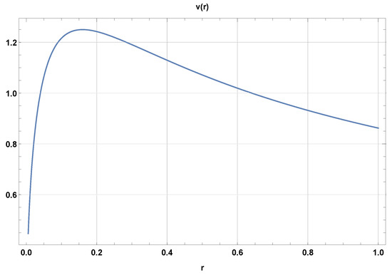
Figure 1.
Velocity of “vacuum” (vertical axis) as a function of r (horizontal axis) for and .
The two horizons are placed at
and
For ordinary Dirac fermions with mass m of Equation (7). The horizons given by Equations (10) and (11) are defined as the surfaces, where the vacuum velocity becomes equal to the speed of light. At the Fermi point appears. Between the two horizons at there is the type II Dirac point, while is larger than the speed of light. Notice that this, in itself, yet does not mean that the velocity of real particles does exceeds the speed of light [35]. In fact, a particle with a conventional action that does not break Lorentz invariance still moves with a velocity smaller than the speed of light. A “Vacuum velocity” exceeding the speed of light then guarantees that such a particle cannot escape from the BH interior. However, as we will see below, the Lorentz breaking term in the action of Equation (8) leads to the superluminal motion of the particle excitation, and to its ability to escape from the BH.
Neglecting the derivatives of we come to the following expression for the particle energy
Thus, assuming that varies slowly, we come to the conclusion that between the two horizons the particle energy vanishes along the closed surface in momentum space. Its form is represented in Figure 2 for a particular choice of the parameters. It is worth mentioning that the Hamiltonian of the form of Equation (12) admits motion with the superluminal velocity on the classical level. Therefore, unsurprisingly, in the considered model the particles are able to escape from the black hole.
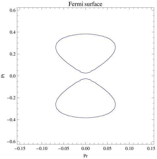
Figure 2.
The typical Fermi surface form in the plane within the black hole at the values of parameters , , and . Here the vertical axis corresponds to while the horizontal axis corresponds to . For these values the external horizon is placed at . We represent the Fermi surface at .
Notice again that the only meaning of parameters Q and in Equation (9) is the modification of the neutral black hole solution in the small vicinity of . This modification regularizes the theory close to the center of the black hole. Far from the gravitational field corresponds to the one of the neutral black hole.
3. Covariant Formulation of the Theory and Its Classical Limit
Here we propose the covariant modification of the model of [13] considered in the previous section. Namely, we consider the Dirac field with action
Here we denote and The spin connection is given by
Here ; . For the details see References [36,37,38,39]. By n we denote the vector field. Its action may be taken in the form
At sufficiently large values of this vector field becomes non-propagating. Its vacuum average gives rise to the spontaneous breakdown of Lorentz symmetry. Neglecting spin degrees of freedom we will finally come to the dispersion of the form of Equation (12). The 4-vector n in the PainleveGullstrand reference frame is constant and marks the time direction:
Correspondingly, . The appearance of this vector breaks the group of general coordinate transformations in four-dimensional space–time to the group of general coordinate transformations in three-dimensional space. As a result three massless Goldstone modes would appear corresponding to the broken boosts if there are no gauge bosons. However, if a dynamical gravity with an independent spin connection field is considered (this means that we consider the fluctuations of both metric and spin connection around the classical solution of the Palatini equation; this equation is also known as the Einstein equation written in the first order formalism), then the mentioned Goldstone bosons are eaten by the dynamical field of the spin connection thus giving rise to an effective mass term for the latter. The same mechanism may also have its incarnation in Riemannian gravity, in which the spin connection is expressed uniquely through the metric. This, however, remains out of the scope of the present paper. Notice that in massive gravity a certain modification of the BH evaporation process has been predicted [40,41,42] (see also [43]).
The only component of the spin connection (in spherical coordinates) is . This term disappears from the first term in the Painlevé-Gullstrand reference frame. However, it is essential for the calculation of the stress–energy tensor.
The first step towards the classical theory is the consideration of the above model with the spin neglected. This corresponds to the consideration of the scalar field instead of the Dirac spinor and the corresponding action. Hence the theory is that of a scalar field with the action
There is no precise correspondence between Equations (13) and (15). In the transition the spin degrees of freedom and the corresponding terms in the lagrangian were neglected. The variation of this action with respect to gives the wave equation
In the semiclassical limit we substitute by momentum and by energy . This gives the following relation for
In the Painlevé-Gullstrand reference frame we get
This equation gives rise to the classical particle Hamiltonian of [13] given by Equation (12).
4. The Stress–Energy Tensor of the Non-Interacting Classical Particles
4.1. General Expression for the Stress–Energy Tensor
In this section we consider matter that consists of the non-interacting particles. Our aim is to consider the gravitational collapse. Therefore, following [44] we consider the generalization of the Painlevé-Gullstrand spacetime:
with
Function enters Equation (19) that defines the vacuum velocity. The latter, in turn enters Equation (18) for the metric. If we substitute the ansatz for metric of Equation (18) to the Einstein equations, we obtain equation for the function . It is to be obtained through the solution of Einstein equations.
While we are going to calculate the stress–energy tensor of the classical system, we prefer to start from the model of the scalar field with action Equation (15). We will calculate the stress–energy tensor of the corresponding quantum system and take the classical limit at the end of the calculation. We are to calculate the stress–energy tensor through the variation of action with respect to the variation of metric
Notice that . In a similar way we calculate the current density as
In the semiclassical limit the oscillating factors in the radial wave functions are given by while the electric current may be identified with the product of the particle density and the velocity of substance. This leads to the following semiclassical relation in the generalized Painlevé-Gullstrand reference frame
Here is the particle density. The number of particles in a small volume around the given space–time point is equal to . It is supposed that all these particles have equal values of energy , velocity , and momentum . Those quantities are related to each other via the classical equations of motion
The above equations enable us to relate the absolute value of with the physical quantities and . In an arbitrary reference frame we have the similar relation
Here
is the density of particles. Therefore, in the Painlevé-Gullstrand coordinates we identify
while in the arbitrary reference frame
In the same limit the stress–energy tensor is given by
The equations of motion give
4.2. The Stress–Energy Tensor in the Limit
Let us demonstrate how Equation (23) gives rise to the conventional stress–energy tensor of the non-interacting particles in the limit . We have
In the generalized PG reference frame we have
This gives
Here is the four-velocity of the particles/substance. We come to the conventional expression
where is the energy density in the rest frame of the medium (notice that is the particle density in the given reference frame while is the particle density in the rest frame).
4.3. Expression for the Stress–Energy Tensor for Finite in the Case When the Substance Is Co-Moving with the Space Flow
In the general case the following expression for the stress–energy tensor should be obtained
The scalar functions depend on the four-velocity u, the four-vector n, the constant , and the energy density . In the important particular case, when velocity of substance everywhere is equal to , the classical equations of motion give and we obtain the especially simple result
5. Description of the Gravitational Collapse in the Generalized Painlevé-Gullstrand Coordinates
In this section we consider the gravitational collapse of matter that consists of the non-interacting neutral particles (for the discussion of the collapse of the charged matter see, e.g., [45]). Those particles being placed into the Painlevé-Gullstrand spacetime have the Hamiltonian
The generalization of the PG spacetime [44] has the following metric
with
The function is to be obtained through the solution of Einstein equation.
It was shown above that the noninteracting matter with the Hamiltonian of [13] has stress–energy tensor equal to that of the conventional matter in the generalized Painlevé-Gullstrand coordinates in the important particular case, when at each point the velocity of matter is precisely equal to . The problem for the gravitational collapse of matter with this stress–energy tensor is solved in [44].
For the noninteracting particles (perfect fluid) in the above particular case the energy–momentum tensor has the form
Here is the energy density, and the radial four-velocity of the fluid. Correspondingly . For the definiteness let us assume that is directed along the x axis. Then
It follows from the derivation of [44] that
and
We come to the following pattern of the gravitational collapse. If the velocity of matter at the starting moment is equal to the function of the generalized Painlevé-Gullstrand reference frame, and everywhere the three-momentum of the particles vanishes at , then the Einstein equations have the solution given by Equations (32) and (33). Thus, matter contracts towards the center of the BH together with the “falling” space. This gives
As a result, the position of the horizon (where the velocity equals 1) depends on time
One can see that at each finite value of t the velocity of space fall vanishes for only. The space–time metric remains regular everywhere.
The collapse of dust placed within a sphere leads at to the formation of the ordinary PainlevéGullstrand BH (see [44]). In the next section we will consider the classical motion of particles in the formed BH regularized in the small vicinity of its center as explained in Section 2.
6. Classical Dynamics of Particles
In this section we discuss the dynamics of the single particle moving in the radial direction in the presence of the existing black hole. In the Gullstrand-Painleve coordinates metric does not depend on time. The classical Hamiltonian of the particle in the presence of the black hole has the form
For the radial motion the corresponding classical equations are
The Fermi surface for the particular value of r crosses the axis of radial momentum at
One can see that the Fermi surface is not formed immediately behind the external horizon. Instead, it is formed at
The typical classical trajectories of the particles are calculated and represented in Figure 3, Figure 4 and Figure 5. The particles that fall together with the “vacuum” reach the center of the black hole and stay there. However, if the initial momentum is nonzero, the particles that have fallen down to the black hole receive large values of radial momentum in a small vicinity of the BH center. As a result, they escape from the BH. If the initial momentum was directed to the center of the BH, then the particle traverses the BH and escapes it from a diametrically opposite point. If the initial momentum is in the opposite direction, then its velocity reverses the sign close to the center of the BH, the particle is turned back. In the exterior of the black hole the momentum is decreased, and the particle velocity changes the sign again. The particle falls down again thus forming oscillations.
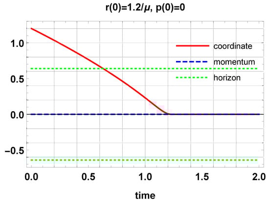
Figure 3.
The radial trajectory of the particle that falls down to the black hole (red solid line): The dependence of radial coordinate r in the units of on time (in the same units); radial momentum in the units of as a function of time (dashed blue line). The vertical axis corresponds to r and , while the horizontal axis corresponds to time. Values of parameters: , and , while . The external horizon is represented by the dotted green line. The particle starts falling at and . One can see that this particle falls together with “vacuum”. It reaches the center of the BH and stays there.
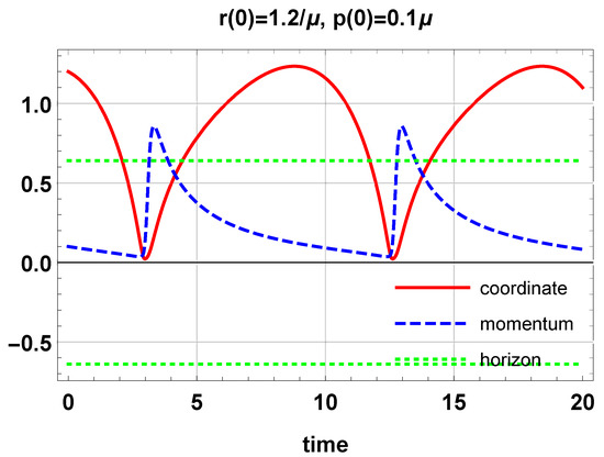
Figure 4.
The radial trajectory of the particle that falls down to the black hole and escapes from it (red solid line): The dependence of radial coordinate r in the units of on time (in the same units); radial momentum in the units of as a function of time (dashed blue line). The vertical axis corresponds to r and , while the horizontal axis corresponds to time. Values of parameters: , , and . The external horizon is represented by the dotted green line. The particle starts falling at and . This particle falls more slow than “vacuum”. It reaches the vicinity of the center of the BH. There the repulsion force pushes it away, it escapes from the BH, then falls again, etc.
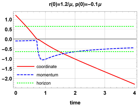
Figure 5.
The radial trajectory of the particle that traverses the black hole (red solid line): The dependence of radial coordinate r in the units of on time (in the same units); radial momentum in the units of as a function of time (dashed blue line). The vertical axis corresponds to r and , while the horizontal axis corresponds to time. Values of parameters: , , and . The external horizon is represented by the dotted green line. The particle starts falling at and . This particle falls faster than “vacuum”. It reaches the center of the BH and crosses it. The repulsion force accelerates it, and the particle escapes at the diametrically opposite point.
Our numerical data allow to estimate the typical time period of those oscillation for (when the amplitude is of the order of the horizon)
(see Figure 6). The region of parameters that leads to Equation (36) corresponds to the situation typical for the large black holes with masses much larger than the plank mass. The value of the oscillation period for the elementary particle in the presence of the solar mass BH (in seconds) is
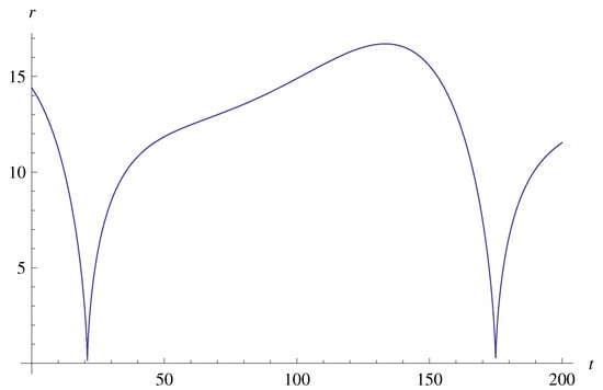
Figure 6.
The radial trajectory of the particle that falls down to the black hole and escapes from it: The dependence of radial coordinate r in the units of on time. The vertical axis corresponds to r, while the horizontal axis corresponds to time. Values of parameters: , , and . The external horizon h is not represented here, but the motion starts at and . It is supposed that this figure represents qualitatively the typical trajectory for .
7. Conclusions
To conclude, in the present paper we consider the model of noninteracting Dirac fermions with the modified Hamiltonian proposed in [13]. In this model the extra ∼ term is added to the Dirac Hamiltonian. First of all, we propose the covariant generalization of this model. The resulting field theory is defined in terms of the Dirac spinor field. It depends on the background field that equals in the Painlevé-Gullstrand reference frame. The field n points into the direction of time in this coordinate system. It appears as a result of the spontaneous symmetry breaking.
Next, we consider the classical limit of the obtained system. First, neglecting the spin we come to the theory of the scalar field with a certain action (depending on n). Next, we consider the semiclassical approximation within this theory, which gives both the classical particle Hamiltonian of [13], and the implicitly defined expression for the stress–energy tensor of medium that consists of the noninteracting particles. It appears that the Einstein equations admit the gravitational collapse solution identical to that of the system of the conventional noninteracting particles. This solution describes the dust falling together with space–time.
Finally, we describe the dynamics of particles in the presence of the existing black holes. It appears that only those particles remain inside the BH, which fall with velocity v entering the expression for the Painlevé Gullstrand metric. The particles that fall towards the center of the BH with nonzero momentum either pass through the BH and reach infinity or turn back at the small vicinity of the BH center, escape from the BH, and proceed the oscillatory motion. Therefore, this means that the particles are able to move with the velocity larger than the speed of light. While the considered theory is manifestly covariant (as explained in Section 3), the geodesic lines are already not the solutions of the classical equations of motion of point-like particles. The solutions of those equations may correspond to the space-like pieces of the particle worldlines, which does not contradict the general covariance.
According to our estimates for the BH with the solar mass the typical period of the mentioned oscillations (when interactions are neglected) is smaller than one second. This means that if the effective Hamiltonian of particles indeed receives the considered contribution from Planck physics, then we cannot ignore it in the dynamics: Matter that has fallen to the BH escapes from it within the observable period of time.
We started our consideration from the model of Dirac fermions. However, then the system is considered classically. This means, that both spin and nontrivial statistics are neglected. In that sense our results are valid both for the fermionic particles and for the bosonic particles in the presence of black holes, and also for both bosonic and fermionic matter participating in the gravitational collapse.
It is worth mentioning that close to the center of the BH quantum effects may become important. The classical analysis presented here describes completely the motion of particles if the modification of the metric of Equation (9) occurs at distances much larger than the inverse Plank mass. Otherwise quantum effects will become relevant. However, even then the classical analysis remains important and represents a first step towards the development of a quantum description.
Author Contributions
The authors contributed equally to this work.
Funding
This research received no external funding.
Acknowledgments
One of the authors (M.A.Z.) kindly acknowledges useful discussions with G.E. Volovik.
Conflicts of Interest
The authors declare no conflict of interest.
References
- Schwarzschild, K. Uber das Gravitationsfeld eines Massenpunktes nach der Einsteinschen Theorie; Sitzungsberichte der Koniglich Preussischen Akademie der Wissenschaften: Berlin, Germany, 1916; pp. 189–196. [Google Scholar]
- Schwarzschild, K. Uber das Gravitationsfeld einer Kugel aus inkompressibler Flussigkeit nach der Einsteinschen Theorie; Sitzungsberichte der Koniglich Preussischen Akademie der Wissenschaften: Berlin, Germany, 1916; pp. 424–434. [Google Scholar]
- Gullstrand, A. Allgemeine Losung des statischen Einkorperproblems in der Einsteinschen Gravitationstheorie. Arkiv. Mat. Astron. Fys. 1922, 16, 1–15. [Google Scholar]
- Painleve, P. La mecanique classique et la theorie de la relativite. C. R. Acad. Sci. (Paris) 1921, 173, 677–680. [Google Scholar]
- Hamilton, A.J.S.; Lisle, J.P. The River model of black holes. Am. J. Phys. 2008, 76, 519. [Google Scholar] [CrossRef]
- Doran, C. A New form of the Kerr solution. Phys. Rev. D 2000, 61, 067503. [Google Scholar] [CrossRef]
- Volovik, G.E. Simulation of Painleve-Gullstrand black hole in thin He-3—A film. JETP Lett. 1999, 69, 705. [Google Scholar] [CrossRef]
- Hawking, S.W. Particle Creation by Black Holes. Commun. Math. Phys. 1975, 43, 199. [Google Scholar] [CrossRef]
- Parikh, M.K.; Wilczek, F. Hawking radiation as tunneling. Phys. Rev. Lett. 2000, 85, 5042. [Google Scholar] [CrossRef]
- Akhmedov, E.T.; Akhmedova, V.; Singleton, D. Hawking temperature in the tunneling picture. Phys. Lett. B 2006, 642, 124. [Google Scholar] [CrossRef]
- Jannes, G. Hawking radiation of E < m massive particles in the tunneling formalism. JETP Lett. 2011, 94, 18. [Google Scholar] [CrossRef]
- Volovik, G.E. The Universe in a Helium Droplet; Clarendon Press: Oxford, UK, 2003. [Google Scholar]
- Huhtala, P.; Volovik, G.E. Fermionic microstates within Painleve-Gullstrand black hole. J. Exp. Theor. Phys. 2002, 94, 853–861. [Google Scholar] [CrossRef]
- Parameswaran, S.; Grover, T.; Abanin, D.; Pesin, D.; Vishwanath, A. Probing the chiral anomaly with nonlocal transport in Weyl semimetals. Phys. Rev. X 2014, 4, 031035. [Google Scholar]
- Vazifeh, M.; Franz, M. Electromagnetic response of weyl semimetals. Phys. Rev. Lett. 2003, 111, 027201. [Google Scholar] [CrossRef] [PubMed]
- Chen, Y.; Wu, S.; Burkov, A. Axion response in Weyl semimetals. Phys. Rev. B 2013, 88, 125105. [Google Scholar] [CrossRef]
- Chen, Y.; Bergman, D.; Burkov, A. Weyl fermions and the anomalous Hall effect in metallic ferromagnets. Phys. Rev. B 2013, 88, 125110. [Google Scholar] [CrossRef]
- Ramamurthy, S.T.; Hughes, T.L. Patterns of electro-magnetic response in topological semi-metals. arXiv 2014, arXiv:1405.7377. [Google Scholar]
- Zyuzin, A.A.; Burkov, A.A. Topological response in Weyl semimetals and the chiral anomaly. Phys. Rev. B 2012, 86, 115133. [Google Scholar] [CrossRef]
- Goswami, P.; Tewari, S. Axionic field theory of (3+1)-dimensional Weyl semi-metals. Phys. Rev. B 2013, 88, 245107. [Google Scholar] [CrossRef]
- Liu, C.-X.; Ye, P.; Qi, X.-L. Chiral gauge field and axial anomaly in a Weyl semimetal. Phys. Rev. B 2013, 87, 235306. [Google Scholar] [CrossRef]
- Soluyanov, A.A.; Gresch, D.; Wang, Z.; Wu, Q.; Troyer, M.; Dai, X.; Bernevig, B.A. Type-II Weyl Semimetals. Nature 2015, 527, 495–498. [Google Scholar] [CrossRef]
- Schonemann, R.; Aryal, N.; Zhou, Q.; Chiu, Y.-C.; Chen, K.-W.; Martin, T.J.; McCandless, G.T.; Chan, J.Y.; Manousakis, E.; Balicas, L. Fermi surface of the Weyl type-II metallic candidate WP2. Phys. Rev. B 2017, 96, 121108. [Google Scholar] [CrossRef]
- Rhodes, D.; Schonemann, R.; Aryal, N.; Zhou, Q.; Zhang, Q.R.; Kampert, E.; Chiu, Y.-C.; Lai, Y.; Shimura, Y.; McCandless, G.T.; et al. Bulk Fermi-surface of the Weyl type-II semi-metallic candidate MoTe2. Phys. Rev. B 2017, 96, 165134. [Google Scholar] [CrossRef]
- Volovik, G.E.; Zubkov, M.A. Emergent Weyl spinors in multi-fermion systems. Nucl. Phys. B 2014, 881, 514. [Google Scholar] [CrossRef]
- Volovik, G.E. Black hole and Hawking radiation by type-II Weyl fermions. JETP Lett. 2016, 104, 645. [Google Scholar] [CrossRef]
- Nissinen, J.; Volovik, G.E. Type-III and IV interacting Weyl points. JETP Lett. 2017, 105, 447–452. [Google Scholar] [CrossRef]
- Zubkov, M.A. The black hole interior and the type II Weyl fermions. Mod. Phys. Lett. A 2018, 33, 1850047. [Google Scholar] [CrossRef]
- Zubkov, M.A. Analogies between the Black Hole Interior and the Type II Weyl Semimetals. Universe 2018, 4, 135. [Google Scholar] [CrossRef]
- Zubkov, M.A.; Lewkowicz, M. The type II Weyl semimetals at low temperatures: Chiral anomaly, elastic deformations, zero sound. Ann. Phys. 2018, 399, 26–52. [Google Scholar] [CrossRef]
- Babichev, E.; Mukhanov, V.; Vikman, A. k-Essence, superluminal propagation, causality and emergent geometry. JHEP 2008, 0802, 101. [Google Scholar] [CrossRef]
- Dubovsky, S.; Gregoire, T.; Nicolis, A.; Rattazzi, R. Null energy condition and superluminal propagation. JHEP 2006, 2006, 025. [Google Scholar] [CrossRef]
- Dale, R.; Saez, D. Spherical symmetric dust collapse in vector-tensor gravity. Phys.Rev. D 2018, 98, 064007. [Google Scholar] [CrossRef]
- Moffat, J.W. Black holes in Modified Gravity (MOG). Eur. Phys. J. C 2015, 75, 175. [Google Scholar] [CrossRef]
- Arraut, I.; Batic, D.; Nowakowski, M. Velocity and velocity bounds in static spherically symmetric metrics. Central Eur. J. Phys. 2011, 9, 926. [Google Scholar] [CrossRef]
- Alexandrov, S. Immirzi parameter and fermions with non-minimal coupling. Class. Quant. Grav. 2008, 25, 145012. [Google Scholar] [CrossRef]
- Vladimirov, A.A.; Diakonov, D. Phase transitions in spinor quantum gravity on a lattice. Phys. Rev. D 2012, 86, 104019. [Google Scholar] [CrossRef]
- Diakonov, D. Towards lattice-regularized Quantum Gravity. arXiv 2011, arXiv:1109.0091. [Google Scholar]
- Diakonov, D.; Tumanov, A.G.; Vladimirov, A.A. Low-energy general relativity with torsion: A systematic derivative expansion. Phys. Rev. D 2011, 84, 124042. [Google Scholar] [CrossRef]
- Arraut, I. The black hole radiation in massive gravity. Universe 2018, 4, 27. [Google Scholar] [CrossRef]
- Arraut, I. On the apparent loss of predictability inside the de-Rham-Gabadadze-Tolley non-linear formulation of massive gravity: The Hawking radiation effect. EPL 2015, 109, 10002. [Google Scholar] [CrossRef]
- Arraut, I. Path-integral derivation of black-hole radiance inside the de-Rham-Gabadadze-Tolley formulation of massive gravity. Eur. Phys. J. C 2017, 77, 501. [Google Scholar] [CrossRef]
- Arraut, I. Black-hole evaporation from the perspective of neural networks. EPL 2018, 124, 50002. [Google Scholar] [CrossRef]
- Kanai, Y.; Siino, M.; Hosoya, A. Gravitational collapse in Painleve-Gullstrand coordinates. Prog. Theor. Phys. 2011, 125, 1053. [Google Scholar] [CrossRef]
- Krasinski, A.; Bolejko, K. Avoidance of singularities in spherically symmetric charged dust. Phys. Rev. D 2006, 73, 124033. [Google Scholar] [CrossRef]


© 2019 by the authors. Licensee MDPI, Basel, Switzerland. This article is an open access article distributed under the terms and conditions of the Creative Commons Attribution (CC BY) license (http://creativecommons.org/licenses/by/4.0/).