Article

Implementation of Artificial Intelligence for Classification of Frogs in Bioacoustics

1
Department of Mechanical Engineering, National Cheng Kung University, Tainan 701, Taiwan
2
Smart Machinery and Intelligent Manufacturing Research Center, National Formosa University, Yunlin 632, Taiwan
3
Department of Information Management, National Formosa University, Yunlin 632, Taiwan
4
Fudan Senior High School, Taoyuan 324, Taiwan
*
Author to whom correspondence should be addressed.
Symmetry 2019, 11(12), 1454; https://doi.org/10.3390/sym11121454
Submission received: 9 November 2019 / Revised: 22 November 2019 / Accepted: 24 November 2019 / Published: 26 November 2019

Abstract

:
This research presents the implementation of artificial intelligence (AI) for classification of frogs in symmetry of the bioacoustics spectral by using the feedforward neural network approach (FNNA) and support vector machine (SVM). Recently, the symmetry concept has been applied in physics, and in mathematics to help make mathematical models tractable to achieve the best learning performance. Owing to the symmetry of the bioacoustics spectral, feature extraction can be achieved by integrating the techniques of Mel-scale frequency cepstral coefficient (MFCC) and mentioned machine learning algorithms, such as SVM, neural network, and so on. At the beginning, the raw data information for our experiment is taken from a website which collects many kinds of frog sounds. This in fact saves us collecting the raw data by using a digital signal processing technique. The generally proposed system detects bioacoustic features by using the microphone sensor to record the sounds of different frogs. The data acquisition system uses an embedded controller and a dynamic signal module for making high-accuracy measurements. With regard to bioacoustic features, they are filtered through the MFCC algorithm. As the filtering process is finished, all values from ceptrum signals are collected to form the datasets. For classification and identification of frogs, we adopt the multi-layer FNNA algorithm in machine learning and the results are compared with those obtained by the SVM method at the same time. Additionally, two optimizer functions in neural network include: scaled conjugate gradient (SCG) and gradient descent adaptive learning rate (GDA). Both optimization methods are used to evaluate the classification results from the feature datasets in model training. Also, calculation results from the general central processing unit (CPU) and Nvidia graphics processing unit (GPU) processors are evaluated and discussed. The effectiveness of the experimental system on the filtered feature datasets is classified by using the FNNA and the SVM scheme. The expected experimental results of the identification with respect to different symmetry bioacoustic features of fifteen frogs are obtained and finally distinguished.

1. Introduction

The lives on Earth are closely relevant to environmental changes on various spatial and temporal scales [1]. The success of human societies intimately relies on the living elements of natural and managed systems. Even though geographical range limits of species are naturally changing with time-variants, climate change is gradually impelling a universal redistribution of lives on Earth [2,3]. To know more about the life distribution or migration of animals, related prospective detection and research in bioacoustics should be conducted [4,5].
There are obvious characteristics of animals that can be used as sensors for the early detection of what are most concerned. Behavior [6,7] and sound [8,9,10] are both such characteristics. It is probable to make use of sound to detect some phenomena, no matter which acoustic field it is [11]. If things produce sounds, there are existing ways to interpret and predict possible meanings conveyed by sound. For example, things that are in good condition sound energetic, whereas they sound obviously weak under bad conditions. As a specific example, emission with a choking sound as well as abnormal acoustic/vibration energy of automobiles might indicate some problems [12]. By the same token, different sound features may symbolize corresponding characteristics of an entity. This also explains why sounds are commonly used by animals to communicate or interact [8,13]. From practical experience, distinct animal acoustic features reveal different contents of meaningful information [14]. Furthermore, the same information conveyed by a particular sound can be transformed into other appearances without loss of its meaning. For example, even when they are under water, sounds generated by some animals are converted to a series of bubbles [15,16]. Owing to the mass acoustic communication among animals, automated acoustic monitoring can not only give an appropriate way to survey different species in their natural way of life, but can also provide a convenient and cost-effective way to monitor target species efficiently. At the same time, it can reduce the need of manual monitoring [17,18]. Nowadays, bioacoustic feature classification has become a quite useful tool for experts to collect and process data to generate useful information for monitoring the ecological system [19]. The goal is to look for clues for understanding the bioacoustic features of an animal based on the perspective of its bioacoustic mechanisms. Remotely monitoring living creatures on a real-time basis allows us to gather significant acoustic data information, which can be used not only for predicting changes of environment but also observing other relevant phenomena like global warming, animal extinction, natural disasters, and various diseases [20,21]. Research in this field has been mushrooming. According to the information released from the Biodiversity Research Center, Academia Sinica, a study called “Deeply listening to diverse creature under extreme climate” is now conducted for detecting acoustic signals and collecting data to make a training dataset model. Related equipment is shown as Figure 1.
Because animals living in nature are quite sensitive to the environment, it is natural for them to react quickly to the environment they are in [22]. This suggests the possibility to predict coming natural phenomena from observing the bioacoustic changes of animals [23,24]. Take frogs as an example: before it rains, frog will croak much louder. Also, experts have gradually begun to focus on the topic of automated identification of animal sounds [25] because animal sounds are relatively easy to recognize [14]. Therefore, we hope that bioacoustic changes could help us predict the dynamics of natural phenomena.
Recently, the world has entered an era of AI. Big data, the basis of AI, becomes a critical tool to establish an optimal decision model which generates samples from the big data for machines to predict the best solution. Datasets are used to develop machine training to make the model get familiar with the trend. Training machines to learn would keep correcting the error value toward its minimization for fitting the best situation until the model is optimized. Machines play an important role in any industrial process of the modern digital world. Various methods have been applied for assuring machine operations by collecting and analyzing many different types of useful information such as vibration, acoustic, and temperature trends [26]. In our experiment, we choose fifteen frog calls to be analyzed by our model [27]. Frog calls are easy to hear and collect, and often used to provide different useful classifications that are intended [28]. The reasons are threefold. The first reason is that the spectrogram structure of frog signals is relatively simple and can be in the form of frequency tracks or harmonic waves, making spectral features clear to recognize under a complicated environment. The second is that the basic vocal unit of frog call syllables is often short and includes different durations in the classification [29]. Finally, automatic exploration and collection of acoustic data are highly convenient and effective, having given rise to many researches [30,31,32].
Machine learning is known as the brain of AI, meaning that it could deduce a mode from a large amount of data and that it is capable of analyzing and learning from the known data and then making possible predictions based on testing data [33,34]. It also provides researchers in classical statistics with extra data modelling techniques [6]. Such an automatic learning process concept has its assured place in the modern world. In case the output space has no structure except if two components from the output are equal or not, it is called the problem of classification learning. Each component of the output space is called a class. The learning algorithm solving the classification problem is called classifier. The task of such classification problems is to assign new inputs to one of a few discrete classes or categories. This problem characterizes most pattern identification tasks [35].
In this paper, we will particularly describe how computation methods of machine learning are able to contribute to problem-solving in the bioacoustic field. Since there might be the case that some parts of spectrum signals of the collected data are not robust enough, a pre-emphasis process is used to improve the quality of the signals in such a way that these signals will be set to go through a high-pass filter to enhance the frequency magnitude feature. Meanwhile, it can also filter from outside environment some signals that are considered to be useless while keeping the rest intact. Then, a well-known speech algorithm, the Mel-frequency cepstral coefficients (MFCC), is used to distinguish between speech technologies [36,37]. Using such an algorithm, original signals from frog sounds are transformed into spectrum [38]. When useful spectrum signals are all gathered to form a big dataset, the dataset can serve as a training model for the machine. If the model is stably robust, then it is appropriate to apply the model to identify and classify new datasets [39]. Accordingly, we provide some unknown datasets for two processors, central processing unit (CPU) and graphics processing unit (GPU), to perform the sound identification of the frog species and further classify the characteristics of each frog to get the result. Nevertheless, there are pros and cons between the two kinds of processor, which will be discussed.
One of the often-applied algorithms is neural networks [40]. Neural networks are able to learn patterns or relationships from training big data and generalize what they have learned, and then they will extract expected results from the resulting data [41,42]. The approximation calculation of neural networks is done on the basis of connectionism. After going through the model training process, the network is a kind of machine that approximately leads inputs to desired outputs [43]. In our experimental process of classification, the feedforward neural network approach (FNNA) is adopted to conduct machine learning [44,45]. A feedforward neural network is a set of connected neurons, where information only flows in the forward direction, from inputs to outputs [46]. The other algorithm adopted in the experiment is support vector machine (SVM). In machine learning, the support vector machine method belongs to supervised learning models in connection with learning algorithms that analyze data and identify patterns, used for regression and classification analysis [47,48]. Additionally, MATLAB is applied in the experiment and some of its notable features such as time duration, algorithms, and efficiency will be discussed.
Relevant to the study, there have been numerous researchers investigating he information content of vocal tone. For example, the connection between body mass and frequency used in vocal performances has been edited by Wallschlager (1980). Similar results have been discussed by Boeckle et al. (2009) for 76 species of frogs where 25% of the dominant frequency has been announced by body size [49,50]. Once we are able to analyze bioacoustic features for various purposes, we can further apply the technique to the analysis of other kinds of sound. The analysis of sound can be further developed to deal with issues such as the problem of voice disorders and the detection of diseases related to diseases of the heart or the lung and so on [51,52,53]. Therefore, we hope that this kind of bioacoustic research could be practically applied in the biomedical field for saving lives. For example, through collecting information on one’s breath, we can monitor breath features and identify breathing movements [9]. This will help provide more effective medical therapy and improve the quality of human health care. We, therefore, expect that results of this research can lay a strong foundation for these applications.

2. Theory of Bioacoustics Signal Processing

2.1. Bioacoustic Feature Extraction

In the beginning, it is necessary to start the analysis with an algorithm called Pre-emphasis filtering. The equation is defined as:
F pre ( z ) = 1 az 1 ,
the primary reason for using this concept is that as the vocal cord vibrates, the vocal-cord side is regarded as a series of pulse signals passing through a glottal shaping filter. The output of airflow velocity waveform has a characteristic of −12 dB/oct high frequency attenuation. At the lip side, it is seen as having a radiation impedance, and the signal produces a high-pass filtering effect with a high-frequency enhancement of 6.
For a discrete-time signal of a speech, we use a fixed-length window to observe the signals inside the window and analyze them. Finally, speech features can be identified. If we choose a rectangular window function, original signals will be retained inside the window but will be set to be zero outside, making signals of both sides become discontinuous like they were cut off. Discontinuity of both sides may result in extra sound, and from the frequency domain, the voice spectrum will be destroyed. In order to avoid this, the Hamming-window function is appropriately adopted. It will let the window extract the signals and two sides could slowly decrease [54].
w ( n ) = { 0.54 0.46 cos ( 2 n π N 1 ) ,   0 n N 1 0 ,   otherwise .
The bioacoustic signals of frogs must first be processed by a discrete time conversion mechanism. Then the discrete time signals are transferred to spectrum domain. The cepstrum of a signal is the inverse discrete-time Fourier transform (IDTFT) of the logarithm of the magnitude of the DTFT of the signal, which is defined as:
C n = 1 2 π 0 2 π log ( 1 k = 1 k = r ( 1 x k Z 1 ) ) dZ
C n = 1 2 π 0 2 π log ( k = 1 k = r ( 1 x k Z 1 ) ) dZ ,
or
C [ n ] = 1 2 π π π log | X ( e i ω ) | e i ω n d ω ,
where X ( e i ω ) = n = x [ n ] e i ω n is the spectrum.
C [ n ] is a discrete function of index n apparently. If an input sequence x [ n ] is generated by sampling an analog signal, we can consider x [ n ] = x a ( n / f s ) and associate index n with time in this transformation.
Suppose that a linear-filtered kind of bioacoustic signal takes the following form: y [ n ] =   h d [ n ] × x [ n ] rather than y [ n ] = x [ n ] . If the analysis window is long in comparison with the length of h d [ n ] , the short time interval cepstrum of a frame of the filtered bioacoustic signal y [ n ] will probably take the following form:
c m ( y ) [ n ] = c m ( x ) [ n ] + c ( h d ) [ n ] ,
where c ( h d ) [ n ] will come out more or less the same in every frame. Therefore, if we can estimate the value of c ( h d ) [ n ] , which is assumed to be non-time-varying, we may get c m ( x ) [ n ] at every frame from c m ( y ) [ n ] by c m ( x ) [ n ] = c m ( y ) [ n ] c ( h d ) [ n ] . Another way to remove the influence of linear distortions is applying the mechanism of cepstrum to every window because the distortions are the same in each frame. Therefore, the influence of linear distortions could be gotten rid of by an easy first difference operation:
Δ c m ( y ) [ n ] = c m ( y ) [ n ] c m 1 ( y ) [ n ] .
It is obvious that if c m ( y ) [ n ] = c m ( x ) [ n ] + c ( h d ) [ n ] and c ( h d ) [ n ] is independent of m , then Δ c m ( y ) [ n ] = Δ c m ( x ) [ n ] , meaning that the linear distortion effects are disappeared.
The fact that the weighted cepstrum distance measure conveys exactly the same practical meaning as the distance measure in frequency domain is very important for models of human perception of sound and provides a basis for the frequency analysis conducted in the inner ear. Because of this, the Mel-frequency cepstrum coefficients method is born.
As just shown, a short-time Fourier analysis goes first, and the outcome is the DFT values for the mth frame. Then the DFT values are gathered for each band and weighted by a triangular weighting function. The Mel-spectrum of the mth frame is defined as:
MF m [ r ] = 1 A r k = L r U r | V r [ k ] X m [ k ] | 2 ,
where V r [ k ] is the weighting function for the rth filter.
A r = 1 A r k = L r U r | V r [ k ] | 2 ,
is a normalizing factor of the rth Mel-filter. The normalization is needed so that a flat Mel-spectrum can be produced by an ideally flat input Fourier spectrum. For each frame, a discrete cosine transformation (DCT) of the Mel-filter output is computed to generate the function mfcc [ n ] shown below:
mfcc [ n ] = 1 R r = 1 R log ( MF m [ r ] ) cos [ 2 π R ( r + 1 2 ) n ] ,
mfcc [ n ] is evaluated for a number of coefficients N mfcc .

2.2. Frogs Classification Method

2.2.1. Feedforward Neural Network Approach

Machine learning is seen as the process of using a resource-based calculation to implement some learning algorithms. Actually, machine learning is defined as a complex computation process of automatic pattern identification and intelligent decision-making embedded in the process of training sample data. A feedforward neural network approach, widely used for supervised bioacoustics classification, can be shown as Figure 2.
Therefore, feedforward multilayer networks with a sigmoid nonlinear function are often termed multilayer perceptrons (MLP). Machine learning methods can be classified into three groups: supervised learning, unsupervised learning, and reinforcement learning. In this research, we use the FNNA structure to carry out the proposed, but only part of, supervised learning. The structure is defined [55,56,57,58] as follows:
z = j w j x j = w T x
y ^ = { 1 ,   g ( z ) 0 1 ,   otherwise .
The feedforward neural network is a general machine learning method which transforms inputs into outputs that will be in line with targets. Through non-linear signal processing in a random number of connected groups of artificial neurons, the so-called hidden layers are formed. When the FNNA is used, it is important to control a set of weights to minimize the error in the process of classification. A useful instrument commonly seen in many learning ways is the least mean square (LMS) convergence criterion. The goal of feedforward neural network is narrowing the gap between the ground truth Y and the output f ( X ; W ) of the ground truth by applying E ( X ) = ( Y f ( X ; W ) ) 2 . The procedure of such an approach relies on both the weighting scheme and the transfer function T f , which are essential to the connections between neurons. The general function of the feedforward neural network approach is described below:
y j 1 = T f ( i x i × w ji 1 ) .

2.2.2. Support Vector Machine Approach

The support vector machine combines machine learning methods and statistical methods, aiming to generate a mapping from training dataset for establishing a route between input and output. Basic concept can be expressed as Figure 3.
f ( x ) = w t x + b .
It finds the hyperplane which maximizes the separating margin between the two classes [59]. This hyperplane could be found by minimizing the cost function shown below:
min J ( w ) = 1 2 w t w = 1 2 w 2 ,
subject to the following separability constraints:
y i ( w t x i + b ) 1 ; where   i = 1 , 2 , , l .
A slack variable could be used to relax the separability constraints:
y i ( w t x i + b ) 1 ε i ; where   ε i 0   and   i = 1 , 2 , , l .
The linear support vector machine with a separating hyperplane can classify things only into two classes, which is evidently not sufficient for making medical predictions where classifications into several classes are often needed. When features of interest in the sample space could not be separated by only hyperplanes, nonlinear techniques should be called for. Therefore, the nonlinear form of such an algorithm is usually applied for complex applications in the real world.
Now consider the input vector x R d that is transformed into the feature vector Φ ( x ) through a nonlinear mapping Φ   : R d R . Then the problem is solved by assuming a kernel function K   : R d × R d R defined as:
K ( x i , x j ) = Φ ( x i ) · Φ ( x j ) ,
where x i and x j indicate any pair of input vectors.
Thus, the optimal separating contours are defined according to the function f given by:
f ( x ) = k = 1 l α k y k K ( x k , x ) + β ,
where α k and β are scalars and rely on x k and y k , k = 1 , , l .
The support vector machine offers great generalization capabilities. It is robust for high dimensional data, well-suited to conduct training, and performs well in comparison with traditional artificial neural networks. However, the support vector machine is very sensitive to uncertainties. The larger the dimensions of the space, the higher the probability the support vector machine will be trapped into a lengthy learning process. For some real-time applications, the evaluation of function f may be difficult to manage. Therefore, a balance has to be maintained between the generalization properties of the SVM and its sluggishness when faced with learning from many large databases. In brief, the key is making a good choice of the related input variables from the dataset so that dimensions of the space can be reduced, and approximation functions can be efficient and accurate [60].

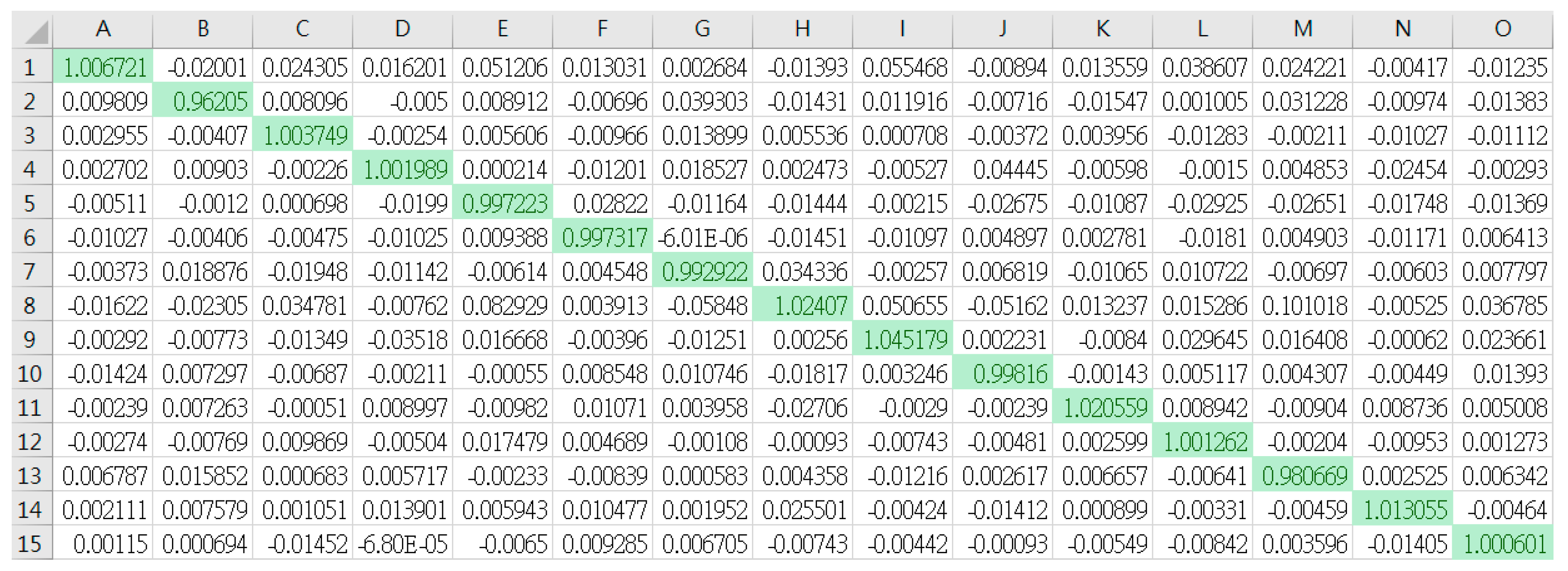
3. Results and Verification

The analysis is mainly carried out by applying a digital MFCC algorithm and using the acoustic sensors. In Figure 4, we establish an experimental structure of our research arrangement process.
Our original information on frog sound is from the digital learning website [27], and their sound information files are shown in Figure 5. Through adjusting pre-emphasis coefficient “ a ”, twenty-five filtered features of each frog are shown in Figure 6.
The MFCC filtering algorithm is applied to the transformation from time-domain signal to special spectrum features as shown in Figure 7. Also, a dataset for training is formed and shown in Figure 8.
When preprocessing is done, the key analysis follows. The feedforward neural networks algorithm is used to train the bioacoustic model datasets of frog. The computation platform we use for conducting the analysis is “MATLAB R2019a-academic use” authorized by National Cheng Kung University, Tainan, Taiwan. And the two processors adopted for classification are GPU and CPU. For each processor, two optimizer functions, “ traingda ” and “ trainscg ”, are executed. Going from the current layers and the next layers of neurons, many comparisons and tests are conducted so that the two processors can learn and attempt to predict an expected model. If the new testing data become the input, this algorithm structure can monitor the data information and predict the classification results by the learning program for training datasets. The calculation of machine learning contains a concept called the “Deep Feedforward Neural Network” method. Furthermore, the “back-propagation algorithm” is used to update the weighting scheme. In the deep learning computation procedure, the back-propagation algorithm will be carried out by iterations not only to minimize the loss function but to get close to the best performance of the testing model. With regard to the optimizer functions, the “ traingda ” (GDA) is a neural network optimizer function that resets the weighting scheme and the bias value based on gradient descent with an adaptive learning rate (LR) for an optimal change in the learning rate during the training process. This can allow the computing condition to keep stable. In short, the “ traingda ” function can automatically alter the LR by adapting to the convergence factor from the error values.
dx = lr × dperf / dx .
Each variable is adjusted according to gradient descent. At each epoch, if performance drops toward the goal, then the LR is increased by the factor “ lr _ inc ”. In contrast, if performance becomes larger than the factor “ max _ perf _ inc ”, the LR is revised down by the factor “ lr _ dec ”. Also, a general fixed learning rate η is then replaced by an adaptive learning rate:
c 1 [ number   of   iterations ] + c 2 .
The “ trainscg ” is a network optimizer function which renovates bias values and weights according to the scaled conjugate gradient (SCG) method. It trains any network as long as its net input, weight, and transfer functions have derivative functions. Backpropagation is used to calculate derivatives of performance “ perf ” with respect to the weights and bias vectors x .
There are three important diagrams from GPU and CPU: Regression, Performance, and Training State. In Regression, the slope (or we can say efficiency), marked as R, of the linear regression shows us the level this machine training is able to achieve. The point of Performance is to see green circle if it can catch up with where the epochs are now. Regarding the Training State, it indicates whether the efficiency of the analysis is going up or down. Basically, we try to improve the accuracy of the classification by changing the training function and processor. The rest of the set of parameters are the same. Related parameters are set up as the learning rate, 0.00008, the initial epoch, 30,000, and the hidden layers being [ 100 ,   200 ,   400 ,   200 ,   100 ] for five layers of neurons.
From Figure 9, Figure 10, Figure 11, Figure 12, Figure 13, Figure 14, Figure 15, Figure 16, Figure 17, Figure 18, Figure 19, Figure 20, Figure 21 and Figure 22, the identified patterns can be categorized into five groups. Figure 9, Figure 10 and Figure 11 report results based on processor GPU with optimizer GDA while Figure 12, Figure 13 and Figure 14 are based on processor CPU with optimizer GDA. Figure 15, Figure 16 and Figure 17 are from processor GPU with optimizer SCG and Figure 18, Figure 19 and Figure 20 are from processor CPU with optimizer SCG. Also, Figure 21 and Figure 22 report the results of the SVM. Additionally, when it comes to the characteristic of GPU, it is commonly thought of as a rapid computation compared with CPU. With regard to computation in MATLAB platform, a GPU does not need too much time to finish the identification. Summary results are shown in Table 1. Comparatively, Table 2 makes the comparison in total time between the feedforward neural network and the support vector machine.
Although the four combinations of processors and optimizers appear to have high and similar R-scores, there still exist some differences. First, due to the adaptive learning rate, optimizer function GDA can adjust the learning rate by itself to approach the best regression. Second, in Figure 10b, it is obvious that the gradient with function GDA goes up and down, appearing to be quite unstable. However, when Figure 10b is compared with Figure 16b, the gradient with function SCG converges more stably, and Figure 10a and Figure 16a confirm the observation. Third, in Figure 10b, the validation check raises dramatically but in Figure 16b it stays almost unchanged, meaning that the GDA function needs more iteration checks to balance the unsteady gradient so that the gradient could converge. Fourth, as shown in Table 1, the total time taken by combinations of process GPU and either of the two optimizers is smaller than that taken by other combinations, suggesting that the computation rate of processor GPU is faster than that of processor CPU. Furthermore, Table 2 compares the total time taken by neural networks with that taken by support vector machine, and the result shows that neural networks take slightly less time than support vector machine.

4. Conclusions

This study applies artificial intelligence (AI) to frog species classification of symmetry of the bioacoustics spectral. The feedforward neural networks structure is key to carry out the feature extraction and effective classification. This research uses the bioacoustic signals and the machine learning method to identify twenty-five frogs. Our study proposes an acoustic signal processing MFCC method and a classification system based on the feedforward neural networks approach.
The proposed method is to perform bioacoustic detection for categorization of animal species and use neural networks equipped with machine learning methods on the basis of training datasets to compute and develop the best model for making meaningful predictions. It is a well-suited way to understand anything that can produce sound. Through bioacoustic detection, making predictions of things that are of primary concern based on voice signals becomes feasible and meaningful. In the long term, once the method is fully developed, it is possible to improve these skills in any field.
The experimental results of this study show that two optimizer functions and two processors could effectively perform predictions and reliable analyses on different frogs. The optimizer function SCG can achieve better identification and classification. In addition, the result of this research indicates that we can directly use original data as input for machine learning. In summary, our study demonstrates that effective machine learning through big data can be reached by using the recurrent neural network (RNN) algorithm of a time-variant method. The AI algorithm helps search for distinctive and interesting features, make meaningful classification, and identify feasible feature models corresponding to various animal bioacoustics conditions.
In the future work, we will try to conduct a similar experiment by using different machine learning methods and algorithms, but the dataset will include thirty-five kinds of frogs. The wavelets algorithm is also a very useful feature extraction tool in frequency domain analysis. However, the new machine learning that the recurrent neural networks (RNN) and long short-term memory work (LSTM) methods bring can be available to apply to nature language identification. In addition to classifying the same animal, it is possible for us to advance the classification process by including many kinds of animals. As the methods of acoustic detection could be used widely, we hope that it can lead to an improvement in the medical field so that we can avoid time-consuming therapies and add some acoustic detection methods to analyze the symptoms more efficiently, such as heartbeat and the sound of flowing blood.

Author Contributions

C.-K.S. and Y.-C.C. generated the research idea, collect related information and assisted in the experiment. K.-W.C. did the experiment, integrated the materials and wrote the article. N.-Z.H. and W.-H.C. technically supported the project, supervised the experiment, polished the whole article and proofread all the details.

Funding

This research received no external funding.

Acknowledgments

The authors would like to thank the website, Frog’s Word (http://learning.froghome.org/), for providing the sound materials for this research.

Conflicts of Interest

The authors declare no conflict of interest.

References

  1. Gretta, T.P.; Miguel, B.A.; Johann, D.B.; Julia, B.; Timothy, C.B.; Chen, I.C.; Timothy, D.C.; Robert, K.C.; Finn, D.; Birgitta, E.; et al. Biodiversity redistribution under climate change: Impacts on ecosystems and human well-being. Science 2017, 355, 9214. [Google Scholar]
  2. Davis, M.B.; Shaw, R.G. Range shifts and adaptive responses to quaternary climate change. Science 2001, 292, 673–679. [Google Scholar] [CrossRef] [PubMed]
  3. Peter, M.N.; Sebastiaan, W.F.M. Climate change and frog calls: Long-term correlations along a tropical altitudinal gradient. Proc. R. Soc. B 2014, 281. [Google Scholar] [CrossRef]
  4. Xie, J.; Towsey, M.; Zhang, J.; Paul, R. Detecting frog calling activity based on acoustic event detection and multi-label learning. Procedia Comput. Sci. 2016, 80, 627–638. [Google Scholar] [CrossRef]
  5. Amalia, L.; Javier, R.L.; Alejandro, C.; Julio, B. Non-sequential automatic classification of anuran sounds for the estimation of climate-change indicators. Expert Syst. Appl. 2018, 95, 248–260. [Google Scholar]
  6. John, J.V.; Colin, T.; Michael, K.; Alex, T.; Joah, M. Applications of machine learning in animal behaviour studies. Anim. Behav. 2017, 124, 203–220. [Google Scholar]
  7. Kelly, R.F.; Matthew, J.S.; Mason, A.P.; Noa, P.W. The use of multilayer network analysis in animal behaviour. Anim. Behav. 2019, 149, 7–22. [Google Scholar]
  8. Xie, J.; Karlina, I.; Lin, S.; Michael, T.; Zhang, J.; Paul, R. Acoustic classification of frog within-species and species-specific calls. Appl. Acoust. 2018, 131, 79–86. [Google Scholar] [CrossRef]
  9. Ahmad, A.; Miad, F. Acoustic signal classification of breathing movements to virtually aid breath regulation. IEEE J. Biomed. Health Inform. 2013, 17, 493–500. [Google Scholar]
  10. Chen, Y.T. An Intelligent Nocturnal Animal Sound Identification System. Master’s Thesis, National Dong Hwa University, Taiwan, July 2011. [Google Scholar]
  11. Amalia, L.; Jesús, G.B.; Alejandro, C.; Julio, B. Exploiting the symmetry of integral transforms for featuring anuran calls. Symmetry 2019, 11, 405. [Google Scholar]
  12. Wu, J.D.; Mingsian, R.B.; Su, F.C.; Huang, C.W. An expert system for the diagnosis of faults in rotating machinery using adaptive order-tracking algorithm. Expert Syst. Appl. 2009, 36, 5424–5431. [Google Scholar] [CrossRef]
  13. Tuomas, V.; Mark, D.P.; Daniel, P.W.E. Computational Analysis of Sound Scenes and Events; Spring International Publishing: Cham, Switzerland, 2017; pp. 303–333. [Google Scholar]
  14. Huang, C.J.; Yang, Y.J.; Yang, D.X.; Chen, Y.J. Frog classification using machine learning techniques. Expert Syst. Appl. 2009, 36, 3737–3743. [Google Scholar] [CrossRef]
  15. Jeffrey, A.N.; Sue, E.M.; Phyllis, J.S. A sound budget for the southeastern Bering Sea: Measuring wind, rainfall, shipping, and other sources of underwater sound. J. Acoust. Soc. Am. 2010, 128, 58–65. [Google Scholar]
  16. Lei, B.; Zhang, Y.; Yang, Y. Detection of sound field aberrations caused by forward scattering from underwater intruders using unsupervised machine learning. IEEE Access 2017, 7, 17608–17616. [Google Scholar] [CrossRef]
  17. Anshul, T.; Daksh, T.; Padmanabhan, R.; Aditya, N. Deep metric learning for bioacoustic classification: Overcoming training data scarcity using dynamic triplet loss. J. Acoust. Soc. Am. 2019, 146, 534–547. [Google Scholar]
  18. Anshul, T.; Padmanabhan, R. Deep archetypal analysis based intermediate matching kernel for bioacoustic classification. IEEE J. Selec. Top. Sign. Process. 2019, 13, 298–309. [Google Scholar]
  19. Juan, J.N.A.; Carlos, M.T.; David, S.R.; Malay, K.D.; Garima, V. Automatic classification of frogs calls based on fusion of features and SVM. In Proceedings of the Eighth International Conference on Contemporary Computing (IC3), Noida, India, 20–22 August 2015. [Google Scholar]
  20. Lincon, S.S.; Bernardo, B.G.; Kazuhiro, F. Classification of bioacoustic signals with tangent singular spectrum analysis. In Proceedings of the IEEE International Conference on Acoustics, Speech and Signal Processing (ICASSP), Brighton, UK, 12–17 May 2019. [Google Scholar]
  21. Stavros, N. Automatic acoustic classification of insect species based on directed acyclic graphs. J. Acoust. Soc. Am. 2019, 145, 541–546. [Google Scholar]
  22. Kirsten, M.P.; Meah, V.L.; Joanne, M.A.N. Frogs call at a higher pitch in traffic noise. Ecol. Soc. 2009, 14, 1–24. [Google Scholar]
  23. Oscar, E.O.; Luis, J.V.R.; Carlos, J.C.B. Variable response of anuran calling activity to daily precipitation and temperature: Implications for climate change. Ecosphere 2013, 4, 1–12. [Google Scholar]
  24. Paul, S.C.; Jeff, H. Designing better frog call recognition models. Ecol. Evol. 2017, 7, 3087–3099. [Google Scholar]
  25. Qian, K.; Zhang, Z.; Alice, B.; Björn, S. Active learning for bird sound classification via a kernel-based extreme learning machine. J. Acoust. Soc. Am. 2017, 142, 1796–1804. [Google Scholar] [CrossRef]
  26. Wang, Y.; Wei, Z.; Yang, J. Feature trend extraction and adaptive density peaks search for intelligent fault diagnosis of machines. IEEE Trans. Ind. Inform. 2019, 15, 105–115. [Google Scholar] [CrossRef]
  27. Frogs’ World. Available online: http://learning.froghome.org/ (accessed on 1 January 2010).
  28. Xie, J.; Michael, T.; Zhang, J.; Paul, R. Frog call classification: A survey. Artif. Intell. Rev. 2018, 49, 375–391. [Google Scholar] [CrossRef]
  29. Xie, J.; Michael, T.; Zhang, J.; Paul, R. Investigation of acoustic and visual features for frog call classification. J. Sign. Process. Syst. 2019. [Google Scholar] [CrossRef]
  30. Marc, G.; Damian, M. Environmental sound monitoring using machine learning on mobile devices. Appl. Acoust. 2020, 159, 107041. [Google Scholar]
  31. Jesús, B.A.; Josué, C.; Rohit, S.; Carlos, M.T.; Federico, B.; Adrián, G.; Alexander, V.; Mark, W. Automatic anuran identification using noise removal and audio activity detection. Expert Syst. Appl. 2017, 72, 83–92. [Google Scholar]
  32. Juan, G.C.; Marco, C.; Mario, S.J.; Eduardo, F.N. An incremental technique for real-time bioacoustic signal segmentation. Expert Syst. Appl. 2015, 42, 7367–7374. [Google Scholar]
  33. Sebastian, R.; Vahid, M. Python Machine Learning, 2nd ed.; Packt Publishing: Birmingham, UK, 2017. [Google Scholar]
  34. Sumeet, D.; Xian, D. Data Mining and Machine Learning in Cybersecurity, 1st ed.; Auerbach Publications: New York, NY, USA, 2011; pp. 7–26. [Google Scholar]
  35. Francesco, C.; Alessandro, V. Machine Learning for Audio, Image and Video Analysis, 2nd ed.; Springer: London, UK, 2015; pp. 99–105. [Google Scholar]
  36. Lindasalwa, M.; Mumtaj, B. Voice recognition algorithms using Mel frequency cepstral coefficient (MFCC) and dynamic time warping (DTW) techniques. J. Comput. 2010, 2, 138–143. [Google Scholar]
  37. Gong, C.A.; Su, C.S.; Chuang, Y.C.; Tseng, K.H.; Li, T.H.; Chang, C.H.; Huang, L.H. Feature extraction of rotating apparatus using acoustic sensing technology. In Proceedings of the 11th International Conference on Ubiquitous and Future Networks, Split, Croatia, 2–5 July 2019. [Google Scholar]
  38. Gopi, E.S. Digital Speech Processing Using Matlab; Springer: Trichy, India, 2013; pp. 105–125. [Google Scholar]
  39. Hiroshi, I. Social Big Data Mining, 1st ed.; CRC Press: Boca Raton, FL, USA, 2015; pp. 125–135. [Google Scholar]
  40. Tobias, G.; Mahmoud, K.; Robert, P.C.; Brian, C.J.M. Using recurrent neural networks to improve the perception of speech in non-stationary noise by people with cochlear implants. J. Acoust. Soc. Am. 2019, 146, 705–718. [Google Scholar]
  41. Sovan, L.; Jean, F.G. Artificial Neuronal Networks: Application to Ecology and Evolution; Springer: Berlin, Germany, 2012; pp. 3–11. [Google Scholar]
  42. James, A.A.; Edward, R. Neurocomputing: Foundations of Research; A Bradford Book; The MIT Press: Cambridge, MA, USA, 1989. [Google Scholar]
  43. Fu, L. Neural Networks in Computer Intelligence; McGraw-Hill Inc.: New York, NY, USA, 1994. [Google Scholar]
  44. Bhavani, T.; Latifur, K.; Mamoun, A.; Wang, L. Design and Implementation of Data Mining Tools, 1st ed.; Auerbach Publications: Boca Raton, FL, USA, 2019. [Google Scholar]
  45. Pan, Y.P.; Liu, Y.Q.; Xu, B.; Yu, H.Y. Hybrid feedback feedforward: An efficient design of adaptive neural network control. Neural Netw. 2016, 76, 122–134. [Google Scholar] [CrossRef]
  46. Dreyfus, G. Neural Neetworks Methodology and Applications; Springer: Berlin/Heidelberg, Germany, 2002. [Google Scholar]
  47. Corinna, C.; Vladimir, V. Support-vector networks. Mach. Learn. 2007, 20, 273–297. [Google Scholar]
  48. Guandong, X.; Zong, Y.; Yang, Z. Applied Data Mining, 1st ed.; CRC Press: Boca Raton, FL, USA, 2013; pp. 112–115. [Google Scholar]
  49. Almo, F. Soundscape Ecology: Principles, Patterns, Methods and Applications; Springer: Dordrecht, The Netherlands; New York, NY, USA, 2014. [Google Scholar]
  50. Gingras, B.; Boeckle, M.; Herbst, C.T.; Fitch, W.T. Call acoustics reflect body size across four clades of anurans. J. Zool. 2012, 289, 143–150. [Google Scholar] [CrossRef]
  51. Gnitecki, J.; Moussavi, Z.M. Separating Heart Sounds from Lung Sounds Accurate Diagnosis of Respiratory Disease Depends on Understanding Noises. IEEE Eng. Med. Biol. Mag. 2007, 6, 20–29. [Google Scholar] [CrossRef] [PubMed]
  52. Daryush, D.M.; Matías, Z.; Feng, S.W.; Harold, A.C.; Robert, E.H. Mobile Voice Health Monitoring Using a Wearable Accelerometer Sensor and a Smartphone Platform. IEEE Trans. Biomed. Eng. 2012, 59, 3090–3096. [Google Scholar]
  53. James, M.G.; Jose, A.G.; Lam, A.C.; Stephen, R.E.; Phil, G.; Roger, K.M.; Edward, H. Restoring speech following total removal of the larynx by a learned transformation from sensor data to acoustics. J. Acoust. Soc. Am. 2017, 141, 307–313. [Google Scholar]
  54. Jacob, B.; Man, M.S.; Huang, Y.A. Springer Handbook of Speech Processing; Springer: Berlin/Heidelberg, Germany, 2008; pp. 161–180. [Google Scholar]
  55. Sandro, S. Introduction to Deep Learning from Logical Calculus to Artificial Intelligence; Springer International Publishing: Berlin, Germany, 2018; pp. 51–119. [Google Scholar]
  56. Marco, A.A.F. Artificial Intelligence Emerging Trends and Applications; Intech: London, UK, 2018; pp. 275–291. [Google Scholar]
  57. Leanne, L. Artificial Intelligence for Fashion: How AI Is Revolutionizing the Fashion Industry, 1st ed.; Apress: New York, NY, USA, 2018; pp. 53–66, 141–144. [Google Scholar]
  58. Mohamed, A.F.; Makhlouf, D.; Mithun, M.; Abdelouahid, D.; Leandros, M.; Helge, J. Blockchain technologies for the internet of things: Research issues and challenges. IEEE Internet Things J. 2019, 6, 2188–2204. [Google Scholar]
  59. Christopher, J.C.B. A Tutorial on Support Vector Machine for Pattern Recognition. Data Min. Knowl. Discov. 1998, 2, 121–167. [Google Scholar]
  60. Pandian, V. Artificial Intelligence Techniques and Algorithms; Baker & Taylor: Charlotte, NC, USA, 2014; pp. 191–192. [Google Scholar]
Figure 1. (a) An ultrasound microphone is equipped to record the sounds from the overall environment; (b) The data acquisition module is used for the microphone to collect real-time signals.
Symmetry 11 01454 g001
Figure 2. The structure of the feedforward neural network approach algorithm is shown. Basically, the structure interprets the general concept of neural networks, which contains layers and layers of neurons. Here, the information flows only in the forward direction from the input to the output in the feedforward neural network approach (FNNA) scheme.
Symmetry 11 01454 g002
Figure 3. The structure of the linear support vector machine algorithm. Generally, this method is used to generate the input-output mapping from training dataset.
Symmetry 11 01454 g003
Figure 4. (a) This structure introduces the experimental process of the frog classification. Briefly, the process includes raw data collection pre-emphasis Mel-scale frequency cepstral coefficient (MFCC) filtering features classification identification results; (b) The diagram indicates the core elements of the procedure in the experiment.
Symmetry 11 01454 g004
Figure 5. The raw data information on fifteen kinds of frogs is presented in four forms. The time length of each raw data is approximately 20 s. (a) The red signal indicates the raw data information of Rhacophorus-taipeianus; the blue one indicates that of Rhacophorus-arvalis; the black one indicates that of Fejervarya-limnocharis; the green one indicates that of Lithobates-catesbeianus; (b) The red signal indicates the raw data information of Babina-adenopleura; the blue one indicates that of Microhyla-ornata; the black one indicates that of Rana-longicrus; the green one indicates that of Hoplobatrachus-rugulosus; (c) The red signal indicates the raw data information of Hylarana-taipehensis; the blue one indicates that of Pelophylax-plancyi; the black one indicates that of Polypedates-megacephalus; the green one indicates that of Pseudoamolops-sauteri; (d) The red signal indicates the raw data information of Odorrana-swinhoana; the blue one indicates that of Rana-okinavana; the black one indicates that of Rana-guentheri.
Symmetry 11 01454 g005aSymmetry 11 01454 g005b
Figure 6. After a filtering process with the value of ‘ a ’ equal to 0.95, the raw data are pre-emphasized, and the filtering results are shown in four forms. (a) The red signal indicates the filtered data information of Rhacophorus-taipeianus; the blue one indicates that of Rhacophorus-arvalis; the black one indicates that of Fejervarya-limnocharis; the green one indicates that of Lithobates-catesbeianus; (b) The red signal indicates the filtered data information of Babina-adenopleura; the blue one indicates that of Microhyla-ornata; the black one indicates that of Rana-longicrus; the green one indicates that of Hoplobatrachus-rugulosus; (c) The red signal indicates the raw data information of Hylarana-taipehensis; the blue one indicates that of Pelophylax-plancyi; the black one indicates that of Polypedates-megacephalus; the green one indicates that of Pseudoamolops-sauteri; (d) The red signal indicates the raw data information of Odorrana-swinhoana; the blue one indicates that of Rana-okinavana; the black one indicates that of Rana-guentheri.
Symmetry 11 01454 g006aSymmetry 11 01454 g006b
Figure 7. It is a spectrum diagram of frog bioacoustic signals through the MFCC algorithm, plotted with 60,000 points for each frog. The MFCC filtering process transforms the original signals into spectra.
Symmetry 11 01454 g007
Figure 8. Twenty-five features of the first frog. The green area is labeled as X _ YY , where X means the number order of frog and YY means the pre-emphasis coefficient ‘ a ’ with only two decimals shown. The orange area shows that each frog has four hundred spectrum feature values.
Symmetry 11 01454 g008
Figure 9. This is the regression results for processor graphics processing unit (GPU) with optimizer function gradient descent adaptive learning rate (GDA). There are four score values which are training score, validation score, test score, and all score. Regardless of the score types, they all appear to approach the Y = T line that indicates the full percent of training correctness.
Symmetry 11 01454 g009
Figure 10. (a) Shows the best validation performance of processor GPU with optimizer function GDA. In addition to the convergence condition of the mean squared error, the green circle also represents whether the training could catch up with the epochs. The same concept with different settings is shown in Figure 13a, Figure 16a and Figure 19a; (b) This is the training state of GPU with the optimizer function GDA. Because of the adaptive learning rate, optimizer function GDA can adjust the learning rate by itself to approach the best regression but it will take a period of time. Besides, the gradient line indicates how quickly it reduces the error and converges to the goal throughout the computation and the same concept can also be seen in Figure 13b, Figure 16b and Figure 19b.
Symmetry 11 01454 g010
Figure 11. The results of frog bioacoustic signal classification through GPU with the optimizer function GDA. The values represent R-scores of frog identifications. The prominent values in green blocks mean that each frog has been identified closely with the actual species, as well as in Figure 14, Figure 17 and Figure 20.
Symmetry 11 01454 g011
Figure 12. The regression results for central processing unit (CPU) with the optimizer function GDA.
Symmetry 11 01454 g012
Figure 13. (a) The best validation performance of CPU with the optimizer function GDA; (b) The training state of CPU with the optimizer function GDA.
Symmetry 11 01454 g013aSymmetry 11 01454 g013b
Figure 14. The results of frog bioacoustic signal classification through CPU with the optimizer function GDA. The values represent R-scores of frog identifications.
Symmetry 11 01454 g014
Figure 15. The regression results for GPU with the optimizer function scaled conjugate gradient (SCG).
Symmetry 11 01454 g015
Figure 16. (a) The best validation performance of GPU with the optimizer function SCG; (b) The training state of GPU with the optimizer function SCG.
Symmetry 11 01454 g016
Figure 17. The results of frog bioacoustic signal classification through GPU with the optimizer function SCG. The values represent R-scores of frog identifications.
Symmetry 11 01454 g017
Figure 18. The regression results for CPU with the optimizer function SCG.
Symmetry 11 01454 g018
Figure 19. (a) The best validation performance of CPU with the optimizer function SCG; (b) The training state of CPU with the optimizer function SCG.
Symmetry 11 01454 g019aSymmetry 11 01454 g019b
Figure 20. The results of frog bioacoustic signal classification through CPU with the optimizer function SCG. The values represent R-scores of frog identifications.
Symmetry 11 01454 g020
Figure 21. The classification result of support vector machine shows that each frog is corresponded to the actual frog species.
Symmetry 11 01454 g021
Figure 22. This is the classification diagram of support vector machine (SVM). Each frog is regarded as a class. By using the nonlinear SVM algorithm, here the first frog is chosen to be the standard point and the other frogs could be classified based on the first frog. The x-axis represents that feature values from twenty-five pre-emphasis “ a ” has selected with 350 points while y-axis shows the classified condition shown as a ratio. Zero ratio indicates the hyperplane. The ratio could give you the relative possibility to identify each frog (ratio in negative sign is just like positive sign).
Symmetry 11 01454 g022
Table 1. Comparisons of results between GPU and CPU.
Machine Learning ProcessorOptimizer FunctionFinal EpochsTotal Time (Second)R-Scores
GPU traingda 12,2349.2280.99798
CPU traingda 9668577.46200.99818
GPU trainscg 1834.32640.99832
CPU trainscg 19111.54900.99800
Table 2. Comparisons of results between neural networks and support vector machine.
Machine Learning AlgorithmTotal Time (Second)R-Scores
Neural networks (conducted by GPU with training function SCG)4.32640.99832
Support vector machine5.14801.00000

