Numerical Solution of Nonlinear Schrödinger Equation with Neumann Boundary Conditions Using Quintic B-Spline Galerkin Method

Abstract

This paper is concerned with the numerical solution of the nonlinear Schrödinger (NLS) equation with Neumann boundary conditions by quintic B-spline Galerkin finite element method as the shape and weight functions over the finite domain. The Galerkin B-spline method is more efficient and simpler than the general Galerkin finite element method. For the Galerkin B-spline method, the Crank Nicolson and finite difference schemes are applied for nodal parameters and for time integration. Two numerical problems are discussed to demonstrate the accuracy and feasibility of the proposed method. The error norms $L_2$, $L_{\infty }$ and conservation laws $I_1, I_2$ are calculated to check the accuracy and feasibility of the method. The results of the scheme are compared with previously obtained approximate solutions and are found to be in good agreement.

1. Introduction and Governing Equation

In this article, quintic B-spline Galerkin finite element method is applied to find the numerical solution of nonlinear Schrödinger (NLS) equation:

$$i{u}_t=-u_{xx}-\alpha {\left|u\right|}^{2}u$$

(1)

Equation (1) is called a self- focusing NLS equation ($\alpha >0$) and allows for bright soliton solutions, as well as the defocusing NLS equation ($\alpha <0$). $u=u\left(x,t\right)$ is a complex-valued function over the real line, $\alpha$ is a positive number and $i$ = $\sqrt{-1}$. The initial and boundary conditions are as follows:

$$u\left(x,0\right)=f\left(x\right),\hspace{1em}a\le x\le b,$$

(2)

$$u\left(a,t\right)=u\left(b,t\right)=u_x\left(a,t\right)=u_x\left(b,t\right)=u_{xx}\left(a,t\right)=u_{xx}\left(b,t\right)=0.$$

(3)

Let

$$u\left(x,t\right)=r\left(x,t\right)+is\left(x,t\right)$$

(4)

where $r\left(x,t\right)$ and $s\left(x,t\right)$ are real functions. Substituting Equation (4) into Equation (1), we obtain the coupled partial differential equations

$$\{\begin{array}{l}{s}_t-r_{xx}=\alpha \left(r^2+s^2\right)r,\\ r_t+s_{xx}=-\alpha \left(r^2+s^2\right)s.\end{array}$$

(5)

Finite element method is a powerful and established method used to approximate the solution of the partial differential equation. Besides finite element method, splines are also very useful to approximate the solution of partial differential equation with piecewise polynomial approximation. A finite element method with B-splines defines a new weighting approximate method and possesses computational advantages of B-splines and finite elements. Spline functions have been applied to develop numerical methods for the solution of nonlinear differential equations [1,2]. The analytical solution of the NLS equation is solved by using the inverse scattering method by Zakharov and Shabat [3]. In 1974, Zakharov and Manakov proved that the NLS equation is completely integrable [4]. Many researchers have worked on the solution of the partial differential equations by using collocation finite element method based on splines.

Spline-based numerical methods have been proposed by many researchers to obtain the numerical solution of nonlinear evolutionary problems. Mittal [5] obtained the numerical solutions of the extended Fisher–Kolmogorov equation using the quintic B-spline collocation method. Saka and Dag [6] presented the Galerkin finite element method based on quartic B-spline functions to obtain the numerical solution of the regularized long-wave (RLW) equation. Gardner [7] proposed the Galerkin finite element method based on cubic B-spline to find the numerical solution of the RLW equation. Dogan [8] presented the Galerkin method based on linear space finite elements to the numerical solution of the RLW equation. Kutluay and Ucar [9] and Saka and Dag [10] found the numerical solution of the coupled Korteweg–de-Vries (KdV) and Korteweg–de-Vries–Burgers (KdVB) equations using the Galerkin finite element method based on quadratic and quartic B-spline functions, respectively.

Gorgulu et al. [11] used exponential B-splines Galerkin finite element method for solving the advection–diffusion equation. They developed a new algorithm by incorporating exponential B-spline functions with the Galerkin finite element method. This method gives satisfactory results. The exponential B-splines Galerkin method is also applied to solve the Burger’s equation and the results are comparable with the quartic B-spline collocation method [2].

There are many non-spline numerical methods developed to solve the NLS equation; some of them are discussed here. Wang et al. [12] proposed a finite difference method using an artificial boundary conditions on an unbounded domain. In this scheme, extrapolation operator is applied to deal with the nonlinear term. Moreover, Barletti et al. [13] presented energy-conserving methods that can confer robustness on the numerical solution. Taleei and Dehghan [14] presented a time-splitting pseudo-spectral domain decomposition method, whereby the original equation is split into linear and nonlinear equations. The Chebyshev pseudo-spectral collocation method is used to solve the linear equation in the spatial dimension and Crank–Nicolson scheme in the temporal dimension. In this study, overlapping multi-domain scheme is chosen. Univariate multi-quadrics (MQ) quasi-interpolation method is developed where the spatial derivatives are calculated from the derivative of the quasi-interpolation.

Some spline-based numerical methods are proposed to solve the NLS equation. Quartic spline approximation and semidiscretization were applied using finite difference method by Sheng et al. [15]. Zlotnik and Zlotnik [16] were the first to implement the finite element method using non-discrete transparent boundary conditions. Naturally, higher-order finite element method is observed to converge faster. The exponential B-spline with collocation method was presented by Ersoy et al. [17]. The Crank–Nicolson scheme is used for time integration and exponential cubic B spline functions for the space integration. Dag [18] proposed a Galerkin finite element method based on quadratic B-spline functions.

In this paper, numerical scheme for the Galerkin method with quintic B-spline is developed to solve the NLS equation. Numerical results are generated and compared with some of the afore-mentioned methods.

This paper is organized as follows. In Section 2, the fundamentals of quintic B-spline Galerkin method are introduced. In Section 3, the initial parameters to find the solutions of the system are calculated. Numerical results and test problems are discussed in Section 4 followed by the conclusion in Section 5.

2. Quintic B-spline Galerkin Method

We consider a mesh $\mathsf{\Pi }$ over the finite domain $\left[a,b\right]$ divided uniformly by grid points $x_k$ with $h=x_k-x_{k-1}, k=1,\dots ,N$. Quintic B-spline function is chosen as the weight and trial function. The quintic B-splines, $B_k\left(x\right)$, $k=-2,\dots ,N+2$ at the grid points $x_k$ forms a basis over the interval $\left[a,b\right]$ as follows [19]:

$$B_k\left(x\right) =\frac{1}{h^5}\{\begin{array}{cc}{p}_1={\left(x-x_{k-3}\right)}^5,\hfill & \hfill x\in \left[x_{k-3},x_{k-2}\right],\\ p_2=p_1-6{\left(x-x_{k-2}\right)}^5,\hfill & \hfill x\in \left[x_{k-2},x_{k-1}\right],\\ p_3=p_2+15{\left(x-x_{k-1}\right)}^5,\hfill & \hfill x\in \left[x_{k-1},x_k\right],\\ p_4=p_3-20{\left(x-x_k\right)}^5,\hfill & \hfill x\in \left[x_k,x_{k+1}\right],\\ p_5=p_4+15{\left(x-x_{k+1}\right)}^5,\hfill & \hfill x\in \left[x_{k+1},x_{k+2}\right],\\ p_6=p_5-6{\left(x-x_{k+2}\right)}^5,\hfill & \hfill x\in \left[x_{k+2},x_{k+3}\right],\\ 0\hfill & \hfill \mathrm{otherwise}.\hfill \end{array}$$

(6)

The global approximate solution, $u_N\left(x,t\right)$, for the NLS equation in Equation (1) is written in terms of the quintic B-spline function as

$$u_N\left(x,t\right)=s_N\left(x,t\right)+r_N\left(x,t\right)={\displaystyle \sum }_{k=-2}^{N+2}{\delta }_k\left(t\right)B_k\left(x\right),$$

(7)

where

$$\begin{gathered} {\delta }_k\left(t\right)={\rho }_k\left(t\right)+{\psi }_k\left(t\right) \\ =\{\begin{array}{c}{s}_N\left(x,t\right)={\displaystyle \sum }_{k=-2}^{N+2}{\rho }_k\left(t\right)B_k\left(x\right),\\ r_N\left(x,t\right)={\displaystyle \sum }_{j=-2}^{N+2}{\psi }_k\left(t\right)B_k\left(x\right).\end{array} \end{gathered}$$

(8)

The functions ${\rho }_k\left(t\right)$ and ${\psi }_k\left(t\right)$ are time-dependent parameters that are determined from the boundary and residual conditions. We make use of a local coordinate transformation

$$\eta =x-x_k, \eta \in \left[0,h\right],$$

The quintic B-spline shape functions in Equation (6) can be defined in term of $\eta$,

$$B_k=\frac{1}{h^5}\{\begin{array}{c}{h}^5-5h^4\eta +10h^3{\eta }^2-10h{\eta }^4-{\eta }^5\\ 26h^5-50h^4\eta +20h^3{\eta }^2+20h^2{\eta }^3-20h{\eta }^4+5{\eta }^5\\ 66h^5-60h^3{\eta }^2+30h{\eta }^4-10{\eta }^5\\ 26h^5+50h^4\eta +20h^3{\eta }^2-20h^2{\eta }^3-20h{\eta }^4+10{\eta }^5\\ {\eta }^5+5h^4\eta +10h^3{\eta }^2+10h^2{\eta }^3+5h{\eta }^4-5{\eta }^5\\ {\eta }^5\end{array}$$

(9)

Since all other quintic B-spline functions are zero over the interval $\left[x_k, x_{k+1}\right]$ except for $B_{k-2}, B_{k-1},\dots ,B_{k+3},$ the approximation function in Equation (8) over the typical interval $\left[x_k, x_{k+1}\right]$ can be written as

$$\begin{gathered} s_N\left(x,t\right)={\displaystyle \sum }_{j=k-2}^{k+3}{\rho }_j\left(t\right)B_j\left(x\right), \\ {r}_N\left(x,t\right)={\displaystyle \sum }_{j=k-2}^{k+3}{\psi }_j\left(t\right)B_j\left(x\right). \end{gathered}$$

(10)

Applying the quintic B-splines definition in Equations (6)–(8), the nodal values of $s_k$, $r_k,$ and its first and second derivatives at the knots $x_k$ are found to be

$$\begin{gathered} s_k=s\left(x_k\right)={\rho }_{k-2}+26{\rho }_{k-1}+66{\rho }_k+26{\rho }_{k+1}+{\rho }_{k+2}, \\ {r}_k=r\left(x_k\right)={\psi }_{k-2}+26{\psi }_{k-1}+66{\psi }_k+26{\psi }_{k+1}+{\psi }_{k+1}, \\ h{s^{\prime }}_k=h{s}^{\prime }\left(x_k\right)=5({\rho }_{k+2}+10{\rho }_{k+1}-10{\rho }_{k-1}-{\rho }_{k-2}), \\ h{r^{\prime }}_k=h{r}^{\prime }\left(x_k\right)=5({\psi }_{k+2}+10{\psi }_{k+1}-10{\psi }_{k-1}-{\psi }_{k-2}), \\ {h}^2{s^{″}}_k=h^2{s}^{″}\left(x_k\right)=20\left({\rho }_{k+2}+2{\rho }_{k+1}-6{\rho }_k+2{\rho }_{k-1}+{\rho }_{k-2}\right), \\ {h}^2{r^{″}}_k=h^2{r}^{″}\left(x_k\right)=20\left({\psi }_{k+1}+2{\psi }_k-6{\psi }_k+2{\psi }_{k-1}+{\psi }_{k-2}\right). \end{gathered}$$

(11)

When using the Galerkin method on Equation (5) with weight function $W\left(x\right)$, the weak form of Equation (5) over the finite interval $\left[x_k, x_{k+1}\right]$ $\left[x_k,x_{k+1}\right]$ is written as

$$\{\begin{array}{c}\underset{x_k}{\overset{x_{k+1}}{{\displaystyle \int }}}\left[W{s}_t+W_x{r}_x-\alpha \left(r^2+s^2\right)Wr\right]dx=0,\\ \underset{x_k}{\overset{x_{k+1}}{{\displaystyle \int }}}\left[W{r}_t-W_x{s}_x+\alpha \left(r^2+s^2\right)Ws\right]dx=0,\end{array}$$

(12)

where

$$z_L=\alpha (r^2+s^2).$$

(13)

By using the weight function $W\left(x\right)$ as quintic B-spline shape functions $B_k$ and inserting the quantities $r_N\left(x, t\right)$ and $s_N\left(x, t\right)$ in Equation (10) into the integral Equation (12) instead of $r\left(x, t\right)$ and $s\left(x, t\right)$

$$\{\begin{array}{c}{\displaystyle \sum _{j=k-2}^{k+3}}\left[\left(\underset{0}{\overset{h}{{\displaystyle \int }}}{B}_i{B}_{\mathrm{j}}d\eta \right)\dot{{\rho }_j}+\left(\underset{0}{\overset{h}{{\displaystyle \int }}}{B^{\prime }}_i{B^{\prime }}_{\mathrm{j}}d\eta \right){\psi }_j-\left(z_L\underset{0}{\overset{h}{{\displaystyle \int }}}{B}_i{B}_{\mathrm{j}}d\eta \right){\psi }_j\right]=0,\\ {\displaystyle \sum _{j=k-2}^{k+3}}\left[\left(\underset{0}{\overset{h}{{\displaystyle \int }}}{B}_i{B}_{\mathrm{j}}d\eta \right)\dot{{\psi }_j}-\left(\underset{0}{\overset{h}{{\displaystyle \int }}}{B^{\prime }}_i{B^{\prime }}_{\mathrm{j}}d\eta \right){\rho }_j+\left(z_L\underset{0}{\overset{h}{{\displaystyle \int }}}{B}_i{B}_{\mathrm{j}}d\eta \right){\rho }_j\right]=0,\end{array}$$

(14)

where $i=j=k-2, k-1,k,k+1,k+2, k+3 \mathrm{and} \mathrm{the} \mathrm{dot} “·”$ $\mathrm{represents}$ the derivative with respect to time t.

The finite element in Equation (14) can be written in matrix form as

$$\{\begin{array}{c}{A}^e{\dot{{\rho }_j}}^e+M^e{\psi }_j{}^e-z_L{C}^e{\psi }_j{}^e=0,\\ A^e{\dot{{\psi }_j}}^e-M^e{\rho }_j{}^e+z_L{C}^e{\rho }_j{}^e=0,\end{array}$$

(15)

where ${\rho }_j={\left({\rho }_{k-2},{\rho }_{k-1},{\rho }_k,{\rho }_{k+1},{\rho }_{k+2}, {\rho }_{k+3}\right)}^T$ and ${\psi }_j={\left({\psi }_{k-2},{\psi }_{k-1},{\psi }_k,{\psi }_{k+1},{\psi }_{k+2}, {\psi }_{k+3}\right)}^T$ are the element parameters. The element matrices $A_{ij}^e$, $M_{ij}^e$ and $C_{ij}^e$ are given by integrals

$$\begin{gathered} A_{ij}^e=\underset{0}{\overset{h}{{\displaystyle \int }}}{B}_i{B}_{\mathrm{j}}d\eta , \\ {M}_{ij}^e=\underset{0}{\overset{h}{{\displaystyle \int }}}{B^{\prime }}_i{B^{\prime }}_{\mathrm{j}}d\eta , \\ {C}_{ij}^e=\underset{0}{\overset{h}{{\displaystyle \int }}}{B}_i{B}_{\mathrm{j}}d\eta , \end{gathered}$$

(16)

where $i, j=k-2, k-1,k, k+1, k+2, k+3$. The element matrices in Equation (16) are calculated as

$$\begin{gathered} A_{ij}^e=\frac{h}{2772}\left[\begin{array}{cccccc}5246& 8937& -6588& -79168& -33258& -1077\\ 8937& 397416& 1558706& 1072186& 121641& 1018\\ -6588& 1558706& 7464456& 6602476& 1072186& 15498\\ -79168& 1072186& 6602476& 7464456& 1558706& 29558\\ -33258& 121641& 1072186& 1558706& 397416& 9113\\ -1077& 1018& 15498& 29558& 9113& 252\end{array}\right] \\ {M}_{ij}^e=\frac{1}{126h}\left[\begin{array}{cccccc}12140& 9710& 36590& -14840& -29735& -2030\\ 9710& 103190& 98630& -151100& -54725& -1250\\ 36590& 98630& 236240& -179420& -151100& -6650\\ -14840& -151100& -179420& 236240& 98630& 2300\\ -29735& -54725& -151100& 98630& 103190& 5255\\ -2030& -1250& -6650& 2300& 5255& 350\end{array}\right] \\ {C}_{ij}^e=\frac{h}{2772}\left[\begin{array}{cccccc}5246& 8937& -6588& -79168& -33258& -1077\\ 8937& 397416& 1558706& 1072186& 121641& 1018\\ -6588& 1558706& 7464456& 6602476& 1072186& 15498\\ -79168& 1072186& 6602476& 7464456& 1558706& 29558\\ -33258& 121641& 1072186& 1558706& 397416& 9113\\ -1077& 1018& 15498& 29558& 9113& 252\end{array}\right] \end{gathered}$$

The values of $z_L$ are obtained by writing $s=\frac{s_k+s_{k+1}}{2}$ and $r=\frac{r_k+r_{k+1}}{2}$ in Equation (13). Using the values of $s_N$ and $r_N$ at the grid points $x_k,$ we obtain

$$\begin{gathered} z_L=\frac{\alpha }{4}\left[{\left({\rho }_{k-2}+27{\rho }_{k-1}+92{\rho }_k+92{\rho }_{k+1}+27{\rho }_{k+2}+{\rho }_{k+3}\right)}^2 \\ \hspace{1em}\hspace{1em}\hspace{1em}\hspace{1em}\hspace{1em}\hspace{1em}\hspace{1em}\hspace{1em}\hspace{1em}\hspace{1em}\hspace{1em}\hspace{1em}\hspace{1em}+{\left({\psi }_{k-2}+27{\psi }_{k-1}+92{\psi }_k+92{\psi }_{k+1}+27{\psi }_{k+2}+{\psi }_{k+3}\right)}^2 \right]. \end{gathered}$$

(17)

Assembling all the elements in Equation (15) leads to the following system:

$$\{\begin{array}{c}A\dot{\rho }+M\psi -C\left(z_L\right)\psi =0,\\ A\dot{\psi }-M\rho +C\left(z_L\right)\rho =0,\end{array}$$

(18)

where $\rho ={\left({\rho }_{-2},{\rho }_{-1}, \dots , {\rho }_k,{\rho }_{k+1}\right)}^T$ and $\psi ={\left({\psi }_{-2},{\psi }_{-1},\dots , {\psi }_k,{\psi }_{k+1}\right)}^T$ are the global element parameters, and $A, M$ and $C\left(z_L\right)$ are the global matrices with generalized kth row given by:

$$\begin{gathered} A=\frac{h}{2772}\left(-1077, -32240, 57971, 2167342, 9737938, 15729242, 9737938, \\ 2167342, 57971, -32240, -1077\right),\hspace{1em}\hspace{1em} \\ M=\frac{1}{126h}\left(-2030,-30985,-76215,-263310, 32805,691350,32805,-263310, \\ -76215, -30985, -2030\right)\hspace{1em}\hspace{1em}\hspace{1em}\hspace{1em}\hspace{1em} \\ \begin{array}{ll}C\left(z_L\right)=\frac{h}{2772}(& -1077z_{1L}, -33258z_{1L}+1018z_{2L}, -79168z_{1L}+121641z_{2L}\\ & +15498z_{3L}, -6588z_{1L}+1072186z_{2L}+1072186z_{3L}\\ & +29558z_{4L}, 8937z_{1L}+1558706z_{2L}+6602476z_{3L}+1558706z_{4L}\\ & +9113z_{5L},5246z_{1L}+397416z_{2L}+ 7464456z_{3L}+7464456z_{4L}\\ & +397416z_{5L}+252z_{6L}, 8937z_{2L}+1558706z_{3L}+ 6602476z_{4L}\\ & +1558706z_{5L}+9113z_{6L}, -6588z_{3L}+1072186z_{4L}+ 1072186z_{5L}\\ & +29558z_{6L},-79168z_{4L}+121641z_{5L}+15498z_{6L}, -33258z_{5L}\\ & +1018z_{6L}, -1077 z_{6L}),\end{array} \end{gathered}$$

(19)

where

$$\begin{gathered} z_{1L}=\frac{\alpha }{4}\left[{\left({\rho }_{k-4}+27{\rho }_{k-3}+92{\rho }_{k-2}+92{\rho }_{k-1}+27{\rho }_k+{\rho }_{k+1}\right)}^2 \\ \hspace{1em}\hspace{1em}\hspace{1em}\hspace{1em}\hspace{1em}\hspace{1em}\hspace{1em}\hspace{1em}\hspace{1em}\hspace{1em}\hspace{1em}+{\left({\psi }_{k-4}+27{\psi }_{k-3}+92{\psi }_{k-2}+92{\psi }_{k-1}+27{\psi }_k+{\psi }_{k+1}\right)}^2 \right], \\ {z}_{2L}=\frac{\alpha }{4}\left[{\left({\rho }_{k-3}+27{\rho }_{k-2}+92{\rho }_{k-1}+92{\rho }_k+27{\rho }_{k+1}+{\rho }_{k+2}\right)}^2 \\ \hspace{1em}\hspace{1em}\hspace{1em}\hspace{1em}\hspace{1em}\hspace{1em}\hspace{1em}\hspace{1em}\hspace{1em}\hspace{1em}\hspace{1em}+{\left({\psi }_{k-3}+27{\psi }_{k-2}+92{\psi }_{k-1}+92{\psi }_k+27{\psi }_{k+1}+{\psi }_{k+2}\right)}^2 \right], \\ {z}_{3L}=\frac{\alpha }{4}\left[{\left({\rho }_{k-2}+27{\rho }_{k-1}+92{\rho }_k+92{\rho }_{k+1}+27{\rho }_{k+2}+{\rho }_{k+3}\right)}^2 \\ \hspace{1em}\hspace{1em}\hspace{1em}\hspace{1em}\hspace{1em}\hspace{1em}\hspace{1em}\hspace{1em}\hspace{1em}\hspace{1em}\hspace{1em}+{\left({\psi }_{k-2}+27{\psi }_{k-1}+92{\psi }_k+92{\psi }_{k+1}+27{\psi }_{k+2}+{\psi }_{k+3}\right)}^2\right], \\ {z}_{4L}=\frac{\alpha }{4}\left[{\left({\rho }_{k-1}+27{\rho }_k+92{\rho }_{k+1}+92{\rho }_{k+2}+27{\rho }_{k+3}+{\rho }_{k+4}\right)}^2 \\ \hspace{1em}\hspace{1em}\hspace{1em}\hspace{1em}\hspace{1em}\hspace{1em}\hspace{1em}\hspace{1em}\hspace{1em}\hspace{1em}\hspace{1em}+{\left({\psi }_{k-1}+27{\psi }_k+92{\psi }_{k+1}+92{\psi }_{k+2}+27{\psi }_{k+3}+{\psi }_{k+4}\right)}^2\right], \\ {z}_{5L}=\frac{\alpha }{4}\left[{\left({\rho }_k+27{\rho }_{k+1}+92{\rho }_{k+2}+92{\rho }_{k+3}+27{\rho }_{k+4}+{\rho }_{k+5}\right)}^2 \\ \hspace{1em}\hspace{1em}\hspace{1em}\hspace{1em}\hspace{1em}\hspace{1em}\hspace{1em}\hspace{1em}\hspace{1em}\hspace{1em}\hspace{1em}+{\left({\psi }_k+27{\psi }_{k+1}+92{\psi }_{k+2}+92{\psi }_{k+3}+27{\psi }_{k+4}+{\psi }_{k+5}\right)}^2\right], \\ {z}_{6L}=\frac{\alpha }{4}\left[{\left({\rho }_{k+1}+27{\rho }_{k+2}+92{\rho }_{k+3}+92{\rho }_{k+4}+27{\rho }_{k+5}+{\rho }_{k+6}\right)}^2 \\ \hspace{1em}\hspace{1em}\hspace{1em}\hspace{1em}\hspace{1em}\hspace{1em}\hspace{1em}\hspace{1em}\hspace{1em}\hspace{1em}\hspace{1em}+{\left({\psi }_{k+1}+27{\psi }_{k+2}+92{\psi }_{k+3}+92{\psi }_{k+4}+27{\psi }_{k+5}+{\psi }_{k+6}\right)}^2\right]. \end{gathered}$$

(20)

Substituting the time derivatives of the parameters $\dot{\rho }$ and $\dot{\psi }$ by the finite difference approximation, $\dot{\rho }=\frac{{\rho }^{n+1}-{\rho }^n}{\mathsf{\Delta }t}$ and $\dot{\psi }=\frac{{\psi }^{n+1}-{\psi }^n}{\mathsf{\Delta }t}$ and parameters $\rho$ and $\psi$ by the Crank–Nicolson method, $\rho =\frac{{\rho }^n+{\rho }^{n+1}}{2}$ and $\psi =\frac{{\psi }^n+{\psi }^{n+1}}{2}$ into Equation (18) yields Equation (21).

$$\{\begin{array}{c}A{\rho }^{n+1}+0.5\Delta t\left(M-C\left(z_L\right)\right) {\psi }^{n+1}=A{\rho }^n-0.5\Delta t\left(M-C\left(z_L\right)\right) {\psi }^n\\ A{\psi }^{n+1}-0.5\Delta t\left(M-C\left(z_L\right)\right) {\rho }^{n+1}=A{\psi }^n+0.5\Delta t\left(M-C\left(z_L\right)\right){\rho }^n \end{array}$$

(21)

where ${\rho }^{n+1}={\left({\rho }_{-2}, {\rho }_{-1}, \dots , {\rho }_{N+2} \right)}^T$ and ${\psi }^{n+1}={\left({\psi }_{-2}, {\psi }_{-1}, \dots , {\psi }_{N+2} \right)}^{\mathrm{T}}$ are unknown parameters. This final system consists of $\left(2N+2\right)$ equations and $\left(2N+10\right)$ unknown’s parameters. To find the unique solution of this system, we need to eliminate parameters ${\rho }_{-2}, {\rho }_{-1}, {\rho }_{N+1}, {\rho }_{N+2}$, ${\psi }_{-2}, {\psi }_{-1}, {\psi }_{N+1}$ and ${\psi }_{N+2}$. Using the following boundary conditions

$$u_x\left(a,t\right)=u_x\left(b,t\right)=u_{xx}\left(a,t\right)=u_{xx}\left(b,t\right)=0,$$

we obtain

$$\begin{gathered} {\rho }_{-2}=-\frac{3}{2}{\rho }_2-5{\rho }_1+\frac{15}{2}{\rho }_0, \\ {\rho }_{-1}=\frac{{\rho }_2}{4}+\frac{3}{2}{\rho }_1-\frac{3}{4}{\rho }_0, \\ {\rho }_{N+1}=\frac{1}{4}{\rho }_{N-2}-\frac{3}{2}{\rho }_{N-1}-\frac{3}{4}{\rho }_{N,} \\ {\rho }_{N+2}=-\frac{3}{2}{\rho }_{N-2}-5{\rho }_{N-1}+\frac{15}{2}{\rho }_{N,} \\ {\psi }_{-2}=-\frac{3}{2}{\psi }_2-5{\psi }_1+\frac{15}{2}{\psi }_0, \\ {\psi }_{-1}=\frac{{\psi }_2}{4} +\frac{3}{2}{\psi }_2{}_1-\frac{3}{4}{\psi }_2, \\ {\psi }_{N+1}=\frac{1}{4}{\psi }_{N-2}-\frac{3}{2}{\psi }_{N-1}-\frac{3}{4}{\psi }_{N,} \\ {\psi }_{N+2}=-\frac{3}{2}{\psi }_{N-2}-5{\psi }_{N-1}+\frac{15}{2}{\psi }_{N.} \end{gathered}$$

(22)

3. The Initial Vectors

The initial parameters ${\rho }^0$ and ${\psi }^0$ can be determined using initial and boundary conditions to solve the system in Equation (21). The approximation can be re-written over the interval $\left[a,b\right]$ at $t=0$ as

$$s_N\left(x,0\right)={{\displaystyle \sum }}_{j=-2}^{N+2}{B}_{\mathrm{j}}\left(x\right){\rho }_j^o \mathrm{and} r_N\left(x,0\right)={{\displaystyle \sum }}_{j=-2}^{N+2}{B}_{\mathrm{j}}\left(x\right){\psi }_j^o,$$

(23)

where all parameters ${\rho }^0$ and ${\psi }^0$ are determined. The functions $s_N$ and $r_N$ are required to satisfy the following relations at the nodal points $x_k$:

$$s_N\left(x_k,0\right)=s\left(x_k,0\right),\hspace{1em}\mathrm{and} r_N\left(x_k,0\right)=r\left(x_k,0\right),\hspace{1em}k=0,1,\dots , N.$$

(24)

A pentadiagonal matrix system is obtained using the conditions in Equation (24). The initial vectors ${\rho }^0$ and ${\psi }^0$ can be calculated from the following matrix equations:

$$\left[\begin{array}{cccccccc}54.00& 60.00& 6.00& & & & & \\ 25.25& 67.50& 26.25& 1.00& & & & \\ 1.00& 26.00& 66.00& 26.00& 1.00& & & \\ & & \ddots & \ddots & \ddots & \ddots & & \\ & & & 1.00& 26.00& 66.00& 26.00& 1.00\\ & & & & 1.00& 26.25& 67.50& 25.25\\ & & & & & 6.00& 60.00& 54.00\end{array}\right]\left[\begin{array}{c}{\rho }^0{}_0\\ {\rho }^0{}_1\\ {\rho }^0{}_2\\ ⋮\\ {\rho }^0{}_{N-1}\\ {\rho }^0{}_N\end{array}\right]=\left[\begin{array}{c}{s}^0{}_0\\ s^0{}_1\\ s^0{}_2\\ ⋮\\ s^0{}_{N-2}\\ s^0{}_{N-1}\\ s^0{}_N\end{array}\right]$$

(25)

$$\left[\begin{array}{cccccccc}54.00& 60.00& 6.00& & & & & \\ 25.25& 67.50& 26.25& 1.00& & & & \\ 1.00& 26.00& 66.00& 26.00& 1.00& & & \\ & & \ddots & \ddots & \ddots & \ddots & & \\ & & & 1.00& 26.00& 66.00& 26.00& 1.00\\ & & & & 1.00& 26.25& 67.50& 25.25\\ & & & & & 6.00& 60.00& 54.00\end{array}\right]\left[\begin{array}{c}{\psi }^0{}_0\\ {\psi }^0{}_1\\ {\psi }^0{}_2\\ ⋮\\ {\psi }^0{}_{N-1}\\ {\psi }^0{}_N\end{array}\right]=\left[\begin{array}{c}{r}^0{}_0\\ r^0{}_1\\ r^0{}_2\\ ⋮\\ r^0{}_{N-2}\\ r^0{}_{N-1}\\ r^0{}_N\end{array}\right]$$

(26)

The above system can be solved by inverting the matrices in MATLAB. The approximate solution of $s_N\left(x,t\right)$ and $r_N\left(x,t\right)$ can be calculated from ${\rho }^n$ and ${\psi }^n$ using Equation (21).

4. Numerical Experiments and Results

Two physical problems, single solitary wave and interaction of two solitary waves, were considered to assess the performance of the proposed method summarized in Equation (22). The performance and accuracy of the approach were tested using the $L_2 \mathrm{and} L_{\infty }$ norms defined as

$$L_2=\Vert u^{exact}-u_N\Vert {}_2=\sqrt{h{\displaystyle \sum }_{k=0}^N{\left|u_k{}^{exact}-{(u_N)}_k\right|}^2},$$

(27)

and

$$L_{\infty }=\Vert u^{exact}-u_N\Vert {}_{\infty }=\underset{0\le k\le N}{\max }\left|u_k{}^{exact}-{(u_N)}_k\right|,$$

(28)

where $u^{exact} \mathrm{and} u_N$ denote the exact and numerical solutions, respectively. Moreover, Equation (1) must satisfy the two conservation laws,

$$\begin{gathered} I_1=\underset{a}{\overset{b}{{\displaystyle \int }}}{\left|u\right|}^{2}dx, \\ {I}_2=\underset{a}{\overset{b}{{\displaystyle \int }}}\left({\left|u_x\right|}^2-\frac{1}{2}\alpha {\left|u\right|}^4\right)dx. \end{gathered}$$

4.1. Problem 4.1 (Single Solitary Wave Solution)

A single solitary wave solution to the NLS equation is given as in [20]:

$$u\left(x,t\right)=\beta \left(\sqrt{\frac{2}{\alpha }}\right)expi\left[\frac{1}{2}Sx-\frac{1}{4}\left(S^2-{\beta }^2\right)t\right]sech\beta \left(x-St\right).$$

(29)

The initial and boundary conditions are taken as $u\left(-20, 0\right)=u\left(20, 0\right)=u_x\left(-20, 0\right)=u_x\left(20, 0\right)=u_{xx}\left(-20, 0\right)=u_{xx}\left(20, 0\right)=0.$

The values of the initial parameters from Equations (25) and (26) are calculated by using the initial and boundary conditions. The values of all parameters were chosen to be $\alpha =2, S=4, \beta =1, h=0.05$, and $\Delta t=0.002, 0.001$. The parameter $S$ represents the speed of the solitary wave whose magnitude depends on the real parameter $\mathsf{\beta }$. The $L_2 \mathrm{and} L_{\infty }$ norms and conservation laws $I_1$ and $I_2$ are tabulated in Table 1 for $\Delta t=0.002$ and Table 2 for $\Delta t=0.001$. It is observed that the norms remain very small. The numerical results obtained by the present scheme are more accurate than the explicit, implicit, and split-step Fourier and other methods [19,21,22].

Table 1. Norms and conservation laws for Problem 4.1. with $\Delta t=0.002, \alpha =2, S=4 \mathrm{and} \beta =1$.

$\mathit{t}$	${\mathit{L}}_{\mathit{\infty }}$	${\mathit{L}}_2$	${\mathit{I}}_1$	${\mathit{I}}_2$
$0.5$	$1.9568\times {10}^{-4}$	$2.7670\times {10}^{-4}$	$1.99983872$	$7.33354808$
$1.0$	$1.9568\times {10}^{-4}$	$2.7670\times {10}^{-4}$	$1.99983872$	$7.33354808$
$1.5$	$1.9568\times {10}^{-4}$	$2.7670\times {10}^{-4}$	$1.99983872$	$7.33354808$
$2.0$	$1.9568\times {10}^{-4}$	$2.7670\times {10}^{-4}$	$1.99983872$	$7.33354808$
$2.5$	$1.9568\times {10}^{-4}$	$2.7725\times {10}^{-4}$	$1.99983871$	$7.33354806$
$3.0$	$6.4457\times {10}^{-4}$	$3.0534\times {10}^{-4}$	$1.99983850$.	$7.33354709$
$3.5$	$4.7627\times {10}^{-3}$	$9.9330\times {10}^{-4}$	$1.99982692$	$7.33349360$

Table 2. Norms and conservation laws for Problem 4.1 with $\Delta t=0.001, \alpha =2, S=4 \mathrm{and} \beta =1$.

$\mathit{t}$	${\mathit{L}}_{\mathit{\infty }}$	${\mathit{L}}_2$	${\mathit{I}}_1$	${\mathit{I}}_2$
0.5	$9.78400\times {10}^{-5}$	$1.3835\times {10}^{-4}$	$1.99991936$	$7.33344071$
1.0	$9.78400\times {10}^{-5}$	$1.3835\times {10}^{-4}$	$1.99991936$	$7.33344071$
1.5	$9.78400\times {10}^{-5}$	$1.3835\times {10}^{-4}$	$1.99991936$	$7.33344071$
2.0	$9.78400\times {10}^{-5}$	$1.3837\times {10}^{-4}$	$1.99991936$	$7.33344071$
2.5	$9.78400\times {10}^{-5}$	$1.3945\times {10}^{-4}$	$1.99991935$	$7.33344069$
3.0	$6.44590\times {10}^{-4}$	$1.8914\times {10}^{-4}$	$1.99991914$	$7.33343971$
3.5	$4.76289\times {10}^{-3}$	$9.6293\times {10}^{-4}$	$1.99990755$	$7.33338623$

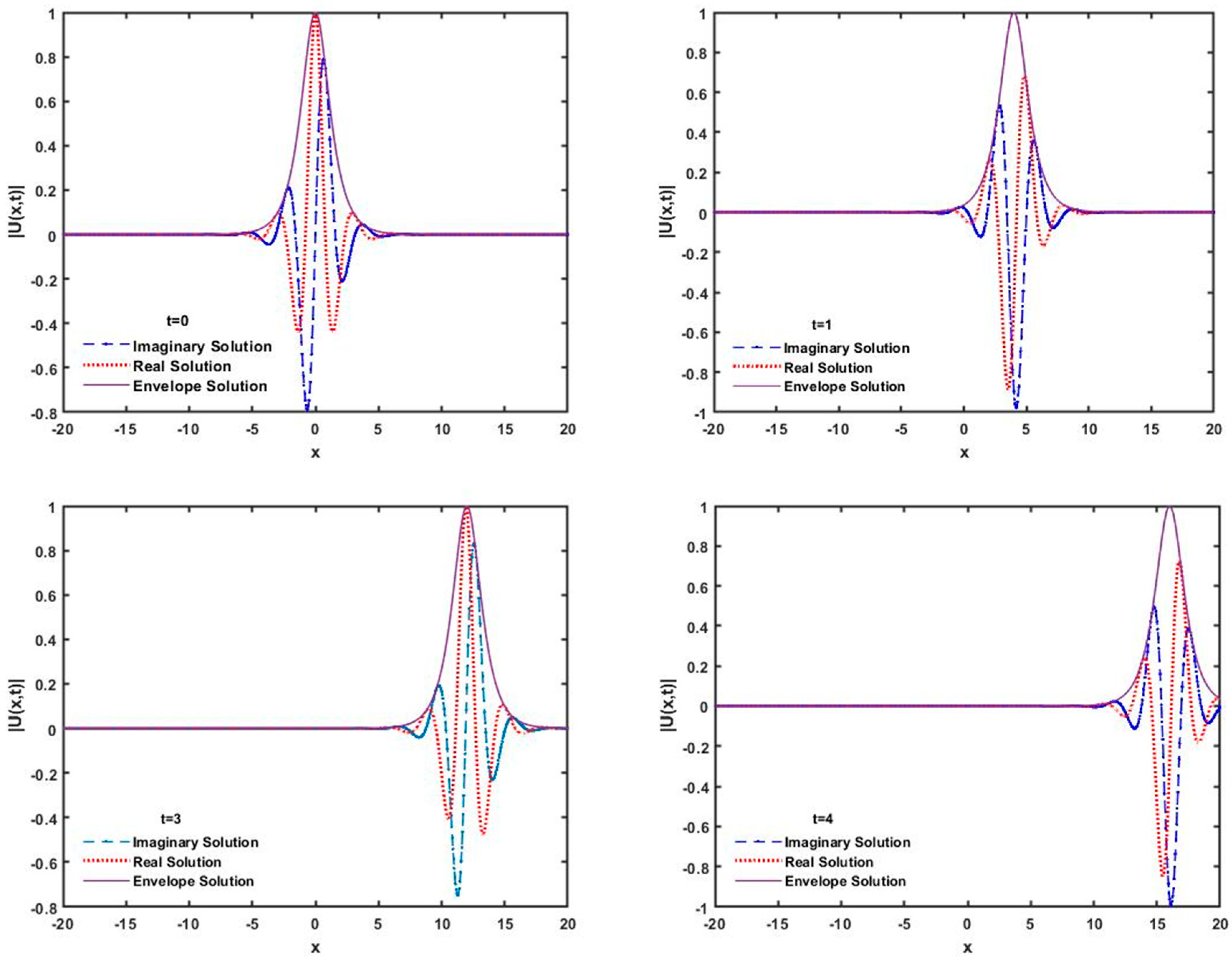
The norms naturally decrease with the increase in number of partitions. We found a good result even for large step size, as displayed in Table 3. The $L_{\infty }$ and $L_2$ norms converge to zero as the number of nodes increases. The numerical simulations are shown at different times over the region $\left[-20, 20\right]$ in Figure 1.

Table 3. Norms and conservation laws for Problem 4.1. with $\Delta t=0.005, \alpha =2, S=4 \mathrm{and} \beta =1 \mathrm{and} t=1$.

$\mathit{h}$	${\mathit{L}}_{\mathit{\infty }}$	${\mathit{L}}_2$	${\mathit{I}}_1$	${\mathit{I}}_2$
0.4000	$3.15055\times {10}^{-3}$	$4.36807\times {10}^{-3}$	$1.99889027$	$7.32694758$
0.3000	$1.93900\times {10}^{-3}$	$2.70993\times {10}^{-3}$	$1.99828775$	$7.32875439$
0.2667	$1.62336\times {10}^{-3}$	$2.28584\times {10}^{-3}$	$1.99826101$	$7.32850737$
0.2500	$1.48026\times {10}^{-3}$	$2.09864\times {10}^{-3}$	$1.99827987$	$7.32841934$
0.2000	$1.11080\times {10}^{-3}$	$1.60406\times {10}^{-3}$	$1.99845175$	$7.32849099$
0.1600	$8.72850\times {10}^{-4}$	$1.27057\times {10}^{-3}$	$1.99869795$	$7.32900596$
0.1333	$7.38540\times {10}^{-4}$	$1.07534\times {10}^{-3}$	$1.99890569$	$7.32957727$
0.1000	$5.95490\times {10}^{-4}$	$8.59430\times {10}^{-4}$	$1.99920350$	$7.33051338$
0.0800	$5.19280\times {10}^{-4}$	$7.42820\times {10}^{-4}$	$1.99939758$	$7.33117069$
0.0667	$4.69970\times {10}^{-4}$	$6.68230\times {10}^{-4}$	$1.99953162$	$7.33163940$
0.0500	$4.04610\times {10}^{-4}$	$5.72190\times {10}^{-4}$	$1.99970290$	$7.33225097$
0.0400	$3.58160\times {10}^{-4}$	$5.05630\times {10}^{-4}$	$1.99980701$	$7.33262780$

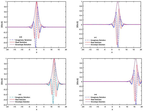
Figure 1. Single solitary wave solution with amplitude 1 and $\Delta t=0.002.$

Furthermore, numerical results for different values of $\Delta t$ were generated to calculate the rate of convergence using the following formula [23]:

$$\mathrm{Order} \mathrm{of} \mathrm{convergence}\approx lo{g}_2\frac{E\left(2h, 2\Delta t\right)}{E\left(h, \Delta t\right)},$$

where $E\left(2h, 2\Delta t\right)$ is either the $L_{\infty }$ error norm or the $L_2$ error norm in spatial and temporal directions. The error norms $L_{\infty }, L_2$ and order of convergence rate at time $t=1$ is shown in Table 4. In Table 4, we see that this method is nearly of second-order convergence.

Table 4. Norms and order of convergence at $t=1$ with $h=\Delta t, \alpha =2, S=4 \mathrm{and} \beta =1.$

$\mathit{h}$	${\mathit{L}}_{\mathit{\infty }}$	Order	${\mathit{L}}_2$	Order
0.040	$3.02045\times {10}^{-3}$	-	$3.0881\times {10}^{-3}$	-
0.020	$7.61510\times {10}^{-4}$	$1.989$	$7.7753\times {10}^{-4}$	$1.9897$
0.010	$1.90750\times {10}^{-4}$	$1.997$	$1.9473\times {10}^{-4}$	$1.9974$
0.005	$4.77100\times {10}^{-5}$	$1.999$	$4.8700\times {10}^{-5}$	$1.9994$

Table 5 presents comparison between our proposed method with other methods. The proposed scheme gave satisfactory results.

Table 5. Comparison of present results for Problem 4.1 with different methods ($\alpha =2, S=4, \beta =1$, $t=1).$

$\mathit{h}$	$\mathbf{\Delta }\mathit{t}$	${\mathit{L}}_{\mathit{\infty }}(\mathbf{Galerkin} \mathbf{Quintic} \mathbf{B}\mathbf{-}\mathbf{spline} \mathbf{Method})$	${\mathit{L}}_{\mathit{\infty }}$ [17,18,19,21,22]
0.0300	0.0050	$4.80\times {10}^{-4}$	$3.00\times {10}^{-4}$
0.0500	0.0010	$1.00\times {10}^{-4}$	$5.77\times {10}^{-3}$
0.0500	0.0050	$5.10\times {10}^{-4}$	$3.00\times {10}^{-4}$
0.0600	0.0165	$1.74\times {10}^{-3}$	$1.50\times {10}^{-3}$
0.3125	0.0200	$8.23\times {10}^{-3}$	$2.00\times {10}^{-3}$
0.3125	0.0026	$1.07\times {10}^{-3}$	$5.13\times {10}^{-3}$

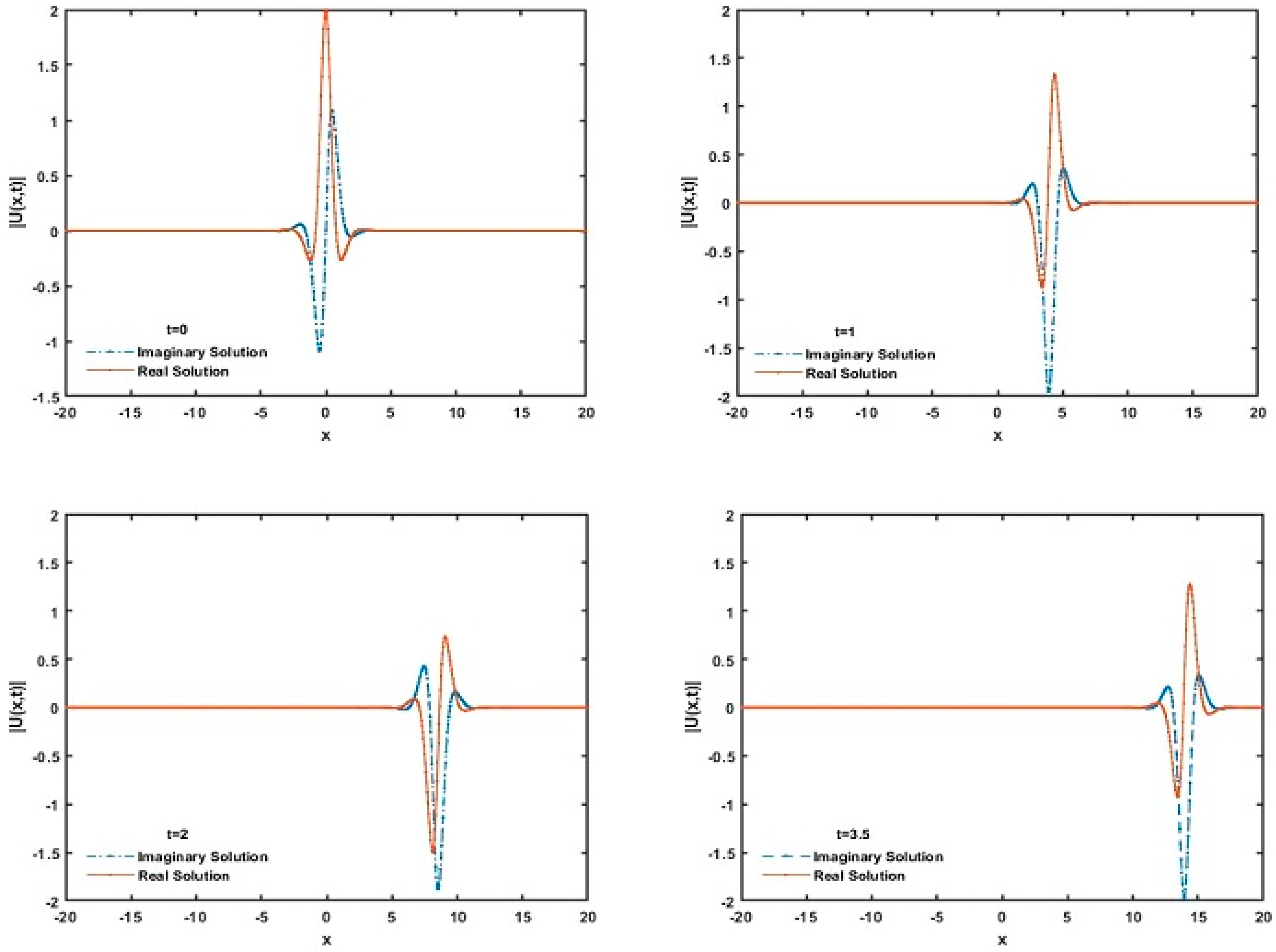
Table 6 displays numerical results of present method compared to those of Taha et al. [21]. In general, the present method generated more accurate results for the specific values of parameters. The simulation of the single soliton with amplitude equal to 2 is presented in Figure 2.

Table 6. Comparison of present results for Problem 4.1 with those of Taha et al. [21] $(\alpha =2, S=4, \beta =2$, $t=1).$

$\mathit{h}$	$\mathbf{\Delta }\mathit{t}$	${\mathit{L}}_{\mathit{\infty }}(\mathbf{Galerkin} \mathbf{Quintic} \mathbf{B}\mathbf{-}\mathbf{spline} \mathbf{Method})$	${\mathit{L}}_{\mathit{\infty }}$ [21]
$0.0300$	$0.00022$	$4.00\times {10}^{-5}$	$7.59\times {10}^{-3}$
$0.1563$	$0.00480$	$1.62\times {10}^{-3}$	$4.64\times {10}^{-3}$
$0.0700$	$0.01200$	$2.31\times {10}^{-3}$	$9.37\times {10}^{-3}$
$0.0600$	0.03000	$5.70\times {10}^{-3}$	$6.95\times {10}^{-3}$
0.0200	0.00040	$7.00\times {10}^{-5}$	$9.63\times {10}^{-3}$
0.0200	0.00010	$2.00\times {10}^{-5}$	$9.31\times {10}^{-3}$

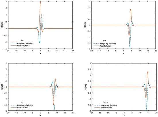
Figure 2. Single solitary wave solution with amplitude 2 and $\Delta t=0.0002.$

4.2. Problem 4.2 (The Interaction of Two Solitary Waves)

In this problem we considered the behavior of two solitons moving in opposite directions using the following initial conditions [18,20,21]:

$$\begin{gathered} u\left(x,0\right)={\displaystyle \sum }_{k=1}^2{u}_k\left(x,0\right), \\ {u}_k\left(x,0\right)={\beta }_k\left(\sqrt{\frac{2}{\alpha }}\right)exp\left(i\left[\frac{1}{2}S\left(x-x_k\right)\right]\right)sech\left({\beta }_k\left(x-x_k\right)\right). \end{gathered}$$

(30)

where ${\beta }_k, \alpha$ and $x_k$ are constants.

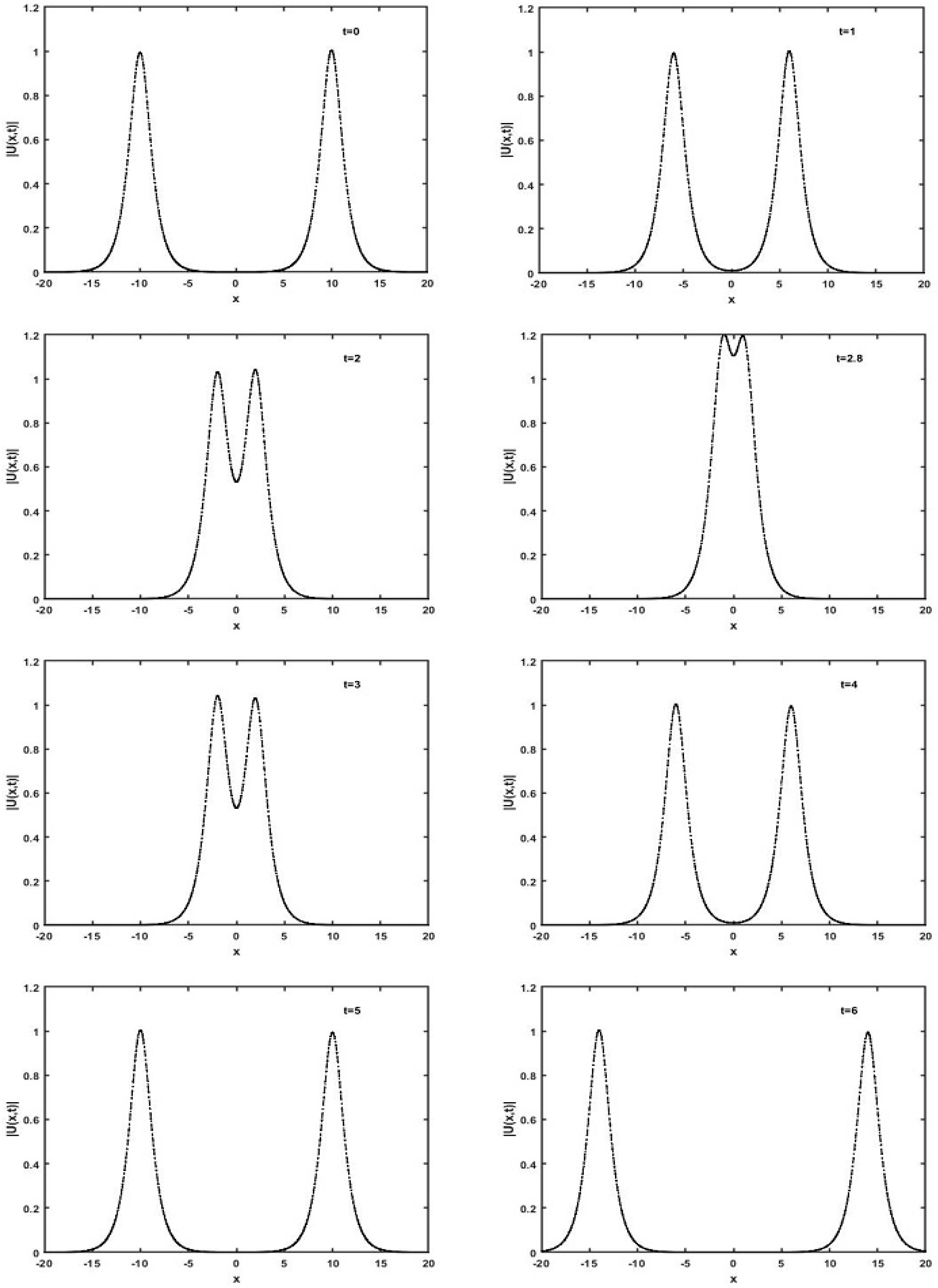
The values of all parameters were chosen to be $x_1=10, x_2=-10, \alpha =2, {\beta }_1=1, {\beta }_2=1, S_1=-4,{ S}_2=4,h=0.05$ and $\Delta t=0.05$. Two solitary waves were traveling in opposite direction with the same magnitude 1 and speed 10. One of the solitary waves placed at $x=10$ was traveling to the left side with speed 4 and the second wave on the other side placed at $x=-10$ was traveling to the right side with speed 4. As we know, solitons move in opposite direction and they collide and separate. We noticed that the shape of the solitons did not change after the collision of both solitons as expected. The two solitary waves collided at times $t=1, 2,3$ and then separated at $t=4, 5, 6$. We see that the solitons preserved the original shapes after the collision. The interactions of two solitons at different times $t=0,1, 2,2.8, 3, 4$, 5 and 6 can be seen in Figure 3.

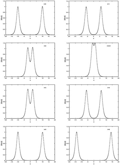
Figure 3. Interaction of two-solitons at different times with amplitude = 1, $\alpha =2$ and $\Delta t=0.0005.$

The $L_{\infty }$ and $L_2$ norms and $I_1$ conservation law were calculated at various times with $\Delta t=0.005, 0.002,$ as shown in Table 7 and Table 8.

Table 7. Norms and conservation laws for Problem 4.2 with $h=0.05 \mathrm{and} \Delta t=0.005.$

$\mathit{t}$	${\mathit{L}}_{\mathit{\infty }}$	${\mathit{L}}_2$	${\mathit{I}}_1$
$0.5$	$4.7310\times {10}^{-4}$	$6.8455\times {10}^{-4}$	$4.00001440$
$1.0$	$4.7310\times {10}^{-4}$	$6.8455\times {10}^{-4}$	$4.00058985$
$1.5$	$4.7277\times {10}^{-4}$	$6.8398\times {10}^{-4}$	$4.02146973$
$2.0$	$4.5716\times {10}^{-4}$	$6.5569\times {10}^{-4}$	$4.58630524$
$2.5$	$9.4000\times {10}^{-7}$	$8.5000\times {10}^{-7}$	$7.99999602$
$3.0$	$4.5739\times {10}^{-4}$	$6.5569\times {10}^{-4}$	$4.58628884$
$3.5$	$4.7280\times {10}^{-4}$	$6.8398\times {10}^{-4}$	$4.02146948$
$4.0$	$4.7310\times {10}^{-4}$	$6.8454\times {10}^{-4}$	$4.00058984$
$4.5$	$4.7310\times {10}^{-4}$	$6.8455\times {10}^{-4}$	$4.00001440$
$5.0$	$4.7310\times {10}^{-4}$	$6.8455\times {10}^{-4}$	$4.00000032$

Table 8. Norms and conservation laws for Problem 4.2 with $h=0.05 \mathrm{and} \Delta t=0.002$.

$\mathit{t}$	${\mathit{L}}_{\mathit{\infty }}$	${\mathit{L}}_2$	${\mathit{I}}_1$
$0.5$	$1.8921\times {10}^{-4}$	$2.7382\times {10}^{-4}$	$4.00001440$
$1.0$	$1.8921\times {10}^{-4}$	$2.7382\times {10}^{-4}$	$4.00058985$
1.5	$1.8908\times {10}^{-4}$	$2.7359\times {10}^{-4}$	$4.02146966$
$2.0$	$1.8289\times {10}^{-4}$	$2.6227\times {10}^{-4}$	$4.58630039$
$2.5$	$1.5000\times {10}^{-7}$	$1.4000\times {10}^{-4}$	$7.99999936$
$3.0$	$1.8293\times {10}^{-4}$	$2.6227\times {10}^{-4}$	$4.58629383$
$3.5$	$1.8909\times {10}^{-4}$	$2.7359\times {10}^{-4}$	$4.02146956$
$4.0$	$1.8921\times {10}^{-4}$	$2.7382\times {10}^{-4}$	$4.00058984$
$4.5$	$1.8921\times {10}^{-4}$	$2.7382\times {10}^{-4}$	$4.00001440$
$5.0$	$1.8921\times {10}^{-4}$	$2.7382\times {10}^{-4}$	$4.00000032$

Furthermore, Table 9 presents numerical results of our proposed method compared with previous methods (e.g., [21]). The present method gives accurate results for the specific values of parameters.

Table 9. Comparison of present results for Problem 4.2 with those of Taha et al. [21]. $\left(amplitude=1\right).$

$\mathit{t}$	$\mathit{h}$	$\mathbf{\Delta }\mathit{t}$	${\mathit{L}}_{\mathit{\infty }}(\mathbf{Galerkin} \mathbf{Quintic} \mathbf{B}\mathbf{-}\mathbf{spline} \mathbf{Method})$	${\mathit{L}}_{\mathit{\infty }}$ [21]
$1.0$	$0.0500$	$0.0025$	$2.36520\times {10}^{-4}$	$9.60\times {10}^{-4}$
$1.0$	$0.0500$	$0.0010$	$9.46000\times {10}^{-5}$	$1.41\times {10}^{-3}$
$1.0$	$0.6250$	$0.0071$	$3.85612\times {10}^{-3}$	$1.22\times {10}^{-3}$
$1.0$	$0.1300$	$0.0036$	$8.44010\times {10}^{-4}$	$1.41\times {10}^{-3}$
$1.6$	$0.0500$	$0.0010$	$9.4460\times {10}^{-5}$	$1.73\times {10}^{-4}$
$1.8$	$0.0700$	$0.0700$	$9.15408\times {10}^{-3}$	$1.58\times {10}^{-3}$

5. Conclusions

In this paper, the numerical solution of the NLS equation with Neumann boundary conditions is obtained by the Galerkin finite element method with quintic B-spline shape function. The accuracy and feasibility of the method was evaluated by two test problems related to single solitary wave and interaction of two solitary waves. The accuracy of numerical method was examined by showing reasonably small error norms $L_2$ and $L_{\infty }$. The interaction of two solitary waves was investigated and observed that the shape of the solitons did not change after the collision of both solitons as expected. The proposed method successfully simulated the soliton picture by choosing different parameters in the case of motion of single soliton and interaction of two soliton. The obtained results were compared with published results [17,19,21,22] and it was observed that the all results are acceptable and reflect the analytical solution. The rate of convergence was calculated and found to be almost of second-order convergence. In conclusion, the present Galerkin finite element scheme with quintic B-spline presents an acceptable soliton solution method for solving NLS equation. The simplicity of the quintic B-spline Galerkin finite element method is an advantage over the general Galerkin finite element method to obtain the numerical solution of NLS equation. The proposed scheme can easily be applied to solve various nonlinear differential equations.

References

- Krowiak, A. Symbolic computing in spline-based differential quadrature method. Commun. Numer. Meth. Eng. 2006, 22, 1097–1107. [Google Scholar] [CrossRef]
- Saka, I.D. Quartic B-spline collocation method to the numerical solutions of the Burgers equation. Chaos Solitons Fracts 2007, 32, 1125–1137. [Google Scholar] [CrossRef]
- Zakharov, V.E.; Shabat, A.B. Exact theory of two dimensional two dimensional self focusing and one dimensional self waves in nonlinear media. Sov. J. Exp. Theor. Phys. 1972, 34, 62–69. [Google Scholar]
- Zakharov, V.E.; Manakov, S.V. On the complete integrability of a nonlinear Schrödinger equation. Theor. Math. Phys. 1974, 19, 332–343. [Google Scholar] [CrossRef]
- Mittal, R.C.; Arora, G. Quintic B-spline collocation method for numerical solution of the extended fisher-kolmogorov equation. Int. J. Appl. Math. Mech. 2010, 6, 74–85. [Google Scholar]
- Saka, I.D. A numerical solution of the RLW equation by Galerkin method using quartic B-splines. Commun. Numer. Methods Eng. 2008, 24, 1339–1361. [Google Scholar] [CrossRef]
- Gardner, L.R.T.; Gardner, G.A. Solitary waves of the regularized long wave equation. J. Comput. Phys. 1990, 91, 441–459. [Google Scholar] [CrossRef]
- Dogan, A. Numerical solution of RLW equation using linear finite elements within Galerkin’s method. Appl. Math. Model. 2002, 26, 771–783. [Google Scholar] [CrossRef]
- Kutluay, S.; Ucar, Y. A quadratic B-spline galerkin approach for solving a coupled KDV equation. Math. Model. Anal. 2013, 18, 103–121. [Google Scholar] [CrossRef]
- Saka, B.; Dag, I. Quartic B-spline Galerkin approach to the numerical solution of the KDVB equation. Appl. Math. Comput. 2009, 215, 746–758. [Google Scholar] [CrossRef]
- Gorgulu, M.Z.; Dag, I. Galerkin method for the numerical solution of the advection-diffusion equation by using exponential B-splines. arXiv, 2016; arXiv:1604.04267v1. [Google Scholar]
- Wang, B.; Liang, D. The finite difference scheme for nonlinear Schrödinger equations on unbounded domain by artificial boundary conditions. Appl. Numer. Math. 2018, 128, 183–204. [Google Scholar] [CrossRef]
- Barletti, L.; Brugnano, L.; Caccia, G.F.; Iavernaro, F. Energy-conserving methods for the nonlinear Schrödinger equation. Appl. Math. Comput. 2018, 318, 3–18. [Google Scholar] [CrossRef]
- Taleei, M.D. Time-splitting pseudo-spectral domain decomposition method for the soliton solutions of the one- and multi-dimensional nonlinear Schrödinger equations. Comput. Phys. Commun. 2014, 185, 1515–1528. [Google Scholar] [CrossRef]
- Sheng, Q.; Khaliq, A.Q.M.; Al-Said, E.A. Solving the generalized nonlinear Schrodinger equation via quartic spline approximation. J. Comput. Phys. 2001, 166, 400–417. [Google Scholar] [CrossRef]
- Zlotnik, A.; Zlotnik, I.A. Finite element method with discrete transparent boundary conditions for the time-dependent 1D schrödinger equation. Kinet. Relat. Models 2012, 5, 639–663. [Google Scholar] [CrossRef]
- Ersoy, I.D.; Sahin, A. Numerical investigation of the solution of Schrodinger equation with exponential cubic B-spline finite element method. arXiv, 2016; arXiv:1607.00166v1. [Google Scholar]
- Dag, I. A quadratic B-spline finite element method for solving nonlinear Schrodinger equation. Comput. Methods Appl. Mech. End Eng. 1999, 174, 247–258. [Google Scholar]
- Saka, B. A quintic B-spline finite-element method for solving the nonlinear Schrödinger equation. Phys. Wave Phenom. 2012, 20, 107–117. [Google Scholar] [CrossRef]
- Gardner, L.R.T.; Gardner, G.A.; Zaki, S.I.; Sahrawi, Z.E. B-spline finite element studies of the non-linear Schriidinger equation. Comput. Methods Appl. Mech. Eng. 1993, 108, 303–318. [Google Scholar] [CrossRef]
- Taha, T.R.; Ablowitz, M.J. Analytical and numerical aspects of certain nonlinear evolution equations II: Numerical, nonlinear Schrodinger equations. J. Comput. Phys. 1984, 55, 203–230. [Google Scholar] [CrossRef]
- Prenter, P. Splines and Variational Methods; Wiley: New York, NY, USA, 1975. [Google Scholar]
- Qu, W.; Liang, Y. Stability and convergence of the Crank-Nicolson scheme for a class of variable-coefficient tempered fractional diffusion equations. Adv. Differ. Equ. 2017, 2017, 108. [Google Scholar] [CrossRef]
© 2019 by the authors. Licensee MDPI, Basel, Switzerland. This article is an open access article distributed under the terms and conditions of the Creative Commons Attribution (CC BY) license (http://creativecommons.org/licenses/by/4.0/).