A Two-Dimensional Mathematical Model of Heat Propagation Equations and Their Significance for Soil Temperature

Abstract

In the context of the development of the research project (Boulaaras et al.) which was supported by the Deanship of Scientific Research of Qassim University under the Project No. 1140 during the academic year 2016/1437, this research will introduce a two dimensional mathematical model based on the finite elements spatial method combined with a finite differences time scheme applied to the diffusion equations. This model will be applied in the hypothetical example where the obtained results will be compared with the real experimental data. Such a comparison will allow to predict the soil temperature for different depths and at different time periods according to certain conditions on the weather and take into account the stability conditions of the used numerical method. It’s worthy of note that some of the concreted mathematical problems will be addressed by the experimental scientific theories of functional analysis and then the numerical simulation of the theoretical study will be provided thanks to sophisticated methods with more convergence and stability. This mathematical model would be reduced by means of physical measurement and also in charge of the physical cost.

1. Introduction

In the recent years, many alternative methods have been used to speed up solving partial differential equations explaining natural phenomena. At this regard, Galerkin methods are being used instead of finite difference style methods to resolve the horizontal and vertical fields in numerical model. These methods can be used to solve partial differential systems and the problems of free border as presented in [1,2,3,4,5,6,7], but so far, such works do not use this method directly in the field of values of grid points after the scale partition. Therefore, no improvements was held concerning the accuracy of the solutions of the ordinary differential equation systems. The processes adopted in solving such systems basically consists of two methods: The finite element method, and the spectral method. Finite element method is a numerical method relies on principles inherited from the weak formulation, which implements a discreet mathematical algorithm aiming to find an approximate solution to the problem of free boundary (see [8,9,10]), and well known as Dirichlet conditions or Neumann data. The method of finite elements differs from the spectral method because it is not exhaustive; it allows instead to specify local values. However, it is a specific approximate function defined throughout the region and not just at distinct points (see [11,12,13,14,15,16,17,18,19,20]).

In fact, numerical methods can be used to solve complicated and unsolvable problems by analytical methods. The use of numerical solutions is limited in terms of the relative errors that must appear after doing a given numbers of iterations in the numerical calculations, and which must be estimated on an appropriate way to judge the acceptance or the rejection of the obtained results. Moreover, the numerical method raises questions about the proposed division such as the convergence and the stability of the method in order to ensure the existence and the uniqueness of the solutions of the studied problem. The numerical analysis relies on the description of the methods, which may allow obtaining numerical solutions to mathematical issues that are usually difficult to be solved by the usual analytical methods. On some issues, we cannot find solutions set by direct analytical methods and conventional theories. In such cases we look for algorithms of specific numerical methods to get the almost exact solutions in given points. Computational modeling can provide a very easy way to predict, and in many cases, can significantly reduce the required amount of field testing. The development of a two-dimensional and three-dimensional model which can be applied to some evolutionary partial equations during the second half of the twentieth century, drew on a continuous progress through automated calculation tools based on classical numerical methods such as finite differences.

In this context, and given that the exact analytic solutions are difficult to be obtained, or indeed do not exist, modern numerical methods, such as the finite elements method, are being applied to some diffusion equations describing the behavior of the soil temperature for different depths and at different day-times according to certain conditions on the weather. Thus, the finite element method, which is falling into a more general Galerkin family method, will be applied along this work to solve such diffusion equations in two-dimension case. The method should take into account the stability conditions of the used numerical method, where the expected values are determined from the initial known values through the observations of the temperature source. The computational model of the transport equations consists of two main steps: The first is to present the equation system that governs the behavior of the continuous temperatures in the soil. The second step is to supersede the equations on the continuous variables with equations involving a separate variable of its solution, obtained by an appropriate algorithm. Moreover, we aim into this research to highlight the application of the method to parabolic equation.

The outline of the paper is as follows: In the first section, some necessary notations of the problem by means of detailed finite element methods description are introduced, where the numerical analysis of the heat equations is studied in order to get the weak formulation of the presented problem using the finite deference time scheme combined with Galerkin method. Then, we establish the stability analysis of the given schemes. In the second section, a two-dimensional numerical prediction model that predicts the temperature field for different depths of homogeneous soil and for different times as well as days is presented. By using the finite element approximation of the Lagrange polynomial of order 1, it will be possible to check the effects of the different parameters governing the physics phenomena as well as the effects of the soil characteristics. And finally, we perform experimental measurements of the ground soil temperature in Qassim province in Kingdom of Saudi Arabia which will be used as real data in order to prove the accuracy of the presented numerical method.

2. Finite Element Methods

2.1. Finite Element Methods Description

The finite element method can be defined on $\widehat{T}\subset {\mathbb{R}}^P$ by a set of $n_d$ nodes $a^i$ and corresponding base functions

$${\widehat{\phi }}^i:\widehat{T}\subset {\mathbb{R}}^p\to {\mathbb{R}}^Q$$

Each base function corresponds to a degree of freedom (dof). most of finite element methods are scalar, which means that $Q=1$ but GETFEM$++$ support also intrinsic vectorial elements. The map between the reference element and the real element is called geometric transformation and is denoted by

$$\tau :\widehat{T}\to T$$

This map is supposed to be polynomial (see [1,13]). The base functions ${\widehat{\phi }}^i$ defined on the reference element define a set of base functions on the real element defined by

$${\tilde{\phi }}^i\left(x\right)={\widehat{\phi }}^i\left(\widehat{x}\right)={\widehat{\phi }}^i\left({\tau }^{-1}\left(x\right)\right)$$

If the element is said to be equivalent through the geometric transformation $\tau$ (or $\tau$-equivalent) then the base functions on the real element are just defined by

$${\phi }^i\left(x\right)={\tilde{\phi }}^i\left(x\right)$$

This is generally the case for Lagrange elements, but not for Hermite elements (when some dof represent the gradient of the unknown). When the element is not equivalent through the geometric transformation then GETFEM$++$ allows to define a square matrix $\tilde{M}$ depending on the real element (i.e., on the geometric transformation) such that base functions on the real element are defined by

$${\phi }^i\left(x\right)=\sum _{j=0}^{n_d-1}{\tilde{M}}_{ij}{\tilde{\phi }}^j\left(x\right)$$

We denote by

$$\left[\widehat{\phi }\left(\widehat{x}\right)\right]=\left(\begin{array}{c}{\widehat{\phi }}^0\left(\widehat{x}\right)\\ {\widehat{\phi }}^1\left(\widehat{x}\right)\\ ⋮\\ {\widehat{\phi }}^{n_d-1}\left(\widehat{x}\right)\end{array}\right)$$

the $n_d\times Q$ matrix, such that when a function is defined by

$$f\left(x\right)=\sum _{i=0}^{n_d-1}{\alpha }_i{\phi }^i\left(x\right)$$

One has

$$f\left(\tau \left(\widehat{x}\right)\right)={\alpha }^T\tilde{M}\left[\widehat{\phi }\left(\widehat{x}\right)\right]$$

where $\alpha$ is the vector of the components ${\alpha }_i$.

2.1.1. Different Types of d.o.f

To each base function of a finite element method corresponds a degree of freedom (d.o.f.) which is a linear form on this function.

Table 1. Most significant types of d.o.f.

Type	Expression	Commentary
Lagrange type	$\mathsf{\Phi }\left(a_i\right)$	Value of $\mathsf{\Phi }$ on the node $\left(a_i\right)$. The most simple d.o.f. allows the Lagrange interpolation
Hierarchical Lagrange Type	$\mathsf{\Phi }\left(a_i\right)-...$	Difference between the value of $\mathsf{\Phi }$ on the node $\left(a_i\right)$ and the value of some other base functions. This is generally the bubble functions type of d.o.f.
Mean type	$\frac{1}{\left|T\right|}{\int }_T\mathsf{\Phi }\left(x\right)dx$	Value of the mean value of $\mathsf{\Phi }$ on the element. Exists also for the restriction on a face
Derivative type	$\frac{\partial }{\partial x_i}\mathsf{\Phi }\left(a_i\right)$ or $\frac{\partial }{\partial \eta }\mathsf{\Phi }\left(a_i\right)$	Value of a derivative of $\mathsf{\Phi }$ on the node $\left(a_i\right)$. This kind of d.o.f. makes the element no to be $\tau$-equivalent. $\frac{\partial }{\partial \eta }\mathsf{\Phi }\left(a_i\right)$ denotes the normal derivative with respect to a face
Second derivative	$\frac{{\partial }^2}{\partial x_i\partial x_j}\mathsf{\Phi }\left(a_i\right)$	Value of a second derivative of $\mathsf{\Phi }$ on the node $\left(a_i\right)$. This kind of d.o.f. makes also the element no to be $\tau$-equivalent.

gives the most significant types of d.o.f.

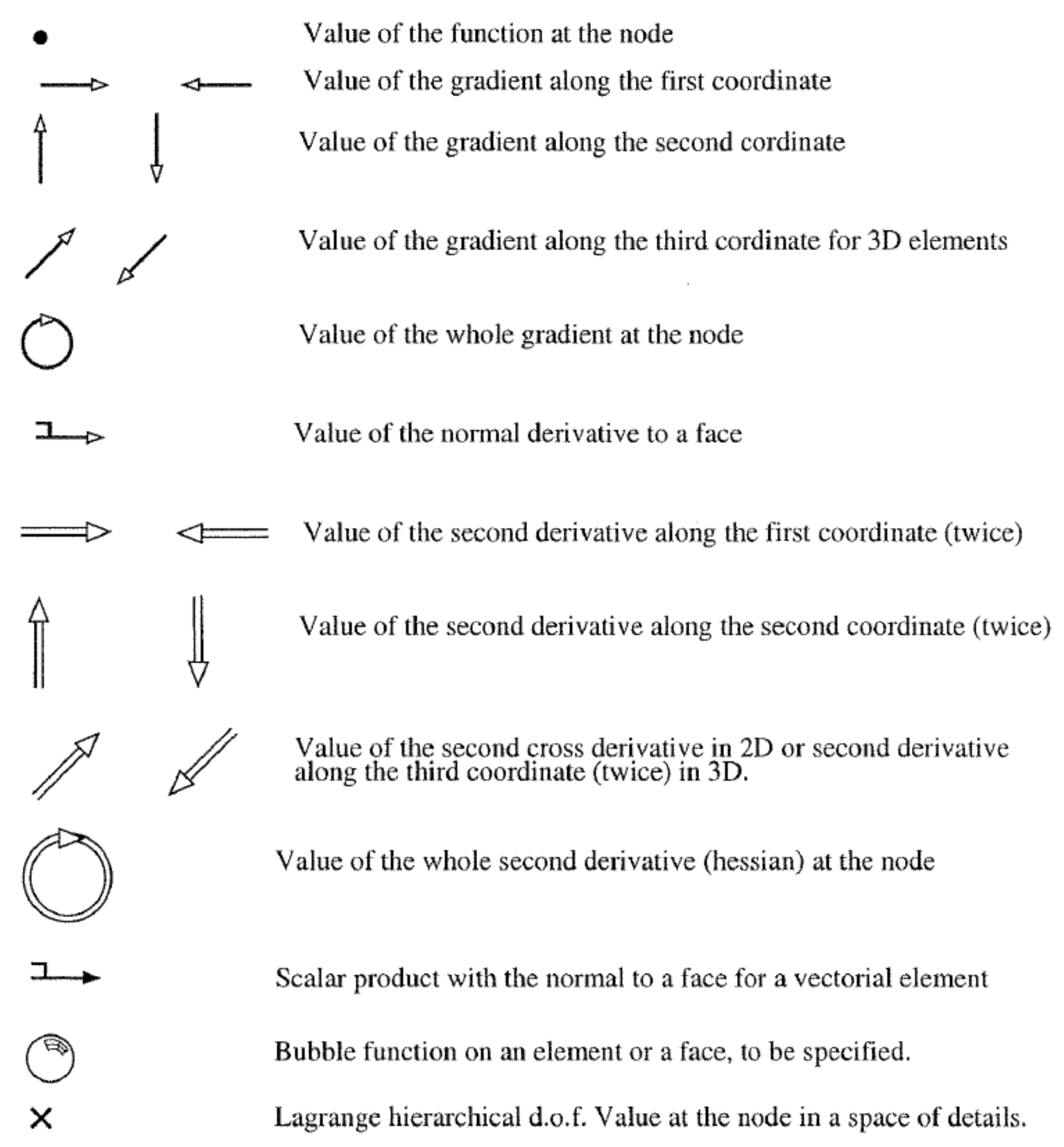
2.1.2. Graphical Codification of d.o.f

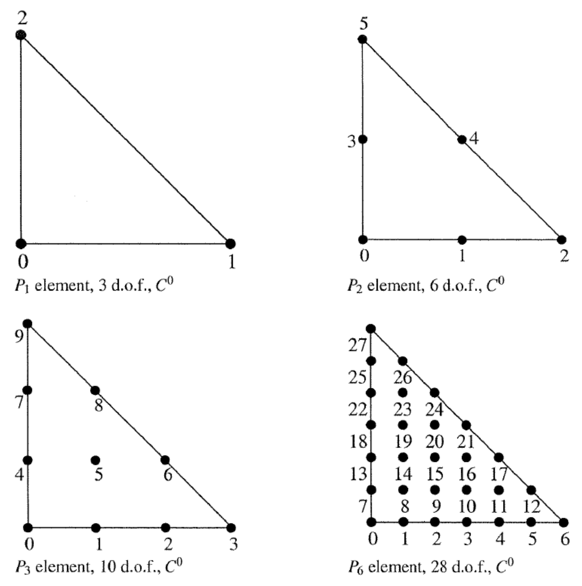
The graphical codification of d.o.f can be defined as shown in Figure 1.

2.2. Classical $P_K$ Lagrange Elements on Simplifies

We can define a classical $P_K$ Lagrange element of qualitative dimension and qualitative, degree. This element has only degrees of freedom wich corresponds to the value of the function on a node. The grid of node is the so-called Lagrange grid. Figure 2, Figure 3 and Figure 4 show examples of dimension 1, 2 and 3.

The degree number of freedom for a classical $P_K$ Lagrange element of dimension P and degree K is ${\displaystyle \frac{\left(P+K\right)!}{P!K!}}$. For example, in dimension 2 ($P=2$), this value is ${\displaystyle \frac{\left(P+1\right)\left(P+2\right)}{2}}$, in dimension 3 ($P=3$), this value is ${\displaystyle \frac{\left(P+1\right)\left(P+2\right)\left(P+3\right)}{6}}.$

The method specified in GETFEM++ for the numbering of contracts is also illustrated in the Figure 2, Figure 3 and Figure 4. Using another numeration, let

$$i_0,i_1,...,i_p$$

be some indexes such that $0\le i_0,i_1,...,i_p\ge K$ and ${\displaystyle \sum _{n=0}^p}{i}_n=K$.

Thus, we can compute the coordinate of a node as:

$$a_{i_0,i_1,...,i_p}=\sum _{n=0}^p\frac{i_n}{K}{S}_n,\mathrm{for}K\ne 0$$

where $S_0,S_1,...,S_n$ are the vertexes of the simplex (for $K=0$ the particular choice $a_{0,0,...,0}={\displaystyle \sum _{n=0}^p}{\displaystyle \frac{1}{P+1}}{S}_n$ has been chosen). Then each base function, corresponding of each node $a_{i_0,i_1,...,i_p}$ is defined by

$${\mathsf{\Phi }}_{i_0,i_1,...,i_p}=\prod _{n=0}^p\prod _{j=0}^{i_n-1}\left({\displaystyle \frac{K{\lambda }_n-j}{j+1}}\right)$$

where ${\lambda }_n$ are the barycenter coordinates, that is to say the polynomials of degree 1 whose value is 1 on the vertex $S_n$ and whose value is 0 on other vertices, we have

$${\lambda }_n=x_n,0\le n<P$$

$${\lambda }_p=1-x_0-x_1-...-x_{p-1}$$

Between two elements of the same degrees, d.o.f of the common face are linked, and the element is of class $C^0$. This means that the global polynomial is continuous. If we try to to link elements of different degrees, we will have some problems with the unbound d.o.f. This is not automatically supported by GETFEM++, so we will have to support it.

For some applications (gradient calculation for example), we do not want d.o.f. of a common face to bind. That’s why there are two versions of the classical $P_K$ Lagrange element (see

Table 2. Classical “$P_K$” Lagrange element.

Classical “${\mathit{P}}_{\mathit{K}}$” Lagrange Element “FEM-PK ($\mathit{P},\mathit{K}$)”
Degree	Dimension	d.o.f. number	class	vectorial	$\tau$-equivalent	Polynomial
K, $0\le K\le 255$	P, $0\le P\le 255$	$\frac{\left(K+P\right)!}{K!P!}$	$C^0$	$N_0$, (Q = 1)	Yes $(\tilde{M}=Id)$	Yes

,

Table 3. Discontinuous “$P_K$” Lagrange element.

Discontinuous “${\mathit{P}}_{\mathit{K}}$” Lagrange Element “FEM-PK-DISCONTINUOUS ($\mathit{P},\mathit{K}$)”
Degree	Dimension	d.o.f. number	class	vectorial	$\tau$-equivalent	Polynomial
K, $0\le K\le 255$	P, $0\le P\le 255$	$\frac{\left(K+P\right)!}{K!P!}$	$Discontinuous$	$N_0$, ($Q=1$)	Yes $(\tilde{M}=Id)$	Yes

and

Table 4. $Q_K$ Lagrange element on parallelepiped.

${\mathit{Q}}_{\mathit{K}}$ Lagrange Element on Parallelepipeds “FEM-QK ($\mathit{P},\mathit{K}$)”
Degree	Dimension	d.o.f. number	class	vectorial	$\tau$-equivalent	Polynomial
$KP$, $0\le K\le 255$	P, $2\le P\le 255$	${\left(K+1\right)}^p$	$C^0$	$N_0$, ($Q=1$)	Yes $(\tilde{M}=Id)$	Yes

).

Although Lagrange elements are set at random levels, a high degree selection can be a problem for a large number of applications. These elements are recommended for basic interpolation but for p.d.e. Applications, hierarchical elements are best (see corresponding section).

2.3. Other Geometries of Classical Lagrange

The classic Lagrange is obtained in parallel or prisms like a tensorial product of Lagrange elements on simplifies. When two elements are defined, we have on a dimension $P_1$ and the other in dimension $P_2$, we have the base functions of the tensorial product (on the reference element) as

$${\widehat{\varphi }}_{ij}\left(x,y\right)={\widehat{\varphi }}_i^1\left(x\right){\widehat{\varphi }}_j^2\left(x\right),x\in {\mathbb{R}}_{P_1},y\in {\mathbb{R}}_{P_2}$$

where ${\widehat{\varphi }}_i^1$ and ${\widehat{\varphi }}_i^2$ are respectively the base functions of the first and second element (see Figure 5)

The $Q_K$ element on a parallelepiped of dimension P is obtained like the tensorial product of P classical $P_K$ element on the segment. The examples in dimension 2 are shown in Figure 6 and in dimension 3 in Figure 7.

A prism in dimension P is the direct product of a simplex of dimension $P-1$ with a segment. The $P_K\otimes P_K$ element on this prism is the tensorial product of the classical $P_K$ element on a simplex of dimension $P-1$ with the classical $P_K$ element on a segment. For $P=2$ this coincide with a parallelepiped. Examples in dimension 3 are shown in Figure 7. This is also possible because we do not have the same degree in every dimension (see Figure A10 and Figure 10). An example appears in Figure 8, Figure 9 and Figure 10 and a recapitulation in Table 4.

2.4. Elements with Hierarchical Basis

The idea behind the hierarchical base is to describe the solution at a different level: the rebound level and the most precise level. In the same estimation, some degrees of freedom represent a corrupt description, others more precise, etc. This corresponds to the precision domains. The hierarchical base contains a base for each of these spaces (this is not the case in classic Lagrange elements when optimizing the grid).

Among the advantages, the condition number of the stiffness matrices can be improved, which allows a local multigrid refinement approach.

Hierarchical Elements with Respect to the Degree

Hierarchical Elements with Respect to the Degree are illustrated in Figure 11 and Figure 12.

2.5. Elements with Hierarchical Basis

Some particular choices: $P_4$ will be build with the basis of the $P_1$, the additional basis of the $P_2$ then the additional basis of the $P_4$.

$P_6$ will be build with the basis of the $P_1$, the additional basis of the $P_2$ then the additional basis of the $P_6$ (not with the basis of the $P_1$, the additional basis of the $P_3$ then the additional basis of the $P_6$, this possible to build the latter with FEM-GEN-HIERARCHICAL(a,b) (see Figure 13).

2.5.1. Composite Elements

The main interest of composite elements is to build hierarchical elements. But this tool can also be used to build piecewise polynomials.

It is important to use a corresponding composite integration method. (see Figure 13 and Figure 14)

2.5.2. Hierarchical Composite Elements

The method principle of Hierarchical composite element “FEM-PK-HIERARCHICAL-COMPOSITE (2,1,3)” and $P_K$ finite element method on a simplex with S subdivisions are demonstrated in Figure 15, Figure 16 and Figure 17.

It is important to use a corresponding composite integration method.

2.6. Specific Elements in Dimension 1

2.6.1. GaussLobatto Element

The polynomials coefficients are pre-computed with Maple, hence they are only available for the following values of $K:1,2,3,4,5,6,7,8,9,10,11,12,13,14,16,24,32$. We can remark that for $K=1$ and $K=2$, this is for the classical $P_1$ and $P_2$ (see Figure 18).

2.6.2. Hermite Element

Base functions on the reference element

$$\begin{array}{cc}\hfill {\widehat{\phi }}_0& =\left(2x+1\right){\left(x-1\right)}^2\hfill \\ \hfill {\widehat{\phi }}_1& =x^2\left(3-2x\right)\hfill \\ \hfill {\widehat{\phi }}_2& =x{\left(x-1\right)}^2\hfill \\ \hfill {\widehat{\phi }}_3& =x^2\left(x-1\right)\hfill \end{array}$$

Note that, this element is close to be $\tau$-equivalent. The real value of the gradient on vertices are multiplied by the gradient of the geometric transformation. $\tilde{M}$ is not equal to identity but is diagonal (see Figure 19 and Figure 20).

2.6.3. Lagrange Element with an Additional Bubble Function

In the following, Figure 21 is showing Lagrange Element with an Additional Bubble Function, while Figure 22 is showing Lagrange $P_1$ element with an additional internal bubble function.

2.7. Specific Elements in Dimension 2

2.7.1. Elements with Additional Bubble Functions

Figure 23, Figure 24 and Figure 25 are explaining the principle of Elements with Additional Bubble Functions.

2.7.2. Non Conforming $P_1$ Element

Figure 26 and Figure 27 are explaining the treatment of Non Conforming $P_1$ Element.

2.7.3. Hermite Element

We can give the following base functions:

$$\begin{array}{ccc}\hfill {\widehat{\phi }}_0& =\left(1-x-y\right)\left(1+x+y-2x^2-2y^2-11xy\right),\hfill & \hfill \left({\widehat{\phi }}_0\left(0,0\right)=1\right)\\ \hfill {\widehat{\phi }}_1& =-2x^3+7x^{2}y+7x{y}^2+3x^2-7xy,\hfill & \hfill \left({\widehat{\phi }}_1\left(1,0\right)=1\right)\\ \hfill {\widehat{\phi }}_2& =7x^{2}y+7x{y}^2-2y^3+3y^2-7xy,\hfill & \hfill \left({\widehat{\phi }}_2\left(0,1\right)=1\right)\\ \hfill {\widehat{\phi }}_3& =27xy\left(1-x-y\right),\hfill & \hfill \left({\widehat{\phi }}_3\left(1/3,1/3\right)=1\right)\\ \hfill {\widehat{\phi }}_4& =x\left(1-x-y\right)\left(1-x-2y\right),\hfill & \hfill \left({\partial }_x{\widehat{\phi }}_4\left(0,0\right)=1\right)\\ \hfill {\widehat{\phi }}_5& =x^3-2x^{2}y-2x{y}^2-x^2+2xy,\hfill & \hfill \left({\partial }_x{\widehat{\phi }}_5\left(1,0\right)=1\right)\\ \hfill {\widehat{\phi }}_6& =xy\left(x+2y-1\right),\hfill & \hfill \left({\partial }_x{\widehat{\phi }}_6\left(0,1\right)=1\right)\\ \hfill {\widehat{\phi }}_7& =y\left(1-x-y\right)\left(1-2x-y\right),\hfill & \hfill \left({\partial }_y{\widehat{\phi }}_7\left(0,0\right)=1\right)\\ \hfill {\widehat{\phi }}_8& =xy\left(y+2x-1\right),\hfill & \hfill \left({\partial }_y{\widehat{\phi }}_8\left(1,0\right)=1\right)\\ \hfill {\widehat{\phi }}_9& =y^3-2x^{2}y-2x{y}^2-y^2+2xy,\hfill & \hfill \left({\partial }_y{\widehat{\phi }}_9\left(0,1\right)=1\right)\end{array}$$

This element is not $\tau$-equivalent (the matrix $\tilde{M}$ is not equal to identity). On the real element linear combinations of ${\widehat{\phi }}_4$ and ${\widehat{\phi }}_7$ are not used to match the gradient on the corresponding vertex. Idem for the two couples $\left({\widehat{\phi }}_5,{\widehat{\phi }}_8\right)$ and $\left({\widehat{\phi }}_6,{\widehat{\phi }}_9\right)$ for the two other vertices (see Figure 28).

2.7.4. Argyric Element

Figure 29 is defining the Argyric Element.

We can give the following base functions:

$$\begin{array}{ccc}\hfill {\widehat{\phi }}_0& =1-10x^3-10y^3+15x^4-30x^2{y}^2+15y^4-6x^5+30x^3{y}^2+30x^2{y}^3-6y^5,\hfill & \hfill \left({\widehat{\phi }}_0\left(0,0\right)=1\right)\\ \hfill {\widehat{\phi }}_1& =10x^3-15x^4++15x^2{y}^2+6x^5-15x^3{y}^2-15x^2{y}^3,\hfill & \hfill \left({\widehat{\phi }}_1\left(1,0\right)=1\right)\\ \hfill {\widehat{\phi }}_2& =10y^3-15y^4++15x^2{y}^2+6y^5-15x^3{y}^2-15x^2{y}^3,\hfill & \hfill \left({\widehat{\phi }}_2\left(0,1\right)=1\right)\\ \hfill {\widehat{\phi }}_3& =x-6x^3-11x{y}^2+8x^4+10x^2{y}^2+18x{y}^3-3x^5+x^3{y}^2-10x^2{y}^3-8x{y}^4,\hfill & \hfill \left({\partial }_x{\widehat{\phi }}_3\left(0,0\right)=1\right)\\ \hfill {\widehat{\phi }}_4& =-4x^3+7x^4-3.5x^2{y}^2-3x^5+3.5x^3{y}^2+3.5x^2{y}^3,\hfill & \hfill \left({\partial }_x{\widehat{\phi }}_4\left(1,0\right)=1\right)\\ \hfill {\widehat{\phi }}_5& =-5x{y}^2+18.5x^2{y}^2+14x{y}^3-13.5x^3{y}^2-18.5x^2{y}^3-8x{y}^4,\hfill & \hfill \left({\partial }_x{\widehat{\phi }}_5\left(0,1\right)=1\right)\\ \hfill {\widehat{\phi }}_6& =y-11x^{2}y-6y^3+18x^{3}y+10x^2{y}^2+8y^4-8x^{4}y-10x^3{y}^2+x^2{y}^3-3y^5,\hfill & \hfill \left({\partial }_y{\widehat{\phi }}_6\left(0,0\right)=1\right)\\ \hfill {\widehat{\phi }}_7& =-5x^{2}y+14x^{3}y+18.5x^2{y}^2-8x^{4}y-18.5x^3{y}^2-13.5x^2{y}^3,\hfill & \hfill \left({\partial }_y{\widehat{\phi }}_7\left(1,0\right)=1\right)\\ \hfill {\widehat{\phi }}_8& =-4y^3-3.5x^2{y}^2+7y^4+3.5x^3{y}^2+3.5x^2{y}^3-3y^5,\hfill & \hfill \left({\partial }_y{\widehat{\phi }}_8\left(0,0\right)=1\right)\\ \hfill {\widehat{\phi }}_9& =0.5x^2-1.5x^3+1.5x^4-1.5x^2{y}^2-0.5x^5+1.5x^3{y}^2+x^2{y}^3,\hfill & \hfill \left({\partial }_{xx}^2{\widehat{\phi }}_9\left(0,0\right)=1\right)\\ \hfill {\widehat{\phi }}_{10}& =0.5x^3-x^4+0.25x^2{y}^2+0.5x^5-0.25x^3{y}^2-0.25x^2{y}^3,\hfill & \hfill \left({\partial }_{xx}^2{\widehat{\phi }}_{10}\left(1,0\right)=1\right)\\ \hfill {\widehat{\phi }}_{11}& =1.25x^2{y}^2-1.25x^3{y}^2-0.75x^2{y}^3,\hfill & \hfill \left({\partial }_{xx}^2{\widehat{\phi }}_{11}\left(0,1\right)=1\right)\\ \hfill {\widehat{\phi }}_{12}& =xy-4x^{2}y-4x{y}^2+5x^{3}y+10x^2{y}^2+5x{y}^3-2x^{4}y-6x^3{y}^2-6x^2{y}^3-2x{y}^4,\hfill & \hfill \left({\partial }_{xy}^2{\widehat{\phi }}_{12}\left(0,0\right)=1\right)\\ \hfill {\widehat{\phi }}_{13}& =x^{2}y-3x^{3}y-3.5x^2{y}^2+2x^{4}y+3.5x^3{y}^2+2.5x^2{y}^3,\hfill & \hfill \left({\partial }_{xy}^2{\widehat{\phi }}_{13}\left(1,0\right)=1\right)\\ \hfill {\widehat{\phi }}_{14}& =x{y}^2-3.5x^2{y}^2-3x{y}^3+2.5x^3{y}^2+3.5x^2{y}^3+2x{y}^4,\hfill & \hfill \left({\partial }_{xy}^2{\widehat{\phi }}_{14}\left(0,1\right)=1\right)\\ \hfill {\widehat{\phi }}_{15}& =0.5y^2-1.5y^3-1.5x^2{y}^2+1.5y^4+x^3{y}^2+1.5x^2{y}^3-0.5y^5,\hfill & \hfill \left({\partial }_{yy}^2{\widehat{\phi }}_{15}\left(0,0\right)=1\right)\\ \hfill {\widehat{\phi }}_{16}& =1.25x^2{y}^2-0.75x^3{y}^2-1.25x^2{y}^3,\hfill & \hfill \left({\partial }_{yy}^2{\widehat{\phi }}_{16}\left(1,0\right)=1\right)\\ \hfill {\widehat{\phi }}_{17}& =0.5y^3+0.25x^2{y}^2-y^4-0.25x^3{y}^2,-0.25x^2{y}^3+0.5y^5,\hfill & \hfill \left({\partial }_{yy}^2{\widehat{\phi }}_{17}\left(0,1\right)=1\right)\\ \hfill {\widehat{\phi }}_{18}& =\sqrt{2}\left(-8x^2{y}^2+8x^3{y}^2+8x^2{y}^3\right),\left(\sqrt{0.5}\left({\partial }_x{\widehat{\phi }}_0\left(0.5,0.5\right)+{\partial }_y{\widehat{\phi }}_{18}\left(0.5,0.5\right)\right)=1\right)\hfill \\ \hfill {\widehat{\phi }}_{19}& =-16x{y}^2+32x^2{y}^2+32x{y}^3-16x^3{y}^2-32x^2{y}^3-16x{y}^4,\hfill & \hfill \left(-{\partial }_x{\widehat{\phi }}_{19}\left(0,0.5\right)=1\right)\\ \hfill {\widehat{\phi }}_{20}& =-16x^{2}y+32x^{3}y+32x^2{y}^2-16x^{4}y-32x^3{y}^2-16x^2{y}^3,\hfill & \hfill \left(-{\partial }_y{\widehat{\phi }}_{20}\left(0.5,0\right)=1\right)\end{array}$$

On the real element linear combinations of the transformed base functions $\widehat{{\phi }_i}$ are used to match the gradient, the normal derivatives and second derivatives and on the faces. We ca note that the use of the matrix $\tilde{M}$ (see also the documentation on the finite element kernel [1]) allows to define Argyric element even with nonlinear geometric transformations (see Figure 30).

2.8. Specific Elements in Dimension 3

2.8.1. Elements with additional Bubble Functions

The Elements with additional Bubble Functions principle is explained in Figure 31, Figure 32 and Figure 33.

2.8.2. Hermite Element

Figure 34 is showing the case of Hermite Element.

Base functions on the reference element:

$$\begin{array}{ccc}\hfill {\widehat{\phi }}_0& =1-3x^2-13xy-13xz-3y^2-13yz-3z^2+2x^3+13x^{2}y+13x^{2}z\hfill & \\ & +13x{y}^2+33xyz+13x{z}^2+2y^3+13y^{2}z+13y{z}^2+2z^3,\hfill & \hfill \left({\widehat{\phi }}_0\left(0,0,0\right)=1\right)\\ \hfill {\widehat{\phi }}_1& =3x^2-7xy-7xz-2x^3+7x^{2}y+7x^{2}z+7x{y}^2+7xyz+7x{z}^2,\hfill & \hfill \left({\widehat{\phi }}_1\left(1,0,0\right)=1\right)\\ \hfill {\widehat{\phi }}_2& =-7xy+3y^2-7yz+7x^{2}y+7x{y}^2+7xyz-2y^3+7y^{2}z+7y{z}^2,\hfill & \hfill \left({\widehat{\phi }}_2\left(0,1,0\right)=1\right)\\ \hfill {\widehat{\phi }}_3& =-7xz-7yz+3z^2+7x^{2}z+7xyz+7x{z}^2+7y^{2}z+7y{z}^2-2z^3,\hfill & \hfill \left({\widehat{\phi }}_3\left(0,0,1\right)=1\right)\\ \hfill {\widehat{\phi }}_4& =27xyz,\hfill & \hfill \left({\widehat{\phi }}_4\left(1/3,1/3,1/3\right)=1\right)\\ \hfill {\widehat{\phi }}_5& =27yz-27xyz-27y^{2}z-27y{z}^2,\hfill & \hfill \left({\widehat{\phi }}_5\left(0,1/3,1/3\right)=1\right)\\ \hfill {\widehat{\phi }}_6& =27xz-27x^{2}z-27xyz-27x{z}^2,\hfill & \hfill \left({\widehat{\phi }}_6\left(1/3,0,1/3\right)=1\right)\\ \hfill {\widehat{\phi }}_7& =27xy-27x^{2}y-27x{y}^2-27xyz,\hfill & \hfill \left({\widehat{\phi }}_7\left(1/3,1/3,0\right)=1\right)\\ \hfill {\widehat{\phi }}_8& =x-2x^2-3xy-3xz+x^3+3x^{2}y+3x^{2}z+2x{y}^2+4xyz+2x{z}^2,\hfill & \hfill \left({\partial }_x{\widehat{\phi }}_8\left(0,0,0\right)=1\right)\\ \hfill {\widehat{\phi }}_9& =-x^2+2xy+2xz+x^3-2x^{2}y-2x^{2}z-2x{y}^2-2xyz-2x{z}^2,\hfill & \hfill \left({\partial }_x{\widehat{\phi }}_9\left(1,0,0\right)=1\right)\\ \hfill {\widehat{\phi }}_{10}& =-xy+x^{2}y+2x{y}^2,\hfill & \hfill \left({\partial }_x{\widehat{\phi }}_{10}\left(0,1,0\right)=1\right)\\ \hfill {\widehat{\phi }}_{11}& =-xz+x^{2}z+2x{z}^2,\hfill & \hfill \left({\partial }_x{\widehat{\phi }}_{11}\left(0,0,1\right)=1\right)\\ \hfill {\widehat{\phi }}_{12}& =y-3xy-2y^2-3yz+2x^{2}y+3x{y}^2+4xyz+y^3+3y^{2}z+2y{z}^2,\hfill & \hfill \left({\partial }_y{\widehat{\phi }}_{12}\left(0,0,0\right)=1\right)\\ \hfill {\widehat{\phi }}_{13}& =-xy+2x^{2}y+x{y}^2,\hfill & \hfill \left({\partial }_y{\widehat{\phi }}_{13}\left(1,0,0\right)=1\right)\\ \hfill {\widehat{\phi }}_{14}& =2xy-y^2+2yz-2x^{2}y-2x{y}^2-2xyz+y^3-2y^{2}z-2y{z}^2,\hfill & \hfill \left({\partial }_y{\widehat{\phi }}_{14}\left(0,1,0\right)=1\right)\\ \hfill {\widehat{\phi }}_{15}& =-yz+y^{2}z+2y{z}^2,\hfill & \hfill \left({\partial }_y{\widehat{\phi }}_{15}\left(0,0,1\right)=1\right)\\ \hfill {\widehat{\phi }}_{16}& =z-3xz-3yz-2z^2+2x^{2}z+4xyz+3x{z}^2+2y^{2}z+3y{z}^2+z^3,\hfill & \hfill \left({\partial }_z{\widehat{\phi }}_{16}\left(0,0,0\right)=1\right)\\ \hfill {\widehat{\phi }}_{17}& =-xz+2x^{2}z+x{z}^2,\hfill & \hfill \left({\partial }_z{\widehat{\phi }}_{17}\left(1,0,0\right)=1\right)\\ \hfill {\widehat{\phi }}_{18}& =-yz+2y^{2}z+y{z}^2,\hfill & \hfill \left({\partial }_z{\widehat{\phi }}_{18}\left(0,1,0\right)=1\right)\\ \hfill {\widehat{\phi }}_{19}& =2xz+2yz-z^2-2x^{2}z-2xyz-2x{z}^2-2y^{2}z-2y{z}^2+z^3,\hfill & \hfill \left({\partial }_z{\widehat{\phi }}_{19}\left(0,0,1\right)=1\right)\end{array}$$

This element is not $\tau$-equivalent (the matrix $\tilde{M}$ is not equal to identity). On the real element linear combinations of ${\widehat{\phi }}_8,{\widehat{\phi }}_{12}$ and ${\widehat{\phi }}_{16}$ are used to match the gradient on the corresponding vertex. Idem on the other vertices (see Figure 35).

2.9. Interpolation of Elements on Different Meshes

To increase the precision, it is not necessary to raise the order of the integration method. It is recommended to keep the normal order and use composite integration methods (see Figure 36 and Figure 37).

3. Integration Methods

3.1. Integration Methods Description

Integration methods are of two types. Exact integrations of polynomials and approximated integrations (cubature formulas) of any function. Exact integration can only be used if all elements are polynomial and the geometric transformation is linear.

A descriptor on an integration method is available thanks to the function

$ppi=getfem::int$-$method$-$descriptor(\prime \prime nameofmetho{d}^{\prime \prime \prime })$ where ${}^{\prime \prime }nameofmetho{d}^{\prime \prime }$ is a string to be chooser among existing methods.

3.2. Exact Integration Methods

The list of the available exact integration methods is given in (Figure 38 and Figure 39)

Even though a description of an exact integration method exists on parallelepiped or prisms, most of the time geometric transformations on such element are not linear and the exact integration can not be used.

3.3. Newton Cotes Integration Methods

Use “IM_NC ($N,K$)”, “IM_NC_PARALLELEPIPED ($N,K$)” and “IM_NC_PRISM ($N,K$)” to have the Newton cotes integration of order K respectively on simplifies, parallelepiped and prisms.

3.4. Gauss Integration Methods on Dimension 1

Use “IM_GAUSS1D (K)” to have the Gauss-Legendre integration on the segment of order K (with $K/2+1$ points), and “IM_GAUSSLOBATTO1D (K)” to have Gauss-Lobatto-Legendre integration on the segment of order K (with $K/2+1$ points). The latter integration method is only available for odd values of K. The gauss-Lobatto integration can be used in conjunction with “FEM_PK_GAUSSLOBATTO1D ($K/2$)” to perform mass lumping.

3.5. Gauss Integration Methods on Dimension 2

The is illustrated in

Table 5. Gauss integration methods on dimension 2.

Graphic	Coordinates		Weights	Function to Call/Order
	x	y
	1/3	1/3	1/2	”IM-TRIANGLE(1)” 1 point, order 1
	1/6 2/3 1/6	1/6 1/6 2/3	1/6 1/6 1/6	”IM-TRIANGLE(2)” 3 points, order 2
	1/3 1/5 3/5 1/5	1/3 1/5 1/5 3/5	27/96 25/96 25/96 25/96	”IM-TRIANGLE(3)” 4 points, order 3
	a 1−2a a b 1−2b b	a a 1−2a b b 1−2b	c c c d d d	”IM-TRIANGLE(4)” 6 points, order 4, a = 0.445948490915965, b = 0.091576213509771 c = 0.111690794839005 d = 0.054975871827661

.

4. Implementation of the Finite Element Method

This section discusses guidelines for implementing computer science of the finite element method. We start with the first step: the data of the mesh. We then discuss discretization, construction of equations and finally the resolution.

4.1. Data Structure of a Mesh

The data of a mesh consists at least by giving:

• The list of nodes
• The connectivity table

4.1.1. The List of Nodes

It is characterized by:

• $N_s$ number of nodes.
• The coordinates of each node $i=1,...,N_s$.

For example:

• Dimension 1: $x_0:=a<x_1<x_2<...<x_n:=b$
  $N_s=n+1$
  Table with entry of length $N_s$ (see Figure 40).
  Do not always store this data structure. If the grid is uniform, it is given implicitly by

  $$N_s=n+1;x_0:=a;x_i:=x_0+ih,i=1,...,N_s-1$$
• Dimension 2: table of coordinates ${\left\{\left(x_{1,i},x_{2,i}\right)\right\}}_{i=1}^{i=N_s}$
  Number of nodes: $N_s$
  Table with two lines and $N_s$ columns (see Figure 41).

In the following example: $N_s=5$ (see Figure 42).

4.1.2. Connectivity Table

It is characterized by:

• $N_E$: number of elements.
• For each element $e=1,...,N_E$ is given: $n_{e,j}$ number of the node j of element e.

For example:

• Dimension 1

  $$N_E=N_s-1$$
  For each element $e=1,...,N_E$

  $$n_{e,1}:=e,n_{e,2}:=e+1$$
  For the one-dimensional case, the connectivity table is implicit from the list of vertices. It is therefore useless to store.
• Dimension 2: For a mesh in triangles,
  $N_E$: number of triangles.
  $n_{e,j}$: $e=1,...,N_E$, $j=1,2,3$

The order in which the vertex numbers are given is not important (see Figure 43). If we can, we must respect a meaning as here the trigonometric sense. This can facilitate for some problems some programming points.

Often a reference number is added to introduce a characterization of the equations at the level of each element.

The table in Figure 44 indicates that elements 1 and 3 have the same characteristics, as well as elements 2 and 4.

4.2. Meshing and Boundary Conditions

We limit ourselves to the case where the dimension of the boundary problem is $N\le 2$. For $N=2$, we assume that $\mathsf{\Omega }$ is a polygonal domain. We give ourselves a meshing ${\tau }^h$ with segments if $N=1$ and with triangles if $N=2$. We denote by $I_D$ the vertex numbers of ${\tau }^h$ that belong to the closure $\overline{{\mathsf{\Gamma }}_D}$ of ${\mathsf{\Gamma }}_D$; $I_D$ is usually given using vertex reference numbers.

Let examine the following examples (see Figure 45):

• Dimension 1 : $a:=x_0<...<x_n:=b$, $\overline{{\mathsf{\Gamma }}_D}=\left\{a\right\}$, $I_D:=\left\{1\right\}$
• Dimension 2 : $I_D:=\{1,4\}$

Knowing that $X^h$ is the space of finite elements, we pose

$$V^h:=\{v^h\in X^h;v_i^h=0;i\in I_D\}$$

(or else $V^h$ is the subspace of $X^h$ whose nodal values on $\overline{{\mathsf{\Gamma }}_D}$ are zero)

If in dimension two we suppose that the mesh is compatible with the change of type of boundary conditions, i.e., if the junction points of ${\mathsf{\Gamma }}_D$ and ${\mathsf{\Gamma }}_N$ are vertices of the mesh, we have the following proposition.

Proposition 1.

Under the condition of previous compatibility on the mesh, we have

$$V^h=X^h\cap V$$

Proof. 

In dimension $N=1$, there is nothing to prove. In dimension $N=$2, just note that a function of ${\mathbb{P}}_1^{\left(2\right)}$ is null on an edge of a triangle if and only if it vanishes at the ends of this edge. □

We will admit the following proposition whose result is intuitive.

Proposition 2.

The spaces$X^h$and$V^h$respectively constitute internal approximations of$H^1\left(\mathsf{\Omega }\right)$and of V.

• Without any restriction if$\mathsf{\Omega }=\left]0,L\right[$
• Under the following angle condition if Ω is a polygonal domain of ${\mathbb{R}}^2$

  $$\left\{\begin{array}{c}{\theta }_T\mathit{is}\mathit{the}\mathit{smallest}\mathit{angle}\mathit{of}T\in {\tau }^h,{\theta }^h=\underset{T\in {\tau }^h}{min}{\theta }_T\hfill \\ {\theta }^h\ge {\theta }_0>0\mathit{independently}\mathit{of}h\hfill \end{array}\right.$$

  (1)

The angle condition expresses that the mesh must not have flattened triangles as in Figure 46.

This is why often, to refine the meshes, one operates in the following way: one divide each triangle into 4 by joining the middle of its edges (see Figure 47).

4.3. Assembling

The term assembling refers to the process of forming the equations of the linear system resulting from the application of a finite element method. The effectiveness of this process, which is generally not available for other Galerkin methods, participates for a large part to the popularity of the finite element method.

It is recalled to obtain the discrete problems associated with the variational formulations Constructed Using Finite Element Spaces $X^h$ and $V^h$. We therefore give $g^h$ an approximation of h in $X^h$. Assuming that the function ${g|}_{{\mathsf{\Gamma }}_D}\in C^0\left(\overline{{\mathsf{\Gamma }}_D}\right)$, one can construct the function $g^h$ by the following the way (of interpolation) by giving its nodal values $g_i^h$ on the vertices $a_i^h$ of the mesh ${\tau }^h$

$$g_i^h=g\left(a_i^h\right),i\in I_D,g_i^h\mathrm{random}\mathrm{if}i\notin I_D$$

The discrete problem is then written

$$\left\{\begin{array}{c}{u}^h\in X^h,u^h-h^h\in V^h\hfill \\ a\left(u^h,v^h\right)=L{v}^h,\forall v^h\in V^h\hfill \end{array}\right.$$

(2)

Base functions ${\left\{B_j^h\right\}}_{j=1}^{j=N_s}$ were determined by their restriction to every element. They are defined by the conditions

$$B_j^h\in X^h,B_j^h\left(a_i^h\right)={\delta }_{ij},i,j=1,...,N_s$$

The variational system (2) is then equivalent to a linear system, we interest now to the formation of the coefficients. These coefficients are obtained by the contribution of each element of the mesh. Each of these contributions is described by small matrices: the elementary matrices. The assembling process makes it possible to accumulate all these contributions.

4.4. Elementary Matrices

The restriction of the bilinear form $a\left(.,.\right)$ and the linear form $L\left(.\right)$ to the subspace $X^h$ is described in the basis of $B_j^h$ by the Total matrices

$$\left(\begin{array}{ccc}{v}_1^h& \cdots & v_{N_s}^h\end{array}\right)A^t\left(\begin{array}{c}{u}_1^h\\ ⋮\\ u_{N_s}^h\end{array}\right)=a\left(u^h,v^h\right);u^h,v^h\in X^h$$

$$\left(\begin{array}{ccc}{v}_1^h& \cdots & v_{N_s}^h\end{array}\right)L^t=L{v}^h;v^h\in X^h$$

where $u_i^h$ (resp $v_i^h$) are the nodal values of $u^h$ (resp $v^h$). The assembling process is based on the fact that the integrals.

$$a\left(u^h,v^h\right)=\underset{\mathsf{\Omega }}{\int }\sum _{i,j=1}^N{a}_{ij}{\partial }_j{u}^h{\partial }_i{v}^h\mathrm{d}\mathsf{\Omega }+\underset{\mathsf{\Omega }}{\int }{a}_0{u}^h{v}^h\mathrm{d}\mathsf{\Omega }+\underset{{\mathsf{\Gamma }}_N}{\int }\lambda uv\mathrm{d}\mathsf{\Gamma }$$

$$L{v}^h=\underset{\mathsf{\Omega }}{\int }f{v}^h\mathrm{d}\mathsf{\Omega }+\underset{{\mathsf{\Gamma }}_N}{\int }hv\mathrm{d}\mathsf{\Gamma }$$

With the appropriate adaptations for the one-dimensional case, can be decomposed in a sum of integrals on each element

$$a\left(u^h,v^h\right)=\sum _{T^e\in {\tau }^h}\underset{T^e}{\int }\sum _{i,j=1}^N{a}_{ij}{\partial }_j{u}^e{\partial }_i{v}^e\mathrm{d}{T}^e+\sum _{T^e\in {\tau }^h}\underset{T^e}{\int }{a}_0{u}^e{v}^e\mathrm{d}{T}^e+\sum _{T^e\in {\tau }^h}\sum _{{\left(T^e\right)}^{{}^{\prime }}\in T^e}\underset{{\left(T^e\right)}^{{}^{\prime }}\cap {\mathsf{\Gamma }}_N}{\int }\lambda u^e{v}^e\mathrm{d}{\left(T^e\right)}^{{}^{\prime }}$$

$$L{v}^h=\sum _{T^e\in {\tau }^h}\underset{T^e}{\int }f{v}^e\mathrm{d}{T}^e+\sum _{T^e\in {\tau }^h}\sum _{{\left(T^e\right)}^{{}^{\prime }}\in T^e}\underset{{\left(T^e\right)}^{{}^{\prime }}\cap {\mathsf{\Gamma }}_N}{\int }h{v}^e\mathrm{d}{\left(T^e\right)}^{{}^{\prime }}$$

where ${\displaystyle \sum _{{\left(T^e\right)}^{{}^{\prime }}\in T^e}}$ indicates the sum on the faces (edges in the case $N=2$) composing the boundary of $T^e$ and $u^e=u^h{|}_{T^e}\in {\mathbb{P}}_1^{\left(N\right)}$ (respectively $v^e=v^h{|}_{T^e}\in {\mathbb{P}}_1^{\left(N\right)}$) the polynomial expressions of $u^h$ (resp. $v^h$) in the element $T^e$. In the one-dimensional case, the last term of the sums above is given by $\lambda u_{N_s}{v}_{N_s}$ and $h{v}_{N_s}$ respectively.

They are described globally in a direct way as we will see later. Therefore, each of the integrals above depends only on the nodal values of $u^h$ and $v^h$ (or only of $v^h$) relative to a node in $\overline{T^e}$. So we can describe them using matrices $l\times l$ (or only $l\times 1$) where l is the number of nodes per element: $l=3$ in dimension $N=2$, $l=2$ in dimension $N=1$. These are the elementary matrices. We gives the list below.

• Elementary Stiffness Matrix

  $$\underset{T^e}{\int }\sum _{i,j=1}^N{a}_{ij}{\partial }_j{u}^e{\partial }_i{v}^e\mathrm{d}{T}^e=\left(\begin{array}{ccc}{v}_1^e& \cdots & v_l^e\end{array}\right)K^e\left(\begin{array}{c}{u}_1^e\\ ⋮\\ u_l^e\end{array}\right)$$

  (3)
• Elementary Mass Matrix

  $$\underset{T^e}{\int }{a}_0{u}^e{v}^e\mathrm{d}{T}^e=\left(\begin{array}{ccc}{v}_1^e& \cdots & v_l^e\end{array}\right)M^e\left(\begin{array}{c}{u}_1^e\\ ⋮\\ u_l^e\end{array}\right)$$

  (4)
• Elementary Volume Loading Matrix

  $$\underset{T^e}{\int }f{v}^e\mathrm{d}{T}^e=\left(\begin{array}{ccc}{v}_1^e& \cdots & v_l^e\end{array}\right)F^e$$

  (5)
• Elementary Stiffness Matrix Concentrated on the Edge

  $$\underset{{\left(G^a\right)}^{{}^{\prime }}}{\int }\lambda u^{\left(a\right)}{v}^{\left(a\right)}\mathrm{d}{\left(G^a\right)}^{{}^{\prime }}=\left(\begin{array}{ccc}{v}_1^{\left(a\right)}& \cdots & v_{l^{{}^{\prime }}}^{\left(a\right)}\end{array}\right)K_c^{\left(a\right)}\left(\begin{array}{c}{u}_1^{\left(a\right)}\\ ⋮\\ u_{l^{{}^{\prime }}}^{\left(a\right)}\end{array}\right)$$

  where ${\left(G^a\right)}^{{}^{\prime }}$ is a face (edge in two dimension) on ${\mathsf{\Gamma }}_N$ and $l^{{}^{\prime }}$ is the number of nodal values on ${\left(G^a\right)}^{{}^{\prime }}$, $u^{\left(a\right)}$ and $v^{\left(a\right)}$ are the respective restrictions of $u^h$ and $v^h$ on ${\left(G^a\right)}^{{}^{\prime }}$.
• Elementary Loading Matrix concentrated on the Edge

  $$\underset{{\left(G^a\right)}^{{}^{\prime }}}{\int }h{v}^e\mathrm{d}{\left(G^a\right)}^{{}^{\prime }}=\left(\begin{array}{ccc}{v}_1^{\left(a\right)}& \cdots & v_{l^{{}^{\prime }}}^{\left(a\right)}\end{array}\right)F_c^{\left(a\right)}$$
  Matrices and forces concentrated in dimension $N=1$ are introduced at the initialization or the end of the assembling process.

4.5. Elementary Matrices in One Dimension

We have here $T^e=\left]a_1^e,a_2^e\right[$.

Taking a mesh compatible with the possible discontinuities of the data, that is, for which data discontinuities are always at the interfaces between two elements, we can assume that

$$a^e{=a|}_{T^e},a_0^e=a_0{{|}_{T^e},f^e=f|}_{T^e}\in C^{\infty }\left(\left[a_1^e,a_2^e\right]\right)$$

For example, for the function shown in the Figure 48

we have

$$\begin{array}{c}{a}^{\left(1\right)}=L/4\hfill \\ a^{\left(2\right)}=L/4\hfill \\ a^{\left(3\right)}=x\hfill \\ a^{\left(4\right)}=x\hfill \end{array}$$

Then, the particularization of the general situation in the case of the dimension $N=1$ gives

• Elementary stiffness matrix

  $${\left(u^e\right)}^{{}^{\prime }}={\displaystyle \frac{u_2^e-u_1^e}{|T^e|}},{\left(v^e\right)}^{{}^{\prime }}={\displaystyle \frac{v_2^e-v_1^e}{|T^e|}}$$

  where $|T^e|$ is the element length. Then we have

  $$\begin{array}{cc}\hfill \left(\begin{array}{cc}{v}_1^e& v_2^e\end{array}\right)K^e\left(\begin{array}{c}{u}_1^e\\ u_2^e\end{array}\right)& =\underset{a_1^e}{\overset{a_2^e}{\int }}{a}^e{\left(u^e\right)}^{{}^{\prime }}{\left(v^e\right)}^{{}^{\prime }}\mathrm{d}x\hfill \\ & ={\displaystyle \frac{\overline{a^e}}{|T^e|}}\left(u_2^e-u_1^e\right)\left(v_2^e-v_1^e\right)\hfill \end{array}$$

  where $\overline{a^e}$ is the mean value of the function $a^e$ on the element $T^e$

  $$\overline{a^e}:={\displaystyle \frac{1}{|T^e|}}\underset{a_1^e}{\overset{a_2^e}{\int }}{a}^e\mathrm{d}{T}^e$$

  that we can approach by the trapezes formula or the middle point one

  $$\overline{a^e}\approx {\displaystyle \frac{a^e}{2}}\left(a_1^e+a_2^e\right)$$
• Condensed mass matrix
  Generally, it is sufficient to calculate the integral (4) in an approximate way by the method of trapezes

  $$\begin{array}{cc}\hfill \left(\begin{array}{cc}{v}_1^e& v_2^e\end{array}\right)M^e\left(\begin{array}{c}{u}_1^e\\ u_2^e\end{array}\right)& =\underset{a_1^e}{\overset{a_2^e}{\int }}{a}_0^e{u}^e{v}^e\mathrm{d}x\hfill \\ & ={\displaystyle \frac{|T^e|}{2}}\left({\left(a_0^e\right)}_1{u}_1^e{v}_1^e+{\left(a_0^e\right)}_2{u}_2^e{v}_2^e\right)\hfill \end{array}$$

  with ${\left(a_0^e\right)}_j=a_0^e\left(a_j^e\right)$, $j=1,2$. This gives a diagonal matrix

  $$M^e={\displaystyle \frac{|T^e|}{2}}\left(\begin{array}{cc}{\left(a_0^e\right)}_1& 0\\ 0& {\left(a_0^e\right)}_2\end{array}\right)$$
• Elementary loading Matrix
  Here again we can use the trapeze formula to approximate the integral (5)

  $$\begin{array}{cc}\hfill \left(\begin{array}{cc}{v}_1^e& v_2^e\end{array}\right)F^e& =\underset{a_1^e}{\overset{a_2^e}{\int }}{a}_0^e{f}^e{v}^e\mathrm{d}x\hfill \\ & \approx {\displaystyle \frac{|T^e|}{2}}\left(f_1^e{v}_1^e+f_2^e{v}_2^e\right)\hfill \end{array}$$

  with $f_j^e=f^e\left(a_j^e\right)$, $j=1,2$. This gives the elementary matrix

  $$F^e={\displaystyle \frac{|T^e|}{2}}\left(\begin{array}{c}{f}_1^e\\ f_2^e\end{array}\right)$$
• Matrices concentrated on the edge
  It is here matrices with a single non-zero coefficient which are given directly from

  $$\lambda u_{N_s}^h{v}_{N_s}^h\mathrm{and}h{v}_{N_s}^h$$

  by

  $${\left(K_c^t\right)}_{N_s{N}_s}=\lambda \mathrm{and}{\left(F_c^t\right)}_{N_s}=h$$

4.6. Elementary Matrices in Dimension Two

We note in the same way as in dimension on the expressions of the restrictions $a_{ij}^e=a_{ij}{|}_{T^e}$, $A^e$ the $2\times 2$ matrix whose coefficients are the $a_{ij}^e$, $a_0^e=a_0{|}_{T^e}$ and $f^e{=f|}_{T^e}$ that we can suppose in $C^{\infty }\left(\overline{T^e}\right)$ if the mesh is compatible with the discontinuities of the data.

We can then give the expression of the elementary matrices.

• Elementary stiffness matrix
  The following method of determining the elementary matrix is in fact general. She can be used for the determination of any elementary matrix and in the framework of any finite element method. We have by definition

  $$\left(\begin{array}{ccc}{v}_1^e& v_2^e& v_3^e\end{array}\right)K^e\left(\begin{array}{c}{u}_1^e\\ u_2^e\\ u_3^e\end{array}\right)=\underset{T^e}{\int }\left(\begin{array}{cc}{\partial }_1{v}^e& {\partial }_2{v}^e\end{array}\right)A^e\left(\begin{array}{c}{\partial }_1{u}^e\\ {\partial }_2{u}^e\end{array}\right)\mathrm{d}{T}^e$$
  Then if we denote by $\overline{A^e}$ the mean value of $A^e$ on $T^e$

  $$\left(\begin{array}{ccc}{v}_1^e& v_2^e& v_3^e\end{array}\right)K^e\left(\begin{array}{c}{u}_1^e\\ u_2^e\\ u_3^e\end{array}\right)=\left(\begin{array}{cc}{\partial }_1{v}^e& {\partial }_2{v}^e\end{array}\right)\left(|T^e|\overline{A^e}\right)\left(\begin{array}{c}{\partial }_1{u}^e\\ {\partial }_2{u}^e\end{array}\right)$$
  We now express $u^e$ and $v^e$ using their polynomial coefficients and a matrix writing

  $$u^e\left(x\right)={\alpha }_0^e+{\alpha }_1^e{x}_1+{\alpha }_2^e{x}_2=\left(\begin{array}{ccc}1& x_1& x_2\end{array}\right)\left(\begin{array}{c}{\alpha }_0^e\\ {\alpha }_1^e\\ {\alpha }_2^e\end{array}\right)$$

  $$v^e\left(x\right)={\beta }_0^e+{\beta }_1^e{x}_1+{\beta }_2^e{x}_2=\left(\begin{array}{ccc}1& x_1& x_2\end{array}\right)\left(\begin{array}{c}{\beta }_0^e\\ {\beta }_1^e\\ {\beta }_2^e\end{array}\right)$$
  We can then calculate

  $$\left(\begin{array}{c}{\partial }_1{u}^e\\ {\partial }_2{u}^e\end{array}\right)=\left(\begin{array}{ccc}0& 1& 0\\ 0& 0& 1\end{array}\right)\left(\begin{array}{c}{\alpha }_0^e\\ {\alpha }_1^e\\ {\alpha }_2^e\end{array}\right)=B^e\left(\begin{array}{c}{\alpha }_0^e\\ {\alpha }_1^e\\ {\alpha }_2^e\end{array}\right)$$

  $$\left(\begin{array}{c}{\partial }_1{v}^e\\ {\partial }_2{v}^e\end{array}\right)=\left(\begin{array}{ccc}0& 1& 0\\ 0& 0& 1\end{array}\right)\left(\begin{array}{c}{\beta }_0^e\\ {\beta }_1^e\\ {\beta }_2^e\end{array}\right)=B^e\left(\begin{array}{c}{\beta }_0^e\\ {\beta }_1^e\\ {\beta }_2^e\end{array}\right)$$
  We then use the relation which makes it possible to connect the polynomial coefficients with the nodal values

  $$\left\{\begin{array}{c}{\alpha }_0^e+{\alpha }_1^e{a}_{11}+{\alpha }_2^e{a}_{21}^e=u_1^e\hfill \\ {\alpha }_0^e+{\alpha }_1^e{a}_{12}+{\alpha }_2^e{a}_{22}^e=u_2^e\hfill \\ {\alpha }_0^e+{\alpha }_1^e{a}_{13}+{\alpha }_2^e{a}_{23}^e=u_3^e\hfill \end{array}\right.$$

  (6)

  which can be written in matrix form

  $$P^e\left[{\alpha }^e\right]=\left[u^e\right]$$

  where

  $$P^e=\left(\begin{array}{ccc}1& a_{11}^e& a_{21}^e\\ 1& a_{12}^e& a_{22}^e\\ 1& a_{13}^e& a_{23}^e\end{array}\right),\left[{\alpha }^e\right]=\left(\begin{array}{c}{\alpha }_0^e\\ {\alpha }_1^e\\ {\alpha }_2^e\end{array}\right),\left[u^e\right]=\left(\begin{array}{c}{u}_0^e\\ u_1^e\\ u_2^e\end{array}\right)$$

  and likewise

  $$P^e\left[{\beta }^e\right]=\left[v^e\right],\left[{\beta }^e\right]=\left(\begin{array}{c}{\beta }_0^e\\ {\beta }_1^e\\ {\beta }_2^e\end{array}\right),\left[v^e\right]=\left(\begin{array}{c}{v}_0^e\\ v_1^e\\ v_2^e\end{array}\right)$$
  To express the polynomial coefficients using the nodal values, we calculate the inverse $H^e={\left(P^e\right)}^{-1}$.

  $$\left[{\alpha }^e\right]=H^e\left[u^e\right],\left[{\beta }^e\right]=H^e\left[v^e\right]$$
  This inversion is in fact the determination of the basic functions on the element $T^e$ of the finite element. As can be seen, this determination can be made (for this element and for any finite element) in a completely implicit way by programming.
  Using all previous relationships, we get

  $${\left[v^e\right]}^T{K}^e\left[u^e\right]={\left[v^e\right]}^T{\left(H^e\right)}^T{\left(B^e\right)}^T\left(|T^e|\overline{A^e}\right)B^e{H}^e\left[u^e\right]$$
  Hence we obtain the elementary stiffness matrix by a simple calculation

  $$K^e:={\left(H^e\right)}^T{\left(B^e\right)}^T\left(|T^e|\overline{A^e}\right)B^e{H}^e$$
  The mean value of $A^e$ can be obtained by an approximate integration formula as in dimension one

  $$\overline{A^e}\approx {\displaystyle \frac{1}{3}}\left(A_1^e+A_2^e+A_3^e\right)\approx A_0^e$$

  where $A_j^e$ is the value pf $A^e$ at vertix $a_j^e$, $j=1,2,3$ and $A_0^e$ value of $A^e$ at the center of gravity of $T^e:{\displaystyle \frac{\left(a_1^e+a_2^e+a_3^e\right)}{3}}$.
• Stiffness Matrix concentrated on the edge
  We usually have the data provided by the mesh (otherwise we can build by programming) from the list of edges on the border, each with a reference number that allows you, among other things, to know if the edge is contained in ${\mathsf{\Gamma }}_N$ or does not cover ${\mathsf{\Gamma }}_N$. We can therefore assume that we have the following data
  $N_a$: number of edges on the border
  And for each edge $\left[a\right]=1,...,N_a$.
  $n_{a1}$: number of the first vertex $a_1^{\left[a\right]}$
  $n_{a2}$: number of the second vertex $a_2^{\left[a\right]}$
  thus, We can traverse the edges and calculate the elementary matrix giving the contribution to stiffness concentrated on ${\mathsf{\Gamma }}_N$

  $$\left(\begin{array}{cc}{v}_1^{\left[a\right]}& v_2^{\left[a\right]}\end{array}\right)K_c^{\left[a\right]}\left(\begin{array}{c}{u}_1^{\left[a\right]}\\ u_2^{\left[a\right]}\end{array}\right)=\underset{{\left(G^{\left[a\right]}\right)}^{{}^{\prime }}}{\int }{\lambda }^{\left[a\right]}{u}^{\left[a\right]}{v}^{\left[a\right]}\mathrm{d}{\left(G^{\left[a\right]}\right)}^{{}^{\prime }}$$

  where ${\lambda }^{\left[a\right]}{=\lambda |}_{{\left(G^{\left[a\right]}\right)}^{{}^{\prime }}}$ . If we approach this integral by the trapeze formula, we get

  $$K_c^{\left[a\right]}={\displaystyle \frac{|{\left(G^{\left[a\right]}\right)}^{{}^{\prime }}|}{2}}\left(\begin{array}{cc}{\lambda }_1^{\left[a\right]}& 0\\ 0& {\lambda }_2^{\left[a\right]}\end{array}\right)$$

  where $|{\left(G^{\left[a\right]}\right)}^{{}^{\prime }}|$ is the edge length and ${\lambda }_j^{\left[a\right]}={\lambda }^{\left[a\right]}\left(a_j^{\left[a\right]}\right)$, $j=1,2$.
• Condensed mass matrix.
  The condensed mass matrix without using the matrix $H^e$ and by using the integration formula approached from the vertices

  $$\underset{E^e}{\int }{a}_0^e{u}^e{v}^e\mathrm{d}{T}^e={\displaystyle \frac{|T^e|}{3}}\left({\left(a_0^e\right)}_1{u}_1^e{v}_1^e+{\left(a_0^e\right)}_2{u}_2^e{v}_2^e+{\left(a_0^e\right)}_3{u}_3^e{v}_3^e\right)$$

  where ${\left(a_0^e\right)}_j:=a_0^e\left(a_j^e\right)$, $j=1,2,3$, are values of $a_0^e$ on the vertices of $T^e$, we have then:

  $$M^e:={\displaystyle \frac{|T^e|}{3}}\left(\begin{array}{ccc}{\left(a_0^e\right)}_1& 0& 0\\ 0& {\left(a_0^e\right)}_2& 0\\ 0& 0& {\left(a_0^e\right)}_3\end{array}\right)$$
  The fact that the conditional mass matrix is ​​diagonal will be decisive in some solving problems in dynamics, that is to say, depending also on the time t.
• Elementary loading Matrix
  We have the same as for the elementary loading Matrix of volume in dimension one

  $$F^e:={\displaystyle \frac{|T^e|}{3}}\left(\begin{array}{c}{f}_1^e\\ f_2^e\\ f_3^e\end{array}\right)$$

  with $f_j^e=f^e\left(a_j^e\right)$, $j=1,2,3$.
  The elementary loading matrix concentrated on the edge is given in the same way by

  $$F_c^e:={\displaystyle \frac{{\left(G^{\left[a\right]}\right)}^{{}^{\prime }}}{2}}\left(\begin{array}{c}{h}_1^{\left[a\right]}\\ h_2^{\left[a\right]}\end{array}\right)$$

  with $h_j^{\left[a\right]}=h^{\left[a\right]}\left(a_j^e\right)$, $j=1,2$.
• Assembling. The total stiffness matrix is defined by

  $$\left(\begin{array}{ccc}{v}_1^h& \cdots & v_{N_s}^h\end{array}\right)K^t\left(\begin{array}{c}{u}_1^h\\ ⋮\\ u_{N_s}^h\end{array}\right)=\underset{\mathsf{\Omega }}{\int }\left(\begin{array}{cc}{\partial }_1{v}^h& {\partial }_2{v}^h\end{array}\right)A\left(\begin{array}{c}{\partial }_1{u}^h\\ {\partial }_2{u}^h\end{array}\right)\mathrm{d}\mathsf{\Omega },u^h,v^h\in X^h$$
  Using the decomposition of the integral on $\mathsf{\Omega }$

  $${\int }_{\mathsf{\Omega }}\{...\}\mathrm{d}\mathsf{\Omega }=\sum _{T^e\in T^h}{\int }_{T^e}\{...\}\mathrm{d}{T}^e$$

  and the definition (3) of the elementary stiffness matrix, we obtain the following relation between the total stiffness matrix and the elementary stiffness matrices

  $$\left(\begin{array}{ccc}{v}_1^h& \cdots & v_{N_s}^h\end{array}\right)K^t\left(\begin{array}{c}{u}_1^h\\ ⋮\\ u_{N_s}^h\end{array}\right)=\sum _{T^e\in {\tau }^h}\left(\begin{array}{ccc}{v}_1^e& \cdots & v_l^e\end{array}\right)K^e\left(\begin{array}{c}{u}_1^e\\ ⋮\\ u_l^e\end{array}\right)$$
  We then identify the coefficient of $u_j^h{v}_i^h$ in both members of this realation to get

  $${\left[K^t\right]}_{ij}=\sum _{\{T^e\in {\tau }^h,n_{\left[e\right]i_e}=i,n_{\left[e\right]j_e}=j}{\left[K^e\right]}_{i_e{j}_e}$$
  Consequences:
  This last formula summarizes the assembling process. it has several consequences.
  • A coefficient ${\left[K^t\right]}_{ij}$ is null if $a_j^h$ and $a_i^h$ are not the vertices of a same element. In other words, degrees of freedom $u_j^h$ and $v_i^h$ are not coupled (i.e., ${\left[K^t\right]}_{ij}\ne 0$ or the equation relating to $v_i^h$ depends on the unknown $u_i^h$) only if $u_j^h$ and $v_i^h$ belong to the same element.
  • To form $K^t$, simply browse the elements by adding successively the contribution of each elementary matrix ${\left[K^e\right]}_{i_e{j}_e}$ to the total matrix ${\left[K^t\right]}_{ij}$ with $i=n_{\left[e\right]i_e}$ , $j=n_{\left[e\right]j_e}$.

5. Time Dependent Problems

In this section we limit ourselves to introducing the principles underlying the processes of numerical resolution of the problems modeling phenomena evolving during the time. This type of problems is called evolution problems.

5.1. Evolution Problems Models

We give below two typical examples of time-dependent problems. Most of the situations encountered in engineering have the characteristics of one or the other of these two examples.

5.1.1. Model Problems

We assume for simplification that $g=0$ and $h=0$ and we make the fundamental assumption that the matrix $A\left(x\right)$ is symmetric (and thus positive definite) for almost all $x\in \mathsf{\Omega }$. It is further assumed that the data f depends not only on x but also on $t\in \left[0,t\right]$ (i.e., one gives $\left(x,y\right)\to f\left(x,y\right)$ defined on $\mathsf{\Omega }\times \left[0,T\right]$). We give also a function $\rho \in L^{\infty }\left(\mathsf{\Omega }\right)$ verifying

$$0<{\rho }_m\le \rho \left(x\right)\le {\rho }_M,\mathrm{a}.\mathrm{e}.\mathrm{on}\mathsf{\Omega }$$

The two typical examples of time-dependent problems are put in this way.

• Parabolic problem

  $$\left\{\begin{array}{c}\left(x,t\right)\to u\left(x,t\right)\hfill \\ \rho \left(x\right){\partial }_{t}u\left(x,t\right)-{\displaystyle \sum _{i=1}^N}{\displaystyle \sum _{j=1}^N}{\partial }_{x_i}{a}_{ij}\left(x\right){\partial }_{x_j}u\left(x,t\right)\hfill \\ +a_0\left(x\right)u\left(x,t\right)=f\left(x,t\right),\left(x,t\right)\in \mathsf{\Omega }\times \left]0,T\right[\hfill \\ u\left(x,t\right)=0,\left(x,t\right)\in {\mathsf{\Gamma }}_D\times \left]0,T\right[\hfill \\ {\displaystyle \sum _{i=1}^N}{\displaystyle \sum _{j=1}^N}{n}_i\left(x\right){\partial }_{x_i}{a}_{ij}\left(x\right){\partial }_{x_j}u\left(x,t\right)=0,\left(x,t\right)\in \mathsf{\Omega }\times \left]0,T\right[\hfill \\ u\left(x,0\right)=u^{\left(0\right)}\left(x\right),x\in \mathsf{\Omega }\hfill \end{array}\right.$$

  (7)

  where $u^{\left(0\right)}$ is the initial data of the problem.
• Hyperbolic problem

  $$\left\{\begin{array}{c}\left(x,t\right)\to u\left(x,t\right)\hfill \\ \rho \left(x\right){\partial }_t^{2}u\left(x,t\right)-{\displaystyle \sum _{i=1}^N}{\displaystyle \sum _{j=1}^N}{\partial }_{x_i}{a}_{ij}\left(x\right){\partial }_{x_j}u\left(x,t\right)\hfill \\ +a_0\left(x\right)u\left(x,t\right)=f\left(x,t\right),\left(x,t\right)\in \mathsf{\Omega }\times \left]0,T\right[\hfill \\ u\left(x,t\right)=0,\left(x,t\right)\in {\mathsf{\Gamma }}_D\times \left]0,T\right[\hfill \\ {\displaystyle \sum _{i=1}^N}{\displaystyle \sum _{j=1}^N}{n}_i\left(x\right){\partial }_{x_i}{a}_{ij}\left(x\right){\partial }_{x_j}u\left(x,t\right)=0,\left(x,t\right)\in \mathsf{\Omega }\times \left]0,T\right[\hfill \\ u\left(x,0\right)=u^{\left(0\right)}\left(x\right),{\partial }_{t}u\left(x,0\right)=u^{\left(1\right)}\left(x\right),x\in \mathsf{\Omega }\hfill \end{array}\right.$$

  (8)

  where now the problem requires two initial data $u^{\left(0\right)}$ and $u^{\left(1\right)}$.

5.1.2. Variational Formulation

By multiplying the PDE by a test function v, independent of t, in

$$V:=\{v\in H^1\left(\mathsf{\Omega }\right);v{|}_{{\mathsf{\Gamma }}_D}=0\}$$

we put problems (7) and (8) under the form

$$\left\{\begin{array}{c}t\to u\left(.,t\right)\mathrm{defined}\mathrm{on}\left[0,T\right]\mathrm{with}\mathrm{values}\mathrm{on}V\hfill \\ {\partial }_t^{m}b\left(u\left(.,t\right),v\right)+a\left(u\left(.,t\right),v\right)=\underset{\mathsf{\Omega }}{\int }f\left(x,t\right)v\left(t\right)\mathrm{d}x,\forall v\in V\hfill \\ {\partial }_t^{l}u\left(.,t\right)=u^{\left(l\right)},0\le l\le m-1\hfill \end{array}\right.$$

(9)

with $m=1$ for the parabolic problem and $m=2$ for the hyperbolic problem, and b is given by

$$b\left(w,v\right):=\underset{\mathsf{\Omega }}{\int }\rho wv\mathrm{d}x$$

5.2. Semi-Discretization in Space

5.2.1. Finite Element Method

We use a mesh ${\tau }^h$ of $\mathsf{\Omega }$:

• In segments if $\mathsf{\Omega }$ is a segment,
• In triangles if $\mathsf{\Omega }$ is a polygonal domain of the plane,
• in tetrahedrons if $\mathsf{\Omega }$ is a polyhedral domain of space.

Consistent with data discontinuities of given data and ${\mathsf{\Gamma }}_D$. We then use the ${\mathbb{P}}_1$-continuous finite element method to approach respectively $H^1\left(\mathsf{\Omega }\right)$ and V by $X^h$ and $V^h$.

The test functions do not depend on time t. They are approached by $v^h$ functions completely determined using their nodal values $v_i\left(i=1,...,N_s\right)$ where $N_s$ is the number of vertices of the mesh (we omit the exponent h to lighten the notation). We note by $\left[v^{♯}\right]$ the column vector formed by the nodal values of $v^h$

$$\left[v^{♯}\right]:=\left(\begin{array}{c}{v}_1\\ ⋮\\ v_N\\ v_{N+1}\\ ⋮\\ v_{N_s}\end{array}\right)$$

If we suppose that the numerotation of the vertices is such that $a_i\in \overline{{\mathsf{\Gamma }}_D}$ is numbered by i varying from $N+1$ to $N_s$, the vector of nodal values not fixed at zeros of $v^h\in V^h$ is given by

$$\left[v\right]:=\left(\begin{array}{c}{v}_1\\ ⋮\\ v_N\end{array}\right)$$

The approximation of the unknown function u is carried out as follows: for all $t\in \left[0,T\right]$, $u\left(.,t\right)$ is approximated by a function $u^h\left(.,t\right)\in V^h$. In particular, function $u^h$ is completely determined by $N_s$ functions $t\in \left[0,T\right]\to u_j^h\left(t\right)$ giving the nodal values of $u^h\left(.,t\right)$. We also note the function of t defined in $R^{N_s}$

$$\left[u^{♯}\right]\left(t\right):=\left(\begin{array}{c}{u}_1\left(t\right)\\ ⋮\\ u_N\left(t\right)\\ u_{N+1}\left(t\right)\\ ⋮\\ u_{N_s}\left(t\right)\end{array}\right)$$

Similarly, the membership of $u^h\left(.,t\right)$ to $V^h$ is characterized by the conditions

$$u_{N+1}\left(t\right)=...=u_{N_s}\left(t\right)=0$$

(10)

so that the only unknown functions to be determined are the components of the vector

$$\left[u\right]\left(t\right):=\left(\begin{array}{c}{u}_1\left(t\right)\\ ⋮\\ u_N\left(t\right)\end{array}\right)$$

Assuming that the initial data $u^{\left(l\right)}$ $\left(l\le m-1\right)$ are sufficiently regular (actually in $C^0\left(\overline{\mathsf{\Omega }}\right)$), we can approach them from their values at nodes $u^{\left(l\right)}\left(a_i\right)$ by a vector ${\left[u^{♯}\right]}^{\left(l\right)}$ that we suppose to check $u_i^{\left(l\right)}=0$ $\left(i=N+1,...,N_s\right)$: condition compatibility on the initial data. These nodal values determine functions ${\left(u^{\left(l\right)}\right)}^h\in V^h$.

To approach u, we are naturally led to solve the variational problem

$$\left\{\begin{array}{c}t\to u^h\left(.,t\right)\mathrm{defined}\mathrm{on}\left[0,T\right]\mathrm{with}\mathrm{values}\mathrm{on}{V}^h,\hfill \\ {\partial }_t^{m}b\left(u^h\left(.,t\right),v^h\right)+a\left(u^h\left(.,t\right),v^h\right)=\underset{\mathsf{\Omega }}{\int }f\left(x,t\right)v^h\left(t\right)\mathrm{d}x,\forall v^h\in V^h,\hfill \\ {\partial }_t^l{u}^h\left(.,t\right)={\left(u^{\left(l\right)}\right)}^h,0\le l\le m-1\hfill \end{array}\right.$$

(11)

whose unknowns are N unknown functions $t\in \left[0,T\right]\to u_j\left(t\right)$, $\left(j=1,...,N\right)$.

5.2.2. Reduction to a Differential System

In addition to the total stiffness matrix defined by the relation

$$\left[v^{♯}\right]K^{♯}\left[w^{♯}\right]=a\left(w^h,v^h\right),w_h,v_h\in X^h$$

we form the total mass matrix $M^{♯}$ defined by

$$\left[v^{♯}\right]M^{♯}\left[w^{♯}\right]=b\left(w^h,v^h\right),w_h,v_h\in X^h$$

where $\left[w^{♯}\right]$ is as above with $\left[v^{♯}\right]$ the column vector formed by nodal values ​​of $w^h$ We also define for all $t\in \left[0,T\right]$ the total loading vector whose components depend on time t are given by the relation

$$\left[v^{♯}\right]L^{♯}\left(t\right)=\underset{\mathsf{\Omega }}{\int }f\left(x,t\right)v^h\left(x\right)\mathrm{d}\mathsf{\Omega },v^h\in X^h$$

The problem (11) can therefore be written using these notations

$$\left\{\begin{array}{c}{\left[v^{♯}\right]}^T{M}^{♯}\left[{\partial }_t^l{u}^{♯}\right]\left(t\right)+{\left[v^{♯}\right]}^{T}K\left[u^{♯}\right]\left(t\right)={\left[v^{♯}\right]}^T{L}^{♯}\left(t\right),t\in \left[0,T\right],\hfill \\ \left[{\partial }_t^l{u}^{♯}\right]\left(0\right)={\left[u^{♯}\right]}^{\left(l\right)},l\le m-1\hfill \end{array}\right.$$

(12)

where $\left[{\partial }_t^l{u}^{♯}\right]\left(t\right)$ is a vector with components ${\partial }_t^l{u}_j\left(t\right)$, $u_j\left(t\right)$ satisfies conditions (10) and $v_i$ similar conditions

$$v_{N+1}=...=v_{N_s}=0$$

(13)

Exactly as in the case of problems not dependent on t, removing the rows and columns of the matrices stiffness, mass and loading corresponding to degrees of freedom blocked at zero, the previous matrix variational system is rewritten

$$\left\{\begin{array}{c}M\left[{\partial }_t^{l}u\right]\left(t\right)+K\left[u\right]\left(t\right)=L\left(t\right),t\in \left[0,T\right],\hfill \\ \left[{\partial }_t^{l}u\right]\left(0\right)=\left[u^{\left(l\right)}\right],l\le m-1\hfill \end{array}\right.$$

(14)

In this system, $K,M$ and $L\left(t\right)$ respectively denote the matrices: stiffness , mass and final loading.

5.2.3. Matrix Properties of the Differential System

We have assumed that the matrix A of coefficients of the PDE was symmetrical. This leads to the fact that the bilinear form $a\left(.,.\right)$ is symmetrical and hence the matrix stiffness K is symmetrical.

$$K^T=K$$

The final matrix M is also symmetrical since the form $b\left(.,.\right)$ satisfies

$$b\left(w,v\right)={\int }_{\mathsf{\Omega }}\rho wv\mathrm{d}\mathsf{\Omega }={\int }_{\mathsf{\Omega }}\rho vw\mathrm{d}\mathsf{\Omega }=b\left(v,w\right)$$

then we have the fundamental result for the resolution.

Proposition 3.

Whatever its exact or condensed determination, the matrix mass M is positive definite.

Proof. 

We have first, for $\left[v^{♯}\right]$ satisfying the conditions (13)

$${\left[v\right]}^{T}M\left[v\right]={\left[v^{♯}\right]}^T{M}^{♯}\left[v^{♯}\right]$$

then, we have

$${\left[v\right]}^{T}M\left[v\right]=\left\{\begin{array}{c}{\int }_{\mathsf{\Omega }}\rho v^2\mathrm{d}\mathsf{\Omega }\ge 0,\mathrm{if}M\mathrm{is}\mathrm{exact}\hfill \\ {\displaystyle \sum _{e=1}^{N_e}}{\displaystyle \frac{|T^e|}{N_e}}{\displaystyle \sum _{e=1}^{N_e}}{\rho }_i^e{\left(v_i^e\right)}^2\ge 0,\mathrm{if}M\mathrm{is}\mathrm{condensed}\hfill \end{array}\right.$$

where ${\rho }_i^e$, $v_i^e$ are the respective nodal values of ${\rho }^e{=\rho |}_{T^e}$ and $v^h{=\rho |}_{T^e}$ at the vertices of the element $T^e$ and $N^e$ vertices number of $T^e$. The condition $\rho \ge {\rho }_0>0$ gives then directly that $v^{T}Mv>0$ as soon as $v^h\ne 0$. □

Remark 1.

The condensed mass matrix is a diagonal matrix

$$M=\left(\begin{array}{cccc}{M}_1& 0& \cdots & 0\\ 0& \ddots & \ddots & ⋮\\ ⋮& \ddots & \ddots & 0\\ 0& \cdots & \cdots & M_N\end{array}\right)$$

with$M_i>0$($i=1,...,N$).

If${\mathsf{\Gamma }}_D$is empty, i.e., if we have a Neumann condition on the whole border Γ, the form $a\left(.,.\right)$ is generally positive but undefined. In this case the matrix K is symmetrical and positive but not defined. This is assumed in all the following.

5.3. Time Diagrams

One is thus brought back to solve the differential system 14 which one can carry out using a numerical method of determining the solution at the points of a grid of the interval $\left[0,T\right]$

$$t_0<t_1<...<t_m<t_{m+1}<t_M=T$$

or at the points

$$t_0=0,t_{m+1}=t_m+\mathrm{\Delta }{t}_m\left(m=0,...,M-1\right)$$

The system (14) is a differential system whose Lipschitz constant is in $1/h^2$. It is then stiff, it can not be solved by any scheme. We briefly describe below a family of diagrams for parabolic problems, the $\theta$-schemes, and a diagram for the hyperbolic equations, the Neumark scheme.

5.3.1. $\theta$-Scheme for the Parabolic Equations

These are one-step diagrams integration of the differential system (14). Recall that for the construction of this type of scheme we have to use a numerical integration formula. Indeed, if $\left[u\right]$ is differential solution to the system

$$\left\{\begin{array}{c}M\left[\dot{u}\right]\left(t\right)+K\left[u\right]\left(t\right)=L\left(t\right),t\in \left[0,T\right],\hfill \\ \left[u\right]\left(0\right)=\left[u^{\left(0\right)}\right]\hfill \end{array}\right.$$

(15)

where $\left[\dot{u}\right]\left(t\right)$ designates the vector whose components are derived ${\dot{u}}_j\left(t\right)$ from components of $\left[u\right]$, we have

$$\underset{t_m}{\overset{t_m+\mathrm{\Delta }{t}_m}{\int }}M\left[\dot{u}\right]\left(t\right)\mathrm{d}t=\underset{t_m}{\overset{t_{m+1}}{\int }}\left(L\left(t\right)-K\left[u\right]\left(t\right)\right)\mathrm{d}t$$

or

$$M\left[u\right]\left(t_{m+1}\right)-M\left[u\right]\left(t_m\right)=\underset{t_m}{\overset{t_{m+1}}{\int }}\left(L\left(t\right)-K\left[u\right]\left(t\right)\right)\mathrm{d}t$$

We then approach the integral of the second member by the numerical integration formula

$$\underset{t_m}{\overset{t_{m+1}}{\int }}\phi \left(t\right)\mathrm{d}t\approx \mathrm{\Delta }T\left(\left(1-\theta \right)\phi \left(t_m\right)+\theta \phi \left(t_{m+1}\right)\right),0\le \theta \le 1$$

Then we get the scheme

$$\left\{\begin{array}{c}\frac{1}{\mathrm{\Delta }{t}_m}\left(M{\left[u\right]}_{m+1}-M{\left[u\right]}_m\right)=\left(1-\theta \right)\left({\left[L\right]}_m-K{\left[u\right]}_m\right)+\theta \left({\left[L\right]}_{m+1}-K{\left[u\right]}_{m+1}\right),\hfill \\ {\left[u\right]}_0=\left[u^{\left(0\right)}\right]\hfill \end{array}\right.$$

where

$${\left[u\right]}_m=\left(\begin{array}{c}{u}_{1,m}\\ ⋮\\ u_{N,m}\end{array}\right)$$

is the vector whose component $u_{j,m}$ gives the approximation of the nodal value $u_j\left(t\right)$ at moment $t_m$ and with similar notation for ${\left[L\right]}_m$ This scheme is rewritten by putting all the known terms after m no integration in the second member

$$\left\{\begin{array}{c}\left(\frac{1}{\mathrm{\Delta }{t}_m}M+\theta K\right){\left[u\right]}_{m+1}=\left(1-\theta \right){\left[L\right]}_m+\theta {\left[L\right]}_{m+1}+\left({\displaystyle \frac{1}{\mathrm{\Delta }{t}_m}}M-\left(1-\theta \right)K\right){\left[u\right]}_m\hfill \\ {\left[u\right]}_0=\left[u^{\left(0\right)}\right]\hfill \end{array}\right.$$

The schemes for $\theta <1/2$ are conditionally stable. This makes them difficult to use, or even practically useless. In fact, the only interesting scheme of this type is the explicit Euler scheme obtained for $\theta =0$

$$\left\{\begin{array}{c}\frac{1}{\mathrm{\Delta }{t}_m}M{\left[u\right]}_{m+1}={\left[L\right]}_m+\left({\displaystyle \frac{1}{\mathrm{\Delta }{t}_m}}M-K\right){\left[u\right]}_m\hfill \\ {\left[u\right]}_0=\left[u^{\left(0\right)}\right]\hfill \end{array}\right.$$

When the mass matrix M is condensed, the calculation of ${\left[u\right]}_{m+1}$ is done by resolution of a diagonal system.

The schemes for $\theta >1/2$, are highly stable schemes. The scheme with the best stability property is the implicit Euler scheme obtained for $\theta =1$

$$\left\{\begin{array}{c}\left(\frac{1}{\mathrm{\Delta }{t}_m}M+\theta K\right){\left[u\right]}_{m+1}={\left[L\right]}_{m+1}+\frac{1}{\mathrm{\Delta }{t}_m}M{\left[u\right]}_m\hfill \\ {\left[u\right]}_0=\left[u^{\left(0\right)}\right]\hfill \end{array}\right.$$

For $\theta =1/2$, we obtain the Crank-Nicholson scheme. It is a weakly stable. But it’s the only one that’s a 2nd order scheme. Note that for any scheme with $\theta >0$, we must solve at each step of integration a finite element problem

$$Ax=b$$

with

$$\begin{array}{cc}\hfill A& =\left(\frac{1}{\mathrm{\Delta }{t}_m}M+\theta K\right)\hfill \\ \hfill x& ={\left[u\right]}_{m+1}\hfill \\ \hfill b& =\left(1-\theta \right){\left[L\right]}_m+\theta {\left[L\right]}_{m+1}+\left({\displaystyle \frac{1}{\mathrm{\Delta }{t}_m}}M-\left(1-\theta \right)K\right){\left[u\right]}_m\hfill \end{array}$$

It is clear that the direct methods, if the system size is not too large, are most indicated. By decomposition of A using the Gauss algorithm Under the form

$$A=LU$$

With each step of integration, one is thus brought to solve two triangular systems.

5.3.2. Neumark Scheme

It is now a question of solving the order 2 system in time

$$\left\{\begin{array}{c}M\left[\ddot{u}\right]\left(t\right)+K\left[u\right]\left(t\right)=L\left(t\right),t\in \left[0,T\right],\hfill \\ \left[u\right]\left(0\right)=\left[u^{\left(0\right)}\right],\left[\dot{u}\right]\left(0\right)=\left[u^{\left(1\right)}\right]\hfill \end{array}\right.$$

(16)

We limit ourselves to the most used Neumark scheme. It is used on a uniform grid

$$\mathrm{\Delta }{t}_m=\mathrm{\Delta }t,i=0,...,M-1$$

It is obtained by the following two approximations.

• Order two approximation of the second derivative by a derivation in the sense of centered finite differences

  $$\begin{array}{c}\left[\ddot{u}\right]\left(t_m\right)\approx {\displaystyle \frac{\left[u\right]\left(t_{m+1}\right)-2\left[u\right]\left(t_m\right)+\left[u\right]\left(t_{m-1}\right)}{\mathrm{\Delta }{t}^2}}\hfill \\ M{\displaystyle \frac{\left[u\right]\left(t_{m+1}\right)-2\left[u\right]\left(t_m\right)+\left[u\right]\left(t_{m-1}\right)}{\mathrm{\Delta }{t}^2}}\approx L\left(t_m\right)-K\left[u\right]\left(t_m\right)\hfill \end{array}$$
• Order two approximation for the second member to improve stability properties

  $$L\left(t_m\right)-K\left[u\right]\left(t_m\right)\approx$$

  $${\displaystyle \frac{1}{4}}\left(\left(L\left(t_{m-1}\right)-K\left[u\right]\left(t_{m-1}\right)\right)+2\left(L\left(t_m\right)-K\left[u\right]\left(t_m\right)\right)+\left(L\left(t_{m+1}\right)-K\left[u\right]\left(t_{m+1}\right)\right)\right)$$
  Then we get the scheme

  $$\left({\displaystyle \frac{1}{\mathrm{\Delta }{t}^2}}M+{\displaystyle \frac{1}{4}}K\right){\left[u\right]}_{m+1}=b_{m+1}$$

  with

  $$b_{m+1}={\displaystyle \frac{1}{4}}\left({\left[L\right]}_{m-1}+2{\left[L\right]}_m+{\left[L\right]}_{m+1}\right)+{\displaystyle \frac{1}{\mathrm{\Delta }{t}^2}}M\left(2{\left[u\right]}_m-{\left[u\right]}_{m-1}\right)-{\displaystyle \frac{1}{4}}K\left(2{\left[u\right]}_m-{\left[u\right]}_{m-1}\right)$$
  We need two initial data: ${\left[u\right]}_0$ and ${\left[u\right]}_1$, we have

  $${\left[u\right]}_0=\left[u^{\left(0\right)}\right]$$
  let calculate ${\left[u\right]}_1$ using Taylor development of order 2

  $${\left[u\right]}_1\approx \left[u\right]\left(\mathrm{\Delta }t\right)\approx \left[u\right]\left(0\right)+\mathrm{\Delta }t\left[\dot{u}\right]\left(0\right)+\left({\displaystyle \frac{\mathrm{\Delta }{t}^2}{2}}\right)\left[\ddot{u}\right]\left(0\right)$$

  we have

  $$\left[\dot{u}\right]\left(0\right)=\left[u^{\left(1\right)}\right]$$
  By going back to (16), we can calculate

  $$\left[\ddot{u}\right]\left(0\right)=M^{-1}\left({\left[L\right]}_0-K{\left[u\right]}_0\right)$$

5.4. Modal Analysis

5.4.1. Resolution of a Differential System by Diagonalization

Recall how to solve the differential system

$$\left\{\begin{array}{c}{\displaystyle \frac{d^m}{d{t}^m}}w\left(t\right)+Aw\left(t\right)=f\left(t\right),\hfill \\ {\displaystyle \frac{d^l}{d{t}^l}}w\left(0\right)=w^{\left(l\right)},0\le l\le m-1\hfill \end{array}\right.$$

(17)

by diagonalization. Suppose that A is diagonalizable, i.e., that there exists a matrix invertible V and a diagonal matrix $\mathsf{\Lambda }:=$ diag (${\lambda }_1,...,{\lambda }_N$) such that

$$V^{-1}AV=\mathsf{\Lambda }$$

(18)

This leads to assuming that there exists a basis (of ${\mathbb{R}}^N$ or of ${\mathbb{C}}^N$) depending on whether at least one eigenvalues be complex or not) which is actually the family of vectors ${\left\{V_{*,j}\right\}}_{j=1}^{j=N}$ formed of column vectors of V which are the eigenvectors corresponding to eigenvalues ${\left\{{\lambda }_j\right\}}_{j=1}^{j=N}$ Multiply on the left the system (18) by $V^{-1}$ and make the changed function.

$$v\left(t\right)=V^{-1}w\left(t\right)$$

(19)

We are brought back to the system

$$\left\{\begin{array}{c}{\displaystyle \frac{d^m}{d{t}^m}}v\left(t\right)+\mathsf{\Lambda }v\left(t\right)=F\left(t\right),\hfill \\ {\displaystyle \frac{d^l}{d{t}^l}}v\left(0\right)=v^{\left(l\right)},0\le l\le m-1\hfill \end{array}\right.$$

(20)

with $F\left(t\right)=V^{-1}f\left(t\right)$, $v^{\left(l\right)}=V^{-1}{w}^{\left(l\right)}$, $0\le l\le m-1$.

This system is decoupled: it is equivalent to the resolution of N decoupled differential equations

$$\left\{\begin{array}{c}{\displaystyle \frac{d^m}{d{t}^m}}{v}_j\left(t\right)+\lambda v_j\left(t\right)=F_j\left(t\right),\hfill \\ {\displaystyle \frac{d^l}{d{t}^l}}{v}_j\left(0\right)=v_j^{\left(l\right)},0\le l\le m-1\hfill \end{array}\right.$$

(21)

It is solved directly. We assume to simplify the discussion and because that will be checked for the case which interests us subsequently that the eigenvalues are real and positive. They are ordered as follows

$$0\le {\lambda }_1\le {\lambda }_2\le ...\le {\lambda }_N$$

• System of order 1

  $$v_j\left(t\right)=v_j^{\left(0\right)}exp(-{\lambda }_{j}t)+\underset{0}{\overset{t}{\int }}exp(-{\lambda }_{j}t\left(t-s\right))F_j\left(s\right)\mathrm{d}s,j=1,...,N$$

  (22)
• System of order 2

  $$v_j\left(t\right)=v_j^{\left(0\right)}cos\left(t\sqrt{{\lambda }_j}\right)+v_j^{\left(1\right)}{\displaystyle \frac{sin\left(\sqrt{{\lambda }_j}\right)}{\sqrt{{\lambda }_j}}}+\underset{0}{\overset{t}{\int }}{\displaystyle \frac{sin\left(\sqrt{{\lambda }_j}\left(t-s\right)\right)}{\sqrt{{\lambda }_j}}}{F}_j\left(s\right)\mathrm{d}s,j=1,...,N$$

  (23)

  with

  $$v_j\left(t\right)=v_j^{\left(1\right)}t+\underset{0}{\overset{t}{\int }}\left(t-s\right)F_j\left(s\right)\mathrm{d}s$$

  (24)
  if ${\lambda }_j=0$
  We come back to the solution w by the inverse transformation of (19)

  $$w\left(t\right)=Vv\left(t\right)$$

5.4.2. Problem with Generalized Eigenvalues

The system (14) is not in the form (18). Since M is symmetric definite positive, we can brought back to it. We decompose M by Cholesky’s algorithm

$$M=R^{T}R$$

where R is upper triangular and invertible. Multiply the system (14) by ${\left(R^{-1}\right)}^T$ and by R the initial conditions. We write $u\left(t\right)=\left[u\right]$ to simplify

$$\left\{\begin{array}{c}{\displaystyle \frac{d^m}{d{t}^m}}Ru\left(t\right)+{\left(R^{-1}\right)}^{T}Ku\left(t\right)={\left(R^{-1}\right)}^{T}L\left(t\right),\hfill \\ {\displaystyle \frac{d^l}{d{t}^l}}Ru\left(0\right)=R{u}^{\left(l\right)},0\le l\le m-1\hfill \end{array}\right.$$

(25)

Then let’s

$$w\left(t\right):=Ru\left(t\right)$$

and

$${\left(R^{-1}\right)}^{T}L\left(t\right)=f\left(t\right)$$

We are thus brought back to the previous case with

$$A:={\left(R^{-1}\right)}^{T}K{R}^{-1}$$

However, since K is symmetrically positive, we have more precise results concerning its eigenvalues and its eigenvectors.

Proposition 4.

There exists a matrix$V\in {\mathbb{R}}^{N,N}$orthogonal, i.e.,

$$v^{-1}=V^T$$

such that

$$V^{T}AV=\mathsf{\Lambda }$$

with$\mathsf{\Lambda }=$diag$\left[{\lambda }_1,...,{\lambda }_N\right]$and

$$0\le {\lambda }_1\le {\lambda }_2\le ...\le {\lambda }_N$$

(26)

Proof. 

Just make sure that A is symmetrical and positive. We have

$$A^T={\left({\left(R^{-1}\right)}^{T}K{R}^{-1}\right)}^T={\left(R^{-1}\right)}^T{K}^T{R}^{-1}=A$$

since $K^T=K$ and

$$v^{T}Av=v^T{\left(R^{-1}\right)}^T{K}^T{R}^{-1}v=z^{T}Kz$$

with $z=R^{-1}v$, then we get

$$v^{T}Av=z^{T}Kz\ge 0$$

□

From this proposition we deduce the following theorem.

Theorem 1.

There exists a matrix$U\in {\mathbb{R}}^{N,N}$so that

$$U^{T}KT=\mathsf{\Lambda }:=\mathit{diag}\left({\lambda }_1,...,{\lambda }_N\right)$$

(27)

$$U^{T}MU={\mathbb{I}}_N$$

(28)

with${\left\{{\lambda }_j\right\}}_{j=1}^{j=N}$satisfying (26) and${\mathbb{I}}_N$is the identity matrix of${\mathbb{R}}^{N,N}$.

Proof. 

We have using the previous proposition

$$V^{T}AV=\mathsf{\Lambda }$$

Then let’s

$$U=R^{-1}V$$

We deduce (27) Furthermore

$$U^{T}MU=U^T{R}^{T}RU=V^{T}V={\mathbb{I}}_N$$

□

Remark 2.

It results from (27)

$$KU={\left(U^{-1}\right)}^T\mathsf{\Lambda }$$

and from (28)

$$MU={\left(U^{-1}\right)}^T$$

$$KU=KU\mathsf{\Lambda }$$

Multiply the two members of the previous equality by the j-th column vector of the matrix${\mathbb{I}}_D$. The column vectors$U_{*,j}$of the matrix U are in fact a basis from vectors verifying

$$K{U}_{*,j}={\lambda }_{j}K{U}_{*,j}$$

he couple$\left({\lambda }_j,U_{*,j}\right)$forms an eigenvalue and an eigenvector for the problem of generalized values

$$Kw=\lambda Mw$$

5.4.3. Modal Resolution

From matrices intervening in relations (27) and (28), we write the system (14) in the form

$$\left\{\begin{array}{c}{\displaystyle \frac{d^m}{d{t}^m}}{U}^{T}Mu\left(t\right)+U^{T}Ku\left(t\right)=F\left(t\right),\hfill \\ {\displaystyle \frac{d^l}{d{t}^l}}Uu\left(0\right)=U{u}^{\left(l\right)},0\le l\le m-1\hfill \end{array}\right.$$

(29)

then, let

$$u\left(t\right)=Uv\left(t\right)$$

(30)

We get to a decoupled system

$$\left\{\begin{array}{c}{\displaystyle \frac{d^m}{d{t}^m}}v\left(t\right)+\mathsf{\Lambda }v\left(t\right)=F\left(t\right),\hfill \\ {\displaystyle \frac{d^l}{d{t}^l}}v\left(0\right)=U{u}^{\left(l\right)},0\le l\le m-1\hfill \end{array}\right.$$

(31)

that we solve by formulas (22) or (23) or (24).

The relation (30) can also be written

$$u\left(t\right)=\sum _{j=1}^N{v}_j\left(t\right)U_{*,j}$$

(32)

each $v_j\left(t\right)$ is solution of the differential equation

$$\left\{\begin{array}{c}{\displaystyle \frac{d^m}{d{t}^m}}{v}_j\left(t\right)+{\lambda }_j{v}_j\left(t\right)=F_j\left(t\right),\hfill \\ {\displaystyle \frac{d^l}{d{t}^l}}{v}_j\left(0\right)=v_j^{\left(l\right)},0\le l\le m-1\hfill \end{array}\right.$$

(33)

Each term $v_j\left(t\right)U_{*,j}$ is called a mode for the problem (14). It requires to be calculated, the determination of the eigenvalue ${\lambda }_j$ and an eigenvector $U_{*,j}$ normalized by the condition

$$U_{*,j}^{T}M{U}_{*,j}=1$$

In fact, one does not need to calculate all the terms of the sum (32) to obtain a good approximation of $u\left(t\right)$. It suffices to have the first eigenvalues and eigenvectors

$$u\left(t\right)\approx \sum _{j=1}^J{v}_j\left(t\right)U_{*,j},J\ll N$$

To get an approximation of the solution with good accuracy.

6. Application

As an application for this work, experimental measurements of the temperature on the ground and in the soil are held. Such a data is in fact a useful tool to check the accuracy of the so-presented method using the error assessment in accordance with the weather temperatures data in Qassim province. It is worthy of note that Qassim province is one of the the most important region among the thirteen administrative regions of Kingdom of Saudi Arabia, situated in the middle of the country, which has a population of about 1,370,727 and an area of 58,046 km${}^2$, and known for its massive agricultural production.

6.1. Obtaining Initial Data

• The experimental setup are based on the the weather data on 7–10 March 2017. Temperature measurements are taken in in agricultural ground soil at $10,20,30$ and 50 cm levels, where the maximum and minimum values of the temperature are recorded.
• It’s known that for any numerical prediction model, the data at the boundaries of the domain are indispensable. Hence, the $\alpha$ boundary designating the ground temperature is determined for each 10 min through a linear interpolation along the minimum and the maximum values for a given day, while the $\beta$ boundary is determined by referring to a previous work presented in [21]. The heat storage along the soil depth almost deals with the upper 60 cm layer. However, the experimental data show a deeper dependence of the temperature, i.e., depths exceeding 60 cm seem to be sensitive to climatic variations.
  It ’s possible to estimate the temperature at 60 cm depth in the soil by studying the variation of the thermal gradient (the experimental data at 60 cm depth is not available) and considered to be a constant value for the whole experiment during 24 h (such an assumption is validated in a previous work), and the results are shown in Figure A1.
• Taking $\mathrm{\Delta }t=10min$ and $h=max{h}_j=20$ cm .
• The model will be run to get a value each 10 min along 12 h. The obtained results are then compared with the real data in order to estimate the mean squared error.

  $$EQM=\underset{n=1}{\sum ^{n=N}}\sqrt{\frac{1}{N}{(T_{\mathrm{expected}}-T_{\mathrm{real}})}^2}$$
• There are two modes of calculations: The first one so-called with initialization, means that the model can be turned while the data is initialized at 6 h, 12 h and 18 h. The second mode is called without initialization, where the model is executed for the whole deadline without any reset of the data.

6.2. Realistic Experience

The ground temperature can be predicted at different levels in the soil for different integration deadlines through the numerical code based on the finite element technique. Hence, two way of simulations are realized. The first way starts the the calculation without initialization and generates the predictions for different times. The second simulation launches the calculation with initialization for each 11 h. Thus, it would be possible to compare the predicted and the experimental values. The quadratic error and equally the mean squared error are calculated for each deadline along the whole simulation and the obtained results are as follows:

6.2.1. Without Initialization

A good agreement can be seen between the predicted and the experimental results for small depths, as shown in Figure A2. However, some differences between prediction and real data seem to appear when the depth increases. We note that the model gives exactly the real temperature for the 25 cm depth.

Taking Figure A3 in consideration, it’s clear that the agreement between the predictions and the experiment is quite good for the shallow depths, and the model regenerates almost the same values of the experiment for the levels between 25 and 30 cm. But on the other hand, Figure A2, Figure A3, Figure A4, Figure A5, Figure A6, Figure A7 and Figure A8 don’t show a good agreement between simulation and experimental data, especially for the too high deadlines, namely 36 h, 48 h and 60 h for the different depths. In fact, the model has a weak overestimation for the temperature for small depths and underestimations for large depths. Thus, the best agreement are gotten for the depths included between 25 and 30 cm, which are still close to the observations, while the comparison for 72 h, 84 h and 96 h prove that the temperatures are not very well reproduced, though it persists to be close to the real data in the range of less than 0.6 ${}^{\circ }$C.

Moreover, looking at Figure A9 allows to conclude that the smallest quadratic errors are fitting for the lowest deadlines, which is reasonable from a statistical point of view since the the model starts drifting away from the experimental value when the maturities increase. But if our case is considered, the simulation returns a quite well estimation for the deadlines of 84, 96 and 108 h (see Figure A10). It is worthy of note that the lowest error (0.19) corresponds to the best behavior of the model at the end of 24 h.

6.2.2. With Initialization

According to Figure A11 and Figure A12, the 12-h simulation with initialization does not report notable dissimilarity between the two predictions, where the same behavior of the model is realized with a small overestimation for the little depths and and a slight underestimation for larger depths. This would be checked by means of the the squared error, which reports exactly the same value for both methods. Figure A13, Figure A14 and Figure A15 equally allow the comparison between the simulation and the experimental results for the 24 h and 36 h, where the agreement seems to be good also for the 24 h deadline, with a very good behavior for the model. In spite of the slight overestimation with respect to the the observations thereafter, we can not say that the model diverges completely since the differences are too small, the same previous comments for (Figure A16 and Figure A17). Contrariwise, the predictions show an overestimation and end with a good similarity with the experiment for the 36 h deadline. While for the deadlines 96 and 108 h (Figure A18 and Figure A19), a good correspondence is noticed between the simulation and the data for the deep depths, and small differences of less than 0.6 cm start to appear when the depth decreases for the 96 h deadline. While an unverified aspect is noticed for 108 h deadline where the simulation shows an underestimation for the temperature values for different depths. We note that the statistical results follow a positive evolution between the two simulation modes when comparing the mean squared errors, which varies from 0.46 for the without initialization case till 0.34 for the with initialization case. However, the accordance simulation-real data gets worse for different depths. In fact, the model shows a slight overestimation of the temperature value for the small and the large depths, and returns back realistic values for a depth of 10 cm, but it is still close to the observations, even though the simulation does not report a clear behavior with respect to the deadlines and depths. Both of overestimation and underestimation are seen, while the general behavior remains fairly realistic since the difference between the prediction and the experimental data is considered to be small.

7. Conclusions

The finite element method is proved, thanks to this work, to be a satisfactory tool allowing to describe the temperature variation as a function of the soil depth. The obtained results show that the method provides a highly precise prediction, where the difference between the experimental data and the model estimations does not exceed 0.6 degree, and the simulation code does not diverge even after 108 h of estimation. Eventually, the model will diverge from the realistic data as maturities increase, but far from the case considered into this study, and this should be attributed to the assumptions taken into account: Linear interpolation between minimum and maximum values of the soil temperature, which allows to calculate the temperatures every 10 min; the effects of clouds and dew that may be present during the morning time along the whole deadline and the presence of plants. Hence, the finite element method estimations showed very good agreements between the simulation predictions and the experimental data for the both simulation modes: With and without initialization, and the results were very crucial. It is worthy of note that the agreement between the simulation predictions and the experimental data would be higher if the real measurement have been taken under a greenhouse, a more perfect case excluding the effect of the hydrometeor to the surface temperature variation.

References

1. Ainsworth, M. Dispersive and dissipative behavior of high order Discontinuous Galerkin finite element methods. J. Comput. Phys. 2004, 198, 106–130. [Google Scholar] [CrossRef]
2. Boulaaras, S.; Guefaifia, R. Existence of positive weak solutions for a class of Kirrchoff elliptic systems with multiple parameters. Math. Meth. Appl. Sci. 2018, 41, 5203–5210. [Google Scholar] [CrossRef]
3. Boulaaras, S.; Allahem, A. Existence of positive solutions of nonlocal p(x)-Kirchhoff evolutionary systems via Sub-Super Solutions Concept. Symmetry 2019, 11, 253. [Google Scholar] [CrossRef]
4. Batteen, M.L.; Han, Y.-J. On the computational noise of finite-difference schemes used in ocean models. Tellus 1981, 33, 387–396. [Google Scholar] [CrossRef]
5. Beckers, J.-M.; Deleersnijder, E. Stability of a fbtcs scheme applied to the propagation of shallow-water inertia-gravity waves on various space grids. J. Comput. Phys. 1993, 108, 95–104. [Google Scholar] [CrossRef]
6. Glowinski, R. Numerecal Methods for Nolinear Variational Problems; Springer: Berlin, Germany, 1982. [Google Scholar]
7. Guyot, G. Cours de Bioclimatologie, Chapitre II: Echanges de Chaleur et de Masse par Conduction et Convection’; INRA Bioclimatologie, BP: Montfavet, France, 1992. [Google Scholar]
8. Boulaaras, B.; Haiour, M. L-asymptotic behavior for a finite element approximation in parabolic quasi-variational inequalities related to impulse control problem. Appl. Math. Comput. 2011, 217, 6443–6450. [Google Scholar] [CrossRef]
9. Boulaaras, S.; Haiour, M. A General Case for the Maximum Norm Analysis of an Overlapping Schwarz Methods of Evolutionary HJB Equation with Nonlinear Source Terms with the Mixed Boundary Conditions. Appl. Math. Int. Sci. 2015, 9, 1247–1257. [Google Scholar]
10. Haiour, M.; Boulaaras, S. Overlapping domain decomposition methods for elliptic quasi-variational inequalities related to impulse control problem. Proc. Math. Sci. 2011, 4, 481–493. [Google Scholar] [CrossRef]
11. Boulaaras, S.; Haiour, M. The theta time scheme combined with a finite element spatial approximation of Hamilton-Jacobi-Bellman equation. Computat. Math. Model. 2014, 25, 423–438. [Google Scholar] [CrossRef]
12. Ciarlet, P.G. Introductionà L’analyse Numérique Matricielle et à L’optimisation; Masson: Paris, France, 1990. [Google Scholar]
13. Allahem, A.; Boulaaras, S.; Zennir, K.; Haiour, M. A new mathematical model of heat equations and its application on the agriculture soil. Eur. J. Pure Appl. Math. 2018, 11, 110–137. [Google Scholar] [CrossRef]
14. Cushman-Roisin, B. Introduction to Geophysical Fluid Dynamics; Prentice-Hall: Upper Sadle River, NJ, USA, 1994. [Google Scholar]
15. Boulaaras, S.; Haiour, M. The finite element approximation of evolutionary Hamilton–Jacobi–Bellman equations with nonlinear source terms. Indag. Math. 2013, 24, 161–173. [Google Scholar] [CrossRef]
16. Haxaire, R. Characterization and Modelisation of Air Flows on a Greenhouse. Ph.D. Thesis, University of Nice, Nice, France, 1999. [Google Scholar]
17. Majda, A. Introduction to PDE’s and Waves for the Atmosphere and Ocean; American Mathematical Society: Providence, RI, USA, 2003. [Google Scholar]
18. Guefaifia, R.; Boulaaras, S. Existence of positive solution for a class of (p(x), q(x))-Laplacian systems. Rend. Circ. Mater. Palermo Ser. II 2018, 67, 93–103. [Google Scholar]
19. Rostand, V.; Le Roux Raviart-Thomas, D.Y.; Douglas, B. Marini finite element approximations of the shallow water equations. Int. J. Numer. Methods Fluids 2007. [Google Scholar] [CrossRef]
20. White, L.; Deleersnijder, E. Diagnoses of vertical transport in a three-dimensional finiteelement model of the tidal circulation around an island. Estuar. Coast. Shelf Sci. 2007, 74, 655–669. [Google Scholar] [CrossRef]
21. Nebbali, S.R. Makhlouf, D.Ã. Termination de la Distribution du Champ de Temperatures Dans le Sol, par un Modele Semi-Analytique. In Conditions aux Limites Pour les Besoins de Simulation d. une Serre de Cculture; Universite Mouloud Mammeri: Tizi-Ouzou, Algerie, 2000. [Google Scholar]
Figure 1. Symbols representing degree of freedom types.
Symmetry 11 00478 g001
Figure 2. Examples of classical P K Lagrange elements on a segment.
Symmetry 11 00478 g002
Figure 3. Examples of classical P K Lagrange elements on a triangle.
Symmetry 11 00478 g003
Figure 4. Examples of classical P K Lagrange elements on a tetrahedron.
Symmetry 11 00478 g004
Figure 5. Examples of classical Lagrange elements on dimension 2.
Symmetry 11 00478 g005
Figure 6. Examples of classical Lagrange elements on dimension 3.
Symmetry 11 00478 g006
Figure 7. P 2 P 1 Lagrange element on a prism 12 d.o.f. C 0 .
Symmetry 11 00478 g007
Figure 8. Lagrange element on prisms.
Symmetry 11 00478 g008
Figure 9. Incomplete Q 2 element, 8 d.o.f., C 0 .
Symmetry 11 00478 g009
Figure 10. Incomplete Q 2 Lagrange on quadrilateral (Quad 8 serendipity element).
Symmetry 11 00478 g010
Figure 11. P K Hierarchical element on a segment, C 0 .
Symmetry 11 00478 g011
Figure 12. P K and Q K Classical Lagrange element on simplifies, prisms and parallelepiped with hierarchical bases.
Symmetry 11 00478 g012
Figure 13. Composite element “FEM-STRUCTURED-COMPOSITE (FEM-PK (2,1,3))”.
Symmetry 11 00478 g013
Figure 14. Composite of a finite element method on an element with S subdivisions.
Symmetry 11 00478 g014
Figure 15. Hierarchical composite element “FEM-PK-HIERARCHICAL-COMPOSITE (2,1,3)”.
Symmetry 11 00478 g015
Figure 16. Hierarchical composition of a P K finite element method on a simplex with S subdivisions.
Symmetry 11 00478 g016
Figure 17. Hierarchical composite elements.
Symmetry 11 00478 g017
Figure 18. GaussLobatto element.
Symmetry 11 00478 g018
Figure 19. P 3 Hermit element on a segment, 4 d.o.f., C 1 .
Symmetry 11 00478 g019
Figure 20. Hermite element on the segment.
Symmetry 11 00478 g020
Figure 21. P 1 Lagrange element on a segment with additional internal bubble function, 3 d.o.f., C 0 .
Symmetry 11 00478 g021
Figure 22. Lagrange P 1 element with an additional internal bubble function.
Symmetry 11 00478 g022
Figure 23. Lagrange element on a triangle with additional internal bubble function. (a) P 1 with additional internal bubble function, 4 d.o.f., C 0 , (b) P 2 with additional internal bubble function, 7 d.o.f., C 0 .
Symmetry 11 00478 g023
Figure 24. P 1 Lagrange element on a triangle with additional internal bubble function on face 0, 4 d.o.f., C 0 .
Symmetry 11 00478 g024
Figure 25. P 1 Lagrange element on a triangle with additional d.o.f. on face 0, 4 d.o.f., C 0 .
Symmetry 11 00478 g025
Figure 26. P 1 non-confirming element on a triangle 3 d.o.f., discontinuous.
Symmetry 11 00478 g026
Figure 27. Hermite element on a triangle P 3 , 10 d.o.f., C 0 .
Symmetry 11 00478 g027
Figure 28. Hermite element on a triangle.
Symmetry 11 00478 g028
Figure 29. Argyric element P 5 , 21 d.o.f., C 1 .
Symmetry 11 00478 g029
Figure 30. Argyric element on a triangle.
Symmetry 11 00478 g030
Figure 31. Lagrange element on tetrahedron with additional internal bubble function. (a) P 1 with additional bubble function, 5 d.o.f., C 0 . (b) P 2 with additional bubble function, 11 d.o.f., C 0 . (c) P 3 with additional bubble function, 21 d.o.f., C 0 .
Symmetry 11 00478 g031
Figure 32. P 1 Lagrange element on tetrahedron with additional internal bubble function on face 0, 5 d.o.f., C 0 .
Symmetry 11 00478 g032
Figure 33. Lagrange P 1 element with an additional internal bubble function on face 0.
Symmetry 11 00478 g033
Figure 34. Hermite element on a tetrahedron, P 3 , 20 d.o.f., C 0 .
Symmetry 11 00478 g034
Figure 35. Hermite element on a tetrahedron.
Symmetry 11 00478 g035
Figure 36. Interpolation of elements on different meshes.
Symmetry 11 00478 g036
Figure 37. Use of the composite integration method to increase the precision.
Symmetry 11 00478 g037
Figure 38. Newton cotes integration methods.
Symmetry 11 00478 g038
Figure 39. Newton cotes integration methods.
Symmetry 11 00478 g039
Figure 40. List of nodes, dimension 1.
Symmetry 11 00478 g040
Figure 41. List of nodes, dimension 2.
Symmetry 11 00478 g041
Figure 42. Distinction of vertices on the boundary of the inner vertex.
Symmetry 11 00478 g042
Figure 43. Dimension 2: For a mesh in triangles.
Symmetry 11 00478 g043
Figure 44. Meshes in triangle for 2 dimensions.
Symmetry 11 00478 g044
Figure 45. Meshing and boundary conditions.
Symmetry 11 00478 g045
Figure 46. Unaccepted flattened triangles from the angle conditions.
Symmetry 11 00478 g046
Figure 47. Mesh refining.
Symmetry 11 00478 g047
Figure 48. Assumptions for data discontinuity.
Symmetry 11 00478 g048