An Improved Micro-Expression Recognition Method Based on Necessary Morphological Patches

Abstract

Micro-expression is a spontaneous emotional representation that is not controlled by logic. A micro-expression is both transitory (short duration) and subtle (small intensity), so it is difficult to detect in people. Micro-expression detection is widely used in the fields of psychological analysis, criminal justice and human-computer interaction. Additionally, like traditional facial expressions, micro-expressions also have local muscle movement. Psychologists have shown micro-expressions have necessary morphological patches (NMPs), which are triggered by emotion. Furthermore, the objective of this paper is to sort and filter these NMPs and extract features from NMPs to train classifiers to recognize micro-expressions. Firstly, we use the optical flow method to compare the on-set frame and the apex frame of the micro-expression sequences. By doing this, we could find facial active patches. Secondly, to find the NMPs of micro-expressions, this study calculates the local binary pattern from three orthogonal planes (LBP-TOP) operators and cascades them with optical flow histograms to form the fusion features of the active patches. Finally, a random forest feature selection (RFFS) algorithm is used to identify the NMPs and to characterize them via support vector machine (SVM) classifier. We evaluated the proposed method on two popular publicly available databases: CASME II and SMIC. Results show that NMPs are statistically determined and contribute to significant discriminant ability instead of holistic utilization of all facial regions.

1. Introduction

Facial expressions are a significant medium for people to express and detect emotional states [1]. Micro-expressions are characterized as rapid facial muscle movements that are involuntary and reveal a person’s true feelings [2]. Ekman et al. had suggested that micro-expressions can completely show the hidden emotions of a person, but due to their brief duration and subtle intensity [2], development of automatic micro-expression detection and recognition remains challenging. Hence in this scenario, Ekman proposed a facial expression coding system (FACS) [3], which decomposes facial muscles into multiple action units (AUs). Each micro-expression is composed of a set of combinations and functions of AUs [4]. Ekman also emphasized that micro-expressions can be categorized into six basic emotions: happiness, sadness, surprise, disgust, anger and fear [4]. Furthermore, Haggard first introduced the concept of “micro-expression” [5], and subsequently Ekman et al. defined rapid and unconscious spontaneous facial movements as micro-expressions. Since micro-expressions are brief and spontaneous expressions, these facial movements can express a person’s true emotional response [6]. Micro-expression recognition not only has high reliability amongst emotion recognition tasks [7], but also has great potential applications in many fields, such as emotion analysis, teaching evaluation and criminal detection. However, because of the short duration, subtle intensity and localized movements of a micro-expression, even well-trained researchers can only achieve 40% recognition accuracy [8]. Due to limitations such as lack of professional training and high computational cost, micro-expression identifications are difficult to surpass in large-scale implementation [9,10]. As a result, an increasing demand for automatic micro-expression recognition in recent years has driven research attention [11].

Facial expression (macro-expression) recognition is a frontier inter-discipline which involves professional knowledge in different fields. With the development of cognitive psychology, biopsychology and computer technology, the application and progress of macro-expression recognition has gradually penetrated into the field of artificial intelligence and achieved some innovative theoretical results. The earliest research on macro-expressions can be traced back to about 150 years ago. Because of individual differences, the performance of facial expressions derived from emotional response varies among different people. In the 1960s, Ekman et al. [1] scientifically classified facial expressions into six corresponding emotional categories (happiness, surprise, disgust, anger, fear and sadness) according to the general law of commonality. In recent decades, numerous scholars have made fruitful achievements in the field of macro-expression recognition [12]. The truth is, deep learning has brought macro-expression recognition to a new stage and achieved remarkable results [13,14,15,16]. For example, Li et al. comprehensively studied most of macro-expression recognition technologies based on deep neural network and evaluated the algorithms on some widely used databases [13]. In addition, this paper compares the advantages and limitations of these methods on static image databases and dynamic video sequence databases. Deep learning relies on the powerful graphics computing ability of a computer to directly put massive data into the algorithm, and the system can automatically learn features from the data. However, the development of expression recognition based on deep network is facing a huge challenge: the amount of training data is exceedingly small. Kulkarni et al. established SASE-FE database to solve this problem [14]. Furthermore, the iCV-MEFED database which is built by Guo et al. also enrich the amount of data for facial expression recognition [15]. They also validated the emotional attributes of the image in the SASE-FE database. With the influx of a large number of macro-expression databases, deep network has made remarkable achievements in facial expression recognition [13]. The covariance matrices are exploited to encode the deep convolutional neural networks (DCNN) features for facial expression recognition by Otberdout [17]. The experimental result shows that the covariance descriptors computed on DCNN features are more efficient than the standard classification with fully connected layers and softmax, and the proposed approach achieves performance at the state of the art for facial expression recognition. Furthermore, researchers are also working on the emotional state conveyed by facial images. Some teams use macro-expression images to judge real versus fake expressed emotion classification [13,18]. In the literature [19], both visual modalities (face images) and audio modalities (speech) are utilized to capture facial configuration changes and emotional response. Macro-expression recognition reflects people’s emotional state by detecting their facial changes. Although this technology can judge people’s psychological emotions from the surface, it cannot reveal the emotions people are trying to hide. Micro-expression can represent the real emotional responses that people try to hide.

Micro-expressions are an involuntary facial muscle response, with a short duration that is typically between 1/25 and 1/5 s [3]. Because of their fleeting nature, micro-expressions can express a person’s real intentions. Moreover, psychologists have found that micro-expressions triggered by emotion or habit generally have local motion properties [8]; they are facial expressions with insufficient muscle contractions. The muscle movements of micro-expressions are usually concentrated in the eyes, eyebrows, nose or mouth areas [9]. Psychologists have also developed the theory of necessary morphological patches (NMPs) [9], which refers to some salient facial regions that play a crucial role in micro-expression recognition. Although these NMPs only involve a few of action units (AUs), they are necessary indications to judge whether a person is in an emotional state or not. For example, when the upper eyelid is lifted and exposes more iris, people are reflexively experiencing “surprise”. NMPs are always focused on the eye and eyebrow areas, and the NMPs of “disgust” are concentrated around the eyebrow and nasolabial fold.

As a typical pattern recognition task, micro-expression recognition can be roughly divided into two important parts. One is the feature extraction component, which extracts useful information from video sequences to describe micro-expressions. The other is classification, which designs a classifier based on the first stage to identify the micro-expression sequences. Many previous researchers have focused on the feature extraction of micro-expressions. For example, the local binary pattern from three orthogonal planes (LBP-TOP) was employed to detect micro-expressions and achieved good results [10,11]. Although the recognition rate of these algorithms was slightly higher than a human operation, it was still far from a high-quality micro-expression recognition method. Therefore, some researchers have developed many improved algorithms to enhance the accuracy [20,21,22]. The spatiotemporal completed local quantized pattern (STCLQP) algorithm is an extension of completed local quantized pattern (CLQP) in a 3D spatiotemporal context [13]; its calculations resemble LBP-TOP calculations, which extracted texture features in the XY plane, XT plane and YT plane respectively, and then cascaded them as STCLQP features. The advantage of STCLQP is that it considers more information for micro-expression recognition, but it inevitably introduces a higher number of dimensions. Wang et al. proposed the local binary pattern with six intersection points (LBP-SIP) algorithm [22], which reduces the dimensions of features. However, in most work [20,21,22], researchers mainly use the entire facial region to extract features, which greatly increases the number of features but reduces the recognition accuracy. In this paper, we firstly extract NMPs to improve the effectiveness of the features.

In many macro-expression recognition tasks, researchers often divided the whole face into many active patches based on FACS and selected some salient patches as features [23,24,25,26]. For example, Happy et al. explained that the extraction of discriminative features from salient facial patches played a vital role in effective facial expression recognition [24]. Liu et al. developed a simplified algorithm framework using a set of fusion features extracted from the salient areas of the face [25]. Inspired by these studies, we attempted to extract some discriminative patches form the FACS and use them for micro-expression recognition. The proposed method inherits a basic concept of NMP theory, which uses these important patches to search through the whole facial region. Our work extends this research by reducing the features dimensions and extracting more effective features.

This paper proposes a straightforward and effective approach to automatically recognize the micro-expressions. The contributions of this work are as follows:

• Introduces an automatic NMP extraction technique that combines both the FACS-based method and the features selection method. The FACS-based method tries to extract some regions that have intense muscle movements, called active patches of micro-expressions. To obtain the active areas, this work used the Pearson coefficient to determine the correlation between an expressive image and a neutral image [26]. Unlike macro-expressions, micro-expressions are subtle and brief, so it is highly misleading to use a correlation coefficient to define effective micro-expression regions. To improve this defect, this paper uses an optical flow algorithm to calculate active patches of the micro-expression sequences. This method has a strong robustness to subtle muscle movements, which uses temporal variation and correlation pixel intensity to determine the motion of each pixel sequentially.
• The optical flow algorithm and LBP-TOP method are applied to describe the local textural and motion features in each active facial patches.
• A micro-expression is a unique category of facial expressions that only uses few facial muscles to perform a subconscious emotional state. In order to solve this problem and develop a more robust method, the random forest feature extraction algorithm is used to select the NMPs as the valid features.
• Extensive experiments on two spontaneous micro-expression databases demonstrate the effectiveness of only considering NMPs to recognize a micro-expression.

The paper is organized as follows. Section 2 reviews related work on facial landmarks, feature representations and NMP selection. The proposed framework is shown in Figure 1. Section 3 introduces the databases. Experimental results and discussion are provided in Section 4. Finally, Section 5 concludes the paper.

2. Related Work

2.1. Facial Landmarks

Automatically detecting facial landmarks was the first step in this paper [26]. This section reviews ways to detect a facial region and cut the micro-expression images into normal regions. This technology attempts to accurately locate the position of key facial features. The landmarks are generally focused on the eyes, eyebrows, nose, mouth and facial contours; by using facial landmark information, active patches can be accurately located, and the patches can be removed from the whole face to define possible NMPs. A 68-landmark technology was then used to locate some active patches of the micro-expression images [27], which uses a regression tree to learn a local binary feature. Then a linear regression method was used to train the model by locating the 68 landmarks on the human face. If we want to define an active patch, we need to normalize the facial region to a 240 × 280 patch. We also used the landmarks to align for a set of micro-expression sequences, as shown in Figure 1.

2.2. Active Patches Definitude

We know that the subtle muscle movements and short duration of micro-expression define the active expressive regions concentrated around the eyebrows, eyes, sides of the nose and mouth [5]. There are two obvious drawbacks to using the whole face to extract features, which are: (1) the feature dimensions obtained from the whole face is larger and the training time is longer; and (2) most facial areas don’t contribute to emotional responses or devote very little to muscle movements of micro-expressions. Introducing noise to these redundant regions can reduce the recognition accuracy. In this paper, we used two basic optical flow methods to extract a set of active patches, which could detect the subtle motions and relative movements of two adjacent frames. The six basic expressions represented by the apex frame of micro-expression detection were compared to a neutral face (the on-set frame) at the same location of the optical flow [28]. Since the optical flow contains motion information, the observer can use it to find active patches. In the micro-expression databases, the developers define on-set frames, apex frames and off-set frames, which are shown in Figure 2. The moment when a micro-expression sequence begins is called an on-set frame, and it can be used to illustrate neutral or trivial expressions. The peak frame represents the strongest expression of change and it can be used to show the overwhelming muscle movement of a micro-expression.

In this paper, we apply two concise algorithms to find the active micro-expression patches, which calculates the optical flow information by using the gradient of a gray image. Optical flow constraint equations are deduced by keeping the grayscale unchanged between the on-set frame and the apex frame as characterized below [29].

$$I\left(x,y,t\right)=I\left(x+dx, y+dy, t+dt\right)$$

(1)

Expanding the right-hand side of the Taylor function, it follows that:

$$I\left(x+dx, y+dy, t+dt\right)=I\left(x,y,t\right)+\frac{\partial I}{\partial x}dx+\frac{\partial I}{\partial y}dy+\frac{\partial I}{\partial t}dt+\epsilon$$

(2)

where, ε is the higher-order term with respect to the image displacement dx, dy and dt. The higher-order term is omitted and two sides of the Equation (2) are divided by dt. Then the optical flow constraint equation yields the equations as below.

$$\frac{\partial I}{\partial x}\frac{dx}{dt}+\frac{\partial I}{\partial y}\frac{dy}{dt}+\frac{\partial I}{\partial t}=0$$

(3)

$$I_{x}u+I_{y}v+I_t=0$$

(4)

These equations reflect the corresponding relationship between the gray scale region and velocity. I_x, I_y and I_t can be obtained when the adjacent frames are known, but there are still two unknown variables u and v in Equation (4). Equation (4) requires additional constraints and different constraint conditions have been proposed by various scholars [28,29,30,31].

(1) Lucas-Kanade’s (LK) optical flow algorithm is a widely used and was originally proposed by Bruce d. Lucas and Takeo Kanade [30]. This method assumes that optical flow is a constant in a neighborhood (of interest) surrounding the pixels; then a least-square method is used to solve an optical flow equation.

According to Lucas-Kanade’s hypothesis, the following set of equations can be obtained.

$$\begin{array}{c}{I}_{x_1}u+I_{y_1}v=-I_{t_1}\\ I_{x_1}u+I_{y_1}v=-I_{t_2}\\ \cdots \\ I_{x_m}u+I_{y_m}v=-I_{t_m}\end{array}$$

(5)

Transforming the equations into matrix form,

$$AU=b$$

(6)

Then let’s multiply both sides by $A^T$,

$$A^{T}AU=A^{T}b$$

(7)

$$U={\left(A^{T}A\right)}^{-1}{A}^{T}b$$

(8)

Since AU = b is an overdetermined equation, $A^{T}A$ is reversible,

$$\left[\begin{array}{c}u\\ v\end{array}\right]=\left[\begin{array}{cc}{\displaystyle \sum _{i=1}^m}{I}_{x_i}^2& {\displaystyle \sum _{i=1}^m}{I}_{x_i}{I}_{x_i}\\ {\displaystyle \sum _{i=1}^m}{I}_{x_i}{I}_{x_i}& {\displaystyle \sum _{i=1}^m}{I}_{x_i}^2\end{array}\right]\left[\begin{array}{c}-{\displaystyle \sum _{i=1}^m}{I}_{x_i}{I}_{x_i}\\ -{\displaystyle \sum _{i=1}^m}{I}_{x_i}{I}_{x_i}\end{array}\right]$$

(9)

(2) The Horn-Schunck (HS) optical flow method has been widely used and is based on consistent brightness that uses smooth linear isotropic smooth terms [31]. The energy function of the HS algorithm can be characterized by,

$$E\left(v_x,v_y\right)={\displaystyle \iint }\left[{\left(I_{x}u+I_{y}v+I_t\right)}^2+{\alpha }^2\left(u_x^2+u_y^2+v_x^2+v_y^2\right)\right]dxdy$$

(10)

where u is optical flow in the horizontal direction, v is optical flow in the vertical direction, α is a control parameter for a fast convergence.

$$E\left(u,v\right)={\displaystyle \iint }\left[{\left(I_{x}u+I_{y}v+I_t\right)}^2+{\alpha }^2\left({\Vert \nabla u\Vert }^2+{\Vert \nabla v\Vert }^2\right)\right]dxdy$$

(11)

By minimizing the resulting energy function in the discrete form, we assume,

$$\begin{array}{c}\min E\left(u,v\right)\\ \{\begin{array}{c}{L}_u-\frac{\partial L_{u_x}}{\partial x}-\frac{\partial L_{u_y}}{\partial y}=0\\ L_y-\frac{\partial L_{v_x}}{\partial x}-\frac{\partial L_{v_y}}{\partial y}=0\end{array}\end{array}$$

(12)

$$L\left(u,v,u_x,u_y,v_x,v_y\right)={\left(I_{x}u+I_{y}v+I_t\right)}^2+{\alpha }^2\left(u_x^2+u_y^2+v_x^2+v_y^2\right)$$

(13)

Thus, the HS model assumes that the optical flow field is consecutive and smooth, and then uses the smooth term to ensure that the optical flow field is also smooth.

The Euler–Lagrange equations of system (13) are

$$\{\begin{array}{c}{I}_x\left(I_{x}u+I_{y}v+I_t\right)-{\alpha }^2\left(u_{xx}+u_{yy}\right)=0\\ I_y\left(I_{x}u+I_{y}v+I_t\right)-{\alpha }^2\left(v_{xx}+v_{yy}\right)=0\end{array}$$

(14)

$$\{\begin{array}{c}{I}_x\left(I_{x}u+I_{y}v+I_t\right)-{\alpha }^2\mathsf{\Delta }u=0\\ I_y\left(I_{x}u+I_{y}v+I_t\right)-{\alpha }^2\mathsf{\Delta }v=0\end{array}$$

(15)

$\mathsf{\Delta }u$ is calculated as $\mathsf{\Delta }u=\overline{u}-u$, where $\overline{u}$ and $\overline{v}$ are average values of u, v respectively at a neighborhood around a single pixel.

$$\{\begin{array}{c}u=\overline{u}-\frac{I_x\left(I_x\overline{u}+I_y\overline{v}+I_t\right)}{{\alpha }^2+I_x^2+I_y^2}\\ v=\overline{v}-\frac{I_y\left(I_x\overline{u}+I_y\overline{v}+I_t\right)}{{\alpha }^2+I_x^2+I_y^2}\end{array}$$

(16)

Obviously, the values of u and v in Equation (17) depend on their neighboring pixels, the iterative solution could be obtained.

$$\{\begin{array}{c}{u}^{k+1}={\overline{u}}^k-\frac{I_x\left(I_x{\overline{u}}^k+I_y{\overline{v}}^k+I_t\right)}{{\alpha }^2+I_x^2+I_y^2}\\ v^{k+1}={\overline{v}}^k-\frac{I_y\left(I_x{\overline{u}}^k+I_y{\overline{v}}^k+I_t\right)}{{\alpha }^2+I_x^2+I_y^2}\end{array}$$

(17)

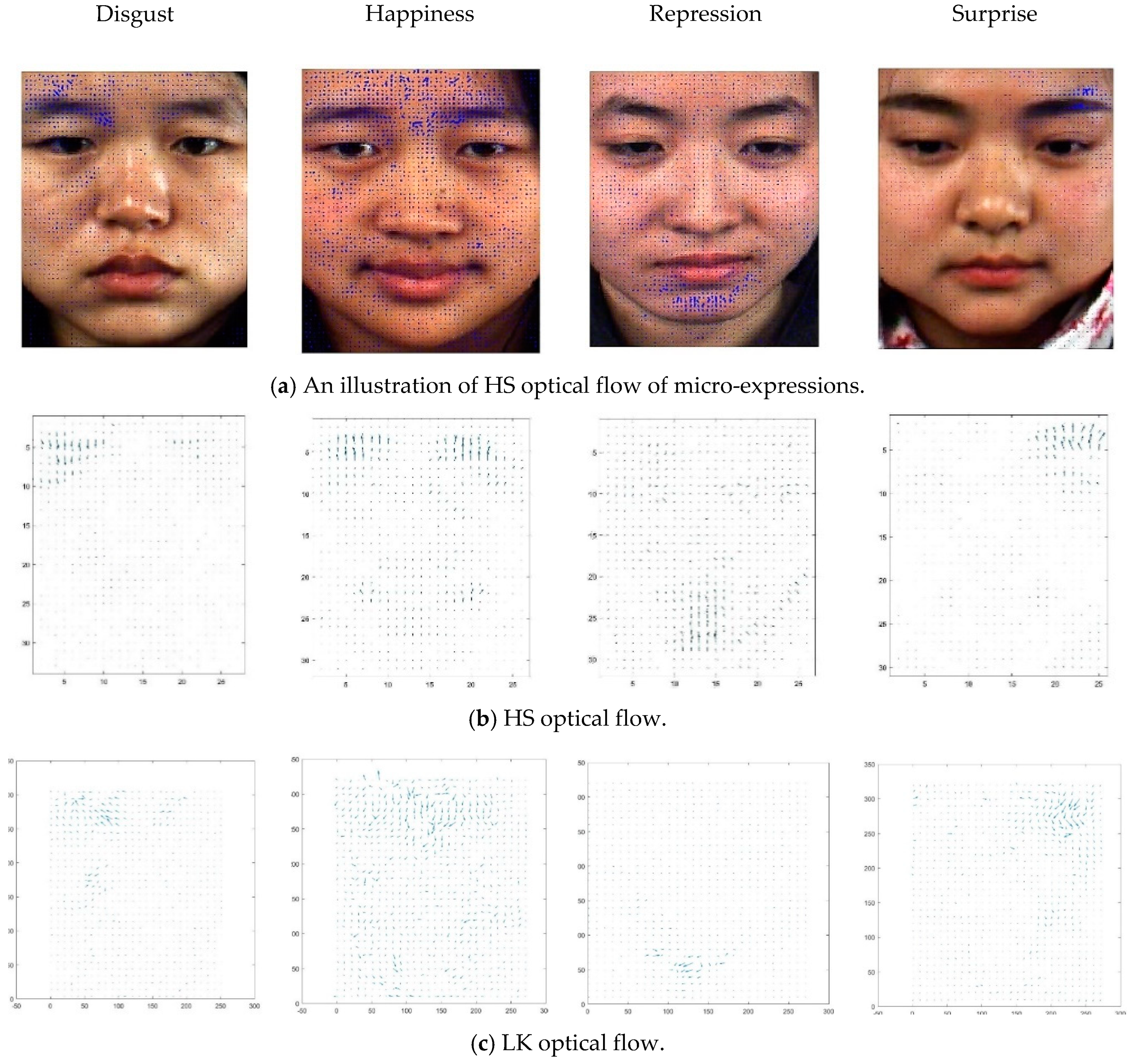
The dynamic regions calculated by optical flow in the CASME II database are shown in Figure 3. The result makes it clear that the active micro-expression patches are basically concentrated in the eyebrows, eyes, nasolabial groove and mouth. This experiment showed that the local motion characteristics suggested by Ekman [5]. For instance, arrows on the left corner of the mouth have an upward motion trend when a person is in an emotional state “Happiness” as shown in Figure 3, which indicates the optical flow can well track the changes of active patches. To obtain the accurate active location of active patches, in this paper we normalized micro-expression images to 240 × 280 and divided them into 12 × 14 patches. Then each piece was 20 × 20, and we calculated the optical flow for each active patch. In

Table 1. Emotion description in terms of facial action units and active patches.

Face Regions	AU(s)	Emotions
Eye + Eyebrow	1, 2, 4, 7	Disgust, Repression, Surprise
Nose	9	Disgust
Cheek	6	Happiness
Mouth	10, 12, 14, 15, 25	Disgust, Happiness, Surprise, Repression

, we summarize the relationship between the active patches in CASME II database and the AUs, whereas Figure 4 illustrates the locations of the AUs on the face.

In this paper, we extracted 106 active patches that were mainly distributed in the eyes, eyebrows, cheek, nose and mouth regions, as shown in Figure 4. These patches were obtained via an optical flow computation, which has more drastic movements, as indicated by the experimental section. They were also empirically selected (according to the AUs) while the micro-expression occured.

2.3. Feature Extraction

In the previous section, we used the optical flow to determine the facial active patches. We leveraged the optical flow features and the LBP-TOP descriptors to form a hybrid feature that indicates the motion and textural features needed for micro-expression recognition in the section. To identify the micro-expression, we needed to convert the optical flow into a set of corresponding features, therefore we divided the optical flow direction into 12 subspaces according to the size of the optical flow direction ((0, 30); (30, 60); (60, 90); (90, 120); (120, 150); (150, 180); (180, 210); (210, 240); (240, 270); (270, 300); (300, 330); (330, 360)). The frequency distribution of optical flow in all subspaces to generate an optical flow histogram is shown in Figure 5.

Figure 5 illustrates the directional histogram of “Happiness”. The X-coordinate was used for the 12 direction subspaces, while the Y-coordinate was for the corresponding proportion of the 12-feature dimensions. The extremely subtle optical flow does not cause muscle movement, so it was placed in the subspace of (0, 30). Other optical flows were placed in the corresponding subspaces according to their direction. As shown in Figure 5, the proportion of the first subspace (0, 30) was much higher than the others, which occured because most facial areas are hardly moved and were caused by the low-intensity micro-expressions. Only some specific regions such as the eyebrows, eyes, nose and mouth show significant changes. Nevertheless, the optical flow has defects that only consider the direction, so we use the LBP-TOP operator to supplement the textural features of micro-expressions.

To extract the dynamical texture features of the micro-expression sequences, Zhao et al. [10]. proposed the LBP-TOP operator, which separates the spatio-temporal regions into 3 orthogonal planes: XY, XT, and YT. The LBP values were then calculated from the center pixels in the three planes, which were later cascaded them into the feature vector.

If the video sequence has a low frame-rate and high-resolution, then the change of texture is more intense than the time change. Thus, we need to setup different radius parameters of space and time, as shown in Figure 6. The radius of the X, Y and T axis are represented by $R_X$, $R_Y$, $R_T$, while the number of pixels in the XY, XT, YT planes are characterized $P_{XY}$, $P_{XT}$, $P_{YT}$. The LBP-TOP histogram is now defined as:

$$H_{i,j}={\sum }_{x,y.t}I\left\{f_j\left(x,y,t\right)=i\right\}i=0,1,2,\cdots ,n_{j-1} j=0,1,2$$

(18)

where, j represents the numerical label assigned to the plane; j = 0 represents the XY plane, j = 1 represents the XT plane, and j = 2 represents the YT plane. The term $n_j$ is the number of binary modes generated by the LBP operator on the jth plane, where the feature extraction is carried out via an uniform mode operator: $LB{P}_{\left(8,R\right)}^{u2}$, for $n_j$ = 59. Since the XY plane contains textural information, the XT plane and YT plane contain motion information of the time domain, so the LBP-TOP histogram, formed by XY, XT and YT histograms, reveals the dynamic texture information in the space and time domain. Because there are only 12 dimensions of the optical flow histogram, the description of the micro-expression motion is too broad. The improvement initiated by the potential LBP-TOP operator was limited. Thus, a combination of optical flow and LBP-TOP features were considered to compensate for the algorithm’s own weaknesses to improve recognition performance.

In this paper, the LBP-TOP operator cascade histogram of three directions (XY, XT and YT) was used, and the feature dimension was 3 × 59 = 177. Moreover, the optical flow histogram had only 12 dimensions, so the description of motion was too broad and not detailed, and the improvement potential of LBP-TOP operator was limited. We considered combining optical flow histogram and LBP-TOP features to make up for their respective shortcomings, form a new feature, and further improve the recognition accuracy [32]. We used cascade histogram to combine optical flow features with LBP-TOP characteristics, as shown in Figure 7. The combined feature dimension is 177 + 12 = 189, of which the first 177 dimensions are the LBP-TOP feature and the last 12 dimensions are optical flow feature. The overall dimension changes of this feature are in the acceptable range, and the joint histogram retains the respective characteristics of the two algorithms without missing information.

2.4. NMP Extraction from the Active Patches

We began by separating each micro-expression image into 12 × 14 patches [33]. Then, we extracted the joint histograms that combines the optical flow with the LBP-TOP features in the active facial patches. Several active patches used for classification also affects speed and accuracy. There were up to 106 active patches with micro-expression that calculated by the proposed method. The dimension of a single image was up to 20,034 dimensions (i.e., $106\times \left(3\times 59+12\right)=\mathrm{20,034}$). Moreover, the classification accuracy was decreased if the feature dimension was too high. The motion amplitude of every micro-expression was very small. Using all the active patches for micro-expression recognition may add a lot of redundant information. Psychology research explains that micro-expressions are different from traditional expressions; only some special NMPs can recognize micro-expressions [9]. In this paper, a random forest feature selection (RFFS) method was used to choose the NMPs from 106 facial active patches for micro-expression recognition.

The random forest (RF) algorithm is a machine learning method, where the basic idea is to extract K-sample sets from the original input training sets. The extraction process is realized by a random resampling technique called bootstrapping [34]. Furthermore, we also need to ensure the size of each sub-sample set is the same as that of the original training set, as shown in Figure 8. Next, we set-up a K-decision tree model for the sample sets to get K kinds of classification results. Lastly, the classifier with the most votes is our result. RF algorithms can analyze and identify the interaction features quickly (i.e., learning speed is fast). The importance of its variables can be used as a tool for feature selection.

In this paper, to train the RF algorithm, we extract 106 active patches form each micro-expression and calculate the joint histogram integrated by the optical flow feature and LBP-TOP operator of each patch. Ultimately, they form the 106-feature histogram vectors as shown in Equation (19).

$$\{\begin{array}{c}\begin{array}{c}{v}_{eyebrow+eye}=\left[v_1,v_2,\cdots v_{40}\right]\\ v_{nose}=\left[v_{41},v_{42},\cdots v_{64}\right]\end{array}\\ v_{cheek}=\left[v_{65},v_{66},\cdots v_{82}\right]\\ v_{mouse}=\left[v_{83},v_{84},\cdots v_{106}\right]\end{array}$$

(19)

The feature input of an RF method is $\mathrm{V}=\left[v_{eyebrow + eye},v_{cheek},v_{nose},v_{mouse}\right]=\left[v_1,v_2,\cdots v_{106}\right]$, and the feature selection process is as follows:

Input: The training samples (N) and feature vectors (M) (where M = 1, 2, ⋯, 106)

Output: The F features with the most importance

Step 1: The Gini index is used to measure the segmentation effect of a feature in a decision tree by randomly sampling N and M;

Step 2: Repeating Step 2 to make K trees to constitute the forest;

Step 3: Calculating the classification error of the out-of-bag data of each tree: $\mathrm{error}OO{B}_1,\mathrm{error}OO{B}_2,\cdots ,\mathrm{error}OO{B}_k$;

Step 4: Randomly changing the value $v_j$ (where $v_j$ is the jth attribute of the feature vectors), and re-calculating the out-of-bag data: $\mathrm{error}OO{B}_1^j,\mathrm{error}OO{B}_2^j,\cdots ,\mathrm{error}OO{B}_k^j$;

Step 5: Calculating the importance of feature vector $v_j$: $Im{p}^{v_j}=\frac{{\sum }_{i=1}^K{\sum }_{j=1}^{M}errorOO{B}_i^j-{\sum }_{i=1}^{K}errorOO{B}_i}{K}$

Step 6: Repeating Step 5 to get the importance of all the features, then selecting the most indispensable features. Figure 8 shows the relationship between the number of features and the classification accuracy.

Figure 9 shows that the use of features from all 106 patches can classify every expression with a recognition rate of 62.03 percent or greater. Thus, the use of appearance-based features of a single active patch can discriminate between each expression efficiently and has a recognition rate of 50.9 percent. This implies that the use of the rest of the features from other patches contribute minimally towards the discriminative features. Thus, we see that the more patches are used, the larger the size of the feature vector. This increases the computational burden. Therefore, instead of using all the facial patches, we relied on some salient facial patches for expression recognition. This improved the computational complexity as well as the robustness of the features, which is especially true when a face is partially occluded. In our experiments, the recognition rate increased generally with the increasing number of active patches; it reached the highest level in the 60-th patch. Then the classification accuracy gradually declined as the unimportant features increase. This is mainly because the uncorrelated and redundant features reduce the performance of the classifier. As shown in

Table 2. Necessary morphological patches (NMPs) of micro-expression in the CASME II database.

Facial Regions	Emotion	Number of the NMPs	The Total
Eye + Eyebrow	Surprise, Disgust	1–18, 22–39	24
Nose	Disgust	49, 50, 53–64	14
Cheek	Happiness	66, 67, 69, 70, 74, 75, 77, 78	8
Mouth	Surprise, Repression, Happiness	85–88, 92–97, 101–104	14

, we summarized the NMPs numbers of the five areas (eyebrows, eyes, nose, cheeks and mouth) where micro-expressions are most intense and their corresponding emotional states.

2.5. Classifier Design

In this study, we used the support vector machine (SVM) as a classifier for micro-expression recognition [3]. However, micro-expression recognition is a multi-classification problem. There are two common methods to solve this problem: one-versus-rest (OVR) and one-versus-one (OVO). In this paper, we used OVO SVMs. The goal was to design an SVM between any two samples classes; thus, we needed to design k(k − 1)/2 SVMs. Next, when classifying an unknown sample, the sample used will determine the class with the largest number of votes. The advantage of this method is that it does not need to retrain all the SVMs, but only needs to retrain and add classifiers related to the samples. Additionally, we also needed to use a kernel function to map the sample from the original space to a higher-dimensional feature space, to ensure that the sample is linearly separable in this feature space. The kernel functions include a linear kernel, polynomial kernel, and Radial Basis Function (RBF). In this work, an RBF kernel, characterized by $\mathrm{k}\left(x_i,x_j\right)=\exp \left(-\frac{x_i-{x_j}^2}{2{\sigma }^2}\right)$ is used as our classifier.

3. Databases Processing and Experimental Settings

Micro-expression data acquisition is difficult, and it is difficult for non-professionals to identify micro-expressions too. Therefore, the collection and selection of micro-expression datasets is very important. There are two popular spontaneous micro-expression datasets to make experiment: the CASME II and SMIC databases [11,35]. This paper experimented on these two databases and describes the experimental setup and some details.

3.1. CASME II

The CASME II database [35] was published in 2014 as an upgraded version of the CASME database [36]. The time resolution of the new database changed from 60 fps to 200 fps, while the spatial resolution increased to a 280 × 340. The onset frame, the frame with the greatest variation (apex frame) and the offset frame of these micro-expression samples are coded. In addition, their facial motion units are marked and their emotional attributes are determined. These micro-expressions are grouped into two groups because of their different environmental configurations and different cameras used. Group A was taken by BenQ M31 camera at 200 fps and in natural light. Group B was shot by a Point Grey GRAS-03K2C camera at 200 fps. Group B was shot in a room with two LED lights. This dataset consists of five classes of emotions: happiness (32 samples), disgust (60 samples), surprise (25 samples), repression (27 samples) and tense (102 samples).

3.2. SMIC

The Spontaneous Micro-Expression Database (SMIC) was designed by the Zhao team at the Machine Vision Research Center of the University of Oulu, Finland [11]. The SMIC database included 164 micro-expression video clips from 16 participants (mean age 28, 6 women, 10 men, 8 Caucasians and 8 Asians). All the fragments are from HS data group, and there are 71 fragments from 8 participants of VIS and NIR data group. These micro-expressions were recorded in the interrogation room where threatening criminals were punished. Only a few emotional fragments containing high intensity were intercepted, and high intensity of emotional fluctuations prompted participants to suppress their facial expressions. Each micro-expression has a maximum total duration of 0.5 s and the longest video sequence contains 50 frames. There are three main emotion categories: positive (happiness; 51 samples), negative (sad, fear, and disgust; 70 samples), and surprise (43 samples).

3.3. CAS(ME)²

The Chinese Academy of Science Macro- and Micro-expression (CAS(ME)²) dataset [37] was established by the Chinese Academy of Science. In this dataset, 22 participants (13 females and 9 males) were asked to give response to nine chosen elicitation videos under two light-emitting diode (LED) lights. The dataset contains 300 macro-expressions and 57 micro-expressions, and also provides four different emotional labels: positive, negative, surprise and others. The expression samples in these dataset were selected from more than 600 elicited facial movements and were coded with the onset, apex, and offset frames, with AUs marked and emotions labeled [37]. In our experiments, all 357 video clips are used.

3.4. Experimental Settings

The micro-expression sequences, captured by a high-speed camera, are different from frame-to-frame. If the different frame numbers of each subject are used to extract and classify the micro-expressions, the recognition rate will degrade. Thus, we used the time interpolation model (TIM) to normalize all the frames of micro-expression sequences [38].

Table 3. Relationship between time interpolation model (TIM) length with time and accuracy.

TIM Length	no TIM	8	10	20	30	40
time (s)	87.8	16.7	22.1	49.6	77.2	104.9
accuracy	54.84%	57.15%	59.05%	57.80%	57.40%	56.93%

shows the relationship between the number of frames, the experimental time and accuracy. The frames of all samples were normalized to 10 (as in Table 3).

We used the facial landmark method in literature [27] to locate micro-expressions. The model is based on a mixtures of trees with a shared pool of parts; it models every facial landmark as a part and uses global mixtures to capture topological changes due to viewpoint. The experimental result shows that tree-structured models are surprisingly effective at capturing global elastic deformation, while being easy to optimize, unlike dense graph structures. We used this method to track all micro-expression sequences in three databases (CASME II, SMIC and CAS(ME)²). The experimental results are shown in

Table 4. The accuracy of landmark algorithm.

Parameter	CASME II	SMIC			CAS(ME)2
		HS	VIS	NIR
Sequence number	255	164	71	71	357
alignment number	249	160	71	70	348
accuracy rate	97.65%	97.56%	100%	98.59%	97.48%

.

In order to test the accuracy of the optical flow algorithm, we compared the average error and computational density of Horn-Schunck optical flow and Lucas-Kanade optical flow. The average error is the angle difference arcos $\left(1+V^{\prime }\times \mathrm{V}\right)$ between the calculated optical flow field $V^{\prime }=\left(v_1^{\prime },v_2^{\prime }\right)$ and the measured optical flow field $\mathrm{V}=\left(v_1,v_2\right)$. Computational density is the proportion of the pixels involved in the calculation. A larger computational density means that a more complete optical flow field can be provided. The calculation density is related to the average error. In the calculation, we chose a better optical flow algorithm based on these two calculation indexes.

From the results in

Table 5. Accuracy list of optical flow.

Database	Average Error/(%)		Computational Density/(%)
	Horn-Schunck	Lucas-Kanade	Horn-Schunck	Lucas-Kanade
CASME	13.88	11.74	100	92
SMIC	12.93	11.24	100	90
CAS(ME)2	14.23	11.98	100	93

, it can be seen that the classical Horn-Schunck and Lucas-Kanade optical flow algorithms are not suitable for dealing with large displacement, but they have good descriptive ability for small relative motion. This characteristic is very consistent with the muscle movement characteristics of micro-expressions.

In this paper, we used two cross-validation methods to evaluate the prediction performance of this model, which can alleviate the detrimental effects brought about by the over-fitting problem and can obtain as much effective information as possible from the limited data. The micro-expression dataset can be divided into three parts: the training set, the validation set and the test set. The training set is used to train the model, the verification set is used to configure the parameters, and the test set is the unknown data used to development the model, which is also used to evaluate the generalization ability of the algorithm. The leave one sample out cross validation (LOSOCV) method and the 10-Fold Cross Validation method were used to demonstrate the RF algorithm.

We used the SVM classifier to judge the recognition rate of NMPs. In the process of SVM classification and recognition, three important parameters need to be selected and adjusted. One is the selection of the kernel function. As shown in

Table 6. Recognition rate of different kernel functions on Chinese Academy of Science Macro- and Micro-expression (CASME II) and Spontaneous Micro-Expression (SMIC) databases (%).

Kernel Function	CASME II		SMIC		CAS(ME)2
	LOSOCV	10-Fold	LOSOCV	10-Fold	LOSOCV	10-Fold
SVM (polynomial)	59.53	61.09	57.28	58.04	59.87	62.20
SVM (linear)	58.05	60.76	55.68	57.39	59.05	61.52
SVM (RBF)	60.58	62.03	58.48	59.56	62.37	64.07

, in the experiment, we used all 106 valid regions to test and selected the kernel function and get the result with the highest recognition accuracy. The second is the penalty coefficient C, which is tolerance of errors. It can be used to compromise the minimization of training errors and the complexity of the model. The higher C shows that errors cannot be tolerated; it is easy to over-fit. The smaller C is, the easier it is to under-fit. The third is the gamma parameter, which is a parameter of RBF function when it is selected as kernel. The width of RBF will affect the range of action of each support vector corresponding to Gauss, thus affecting the generalization ability. In this paper, two cross-validation methods are used to predict the classification performance of machine learning model and the corresponding experimental results are given.

4. Results and Discussion

In this chapter, the NMPs definition of micro-expressions was proposed, and we also designed the corresponding experiments to verify their correctness and effectiveness.

4.1. Defined Active Patches and Feature Extraction

First, an automated learning-free facial landmark detection technique (proposed in [27]) was used to locate the facial region of each micro-expression sequence. Then the facial area was cropped according to a set of 68 landmarks. Ultimately, we normalized all the micro-expression images into 240 × 280-pixels and divided them into a set of 12 × 14 patches, each with 20 × 20 pixels, as shown in Figure 10, which also illustrates the location of the active patches and their associated emotional states.

The optical flow method was used to define the facial active patches of the micro-expressions, which the histograms were used as direction features to identify the micro-expression sequences. In this experiment, we analyzed the recognition rate of HS and LK optical flow algorithm on the CASME II database and chose the HS method with higher accuracy combined with LBP-TOP operators to form the ultimate micro-expression feature.

The recognition rate of optical flow features is low, as shown in Figure 11, and the proportion of erroneous decisions for each emotional category is high. There are two reasons for this problem: (1) the images in the database cannot (strictly) satisfy the assumption that the illumination remains unchanged, even if the appropriate experimental environment is set-up, thus, the brightness changes in the facial region are not complete eliminated; and (2) micro-expressions are subtle movements, which easily lead to over-smoothness and confuse some useful information.

To make-up for the deficiencies, LBP-TOP operators are calculated to cascade with optical flow features. An LBP-TOP operator has two important parameters: radius and neighborhood points. In this article, we write $\mathrm{LBP}-{\mathrm{TOP}}_{R_X,R_Y,R_T,P_{XY},P_{XT},P_{YT}}$ as $R_X,R_Y,R_T$; $P_{XY}=P_{XT}=P_{YT}=P$ for convenience.

Comparing the information in

Table 7. Recognition accuracies of different parameters (%).

${\mathit{R}}_{\mathit{X}},{\mathit{R}}_{\mathit{Y}},{\mathit{R}}_{\mathit{T}},\mathbf{P}$	Accuracy	${\mathit{R}}_{\mathit{X}},{\mathit{R}}_{\mathit{Y}},{\mathit{R}}_{\mathit{T}},\mathbf{P}$	Accuracy	${\mathit{R}}_{\mathit{X}},{\mathit{R}}_{\mathit{Y}},{\mathit{R}}_{\mathit{T}},\mathbf{P}$	Accuracy
111, 4	46.20	111, 8	47.85	111, 16	47.02
331, 4	49.50	331, 8	50.33	331, 16	47.85
333, 4	45.37	333, 8	47.03	333, 16	47.68

, the recognition rate of $R_X=R_Y=3,R_T=1$; $P_{XY}=P_{XT}=P_{YT}=8$ is the highest. This is due to the high resolution of the micro-expression images and short inter-frame space. Thus, we need a larger spatial domain. $R_X$ and $R_Y$, a smaller time domain $R_T$ that embodies local textural properties and spatial-temporal motion information. Moreover, the neighboring points will also affect the accuracy of recognition. If P is too small, the feature dimensions are insufficient, lack of sufficient information; if P is too large, it will produce high-dimensional features that will confuse the distinction between classes and significantly increase the number of calculations.

4.2. NMPs Defined and Result Comparison

In the experiments discussed in Section 4.1, we extracted 106 active facial patches to represent the muscle motion profile of micro-expressions. We then extracted the features based on the combination of optical flow features and LBP-TOP operators of these patches. If all active patches are used for micro-expression recognition, this will not only cause high-dimension features but will also fail to show the necessary emotional state of micro-expressions. So, we used the RFFS method to measure the importance of these active patches and select the NMPs with the most discriminant ability to recognize micro-expressions. We conducted experiments in the facial area, the active patches and the NMPs. The results are shown in

Table 8. Recognition rate in different regions of micro-expressions in the CASME II database (%).

Method	Optical Flow		LBP-TOP		Fusion Feature
	LOSOCV	10-Fold	LOSOCV	10-Fold	LOSOCV	10-Fold
whole face	39.56	41.08	50.33	51.83	58.12	59.46
Activepatch (106)	41.29	43.00	53.67	54.24	60.58	62.03
NMPs	45.73	46.89	57.09	58.90	72.08	73.51

,

Table 9. Recognition rate in different regions of micro-expressions in the SMIC database (%).

Method	Optical Flow		LBP-TOP		Fusion Feature
	LOSOCV	10-Fold	LOSOCV	10-Fold	LOSOCV	10-Fold
whole face	37.14	38.24	48.97	49.33	55.01	57.00
Activepatch (106)	40.06	42.05	52.00	53.41	58.48	59.56
NMPs	43.98	44.78	55.82	56.90	69.37	70.02

and

Table 10. Recognition rate in different regions of micro-expressions in the CAS(ME)² database (%).

Method	Optical Flow		LBP-TOP		Fusion Feature
	LOSOCV	10-Fold	LOSOCV	10-Fold	LOSOCV	10-Fold
whole face	38.96	40.62	50.97	52.70	58.67	61.00
Activepatch (106)	42.59	43.97	53.93	56.84	64.09	65.56
NMPs	45.02	47.08	58.14	58.04	72.96	74.73

.

As a feature selection algorithm, RF can evaluate the importance of each patch on the classification problem. This paper also used other feature selection methods to select the NMPs for micro-expression recognition and to obtain the corresponding accuracy. The experimental results are shown in

Table 11. Accuracy rate and NMPs numbers of different feature selection algorithms.

NMP Number	Pearson Coefficients	Mutual Information	Lasso Model	RF
eye + eyebrow	22	20	27	24
nose	4	3	15	10
cheek	0	0	10	12
mouth	13	10	15	14
Recognition rate	57.37%	55.09%	65.10%	73.51%

.

By comparing the data in the table, several NMPs in the eyes, eyebrows and mouth regions (selected by each algorithm) are essentially equivalent, while the NMPs in the cheek and nose regions are different. This is because the muscle movement of micro-expressions are mainly concentrated in the eyes, eyebrows and mouth regions. There are few AUs for the cheek and nose regions, while the micro-expressions are restrained movements, which are very subtle and easily overlooked. In some regions, the correlation of motion is very small, so the Pearson Coefficient is insensitive and misleading. Mutual information as a feature selection method is not convenient. It is not a measurement method, nor can it be normalized, and the results on different data sets cannot be compared. The Lasso model is also very unstable, when the data changes slightly, the model changes drastically. The proposed method is robust and useful, and the experimental results show that the NMPs selected by this method are basically in-line with the most representative facial muscle motion patches developed by psychologists.

This method can also reduce the dimensionality of features. Compared with other traditional methods, our proposed method can select some features with strong descriptions and improved discrimination ability.

Table 12. Comparison of recognition accuracies between different feature dimension methods (%).

Method	Recognition Rate
	LOSOCV	10-Fold
fusion feature algorithm + PCA	64.23	65.81
fusion feature algorithm + LDA	65.15	66.09
the proposed method	72.08	73.51

shows the experimental results of the comparison between our method and the traditional dimensional reduction methods used on the CASME II database.

The traditional feature reduction method only maps hybrid features, extracted from active patches, from the high-dimensional space to a new low-dimensional space. However, because the motion amplitudes of micro-expressions are very small, the traditional methods that don’t consider target variables in the process of dimensionality reduction are likely to remove features with key motion information. This will affect the accuracy of the classifier. In this paper, the RF algorithm was used to screen out the NMPs for micro-expression recognition. This algorithm is designed and implemented according to the experimental purpose of the article. The NMPs that have the greatest likelihood for micro-expressions were also highly-targeted and accurate. Thus, we needed to evaluate the importance of each active patch to select the most representative necessary areas. In addition, this algorithm can eliminate some irrelevant and redundant features to reduce the feature dimensions, improve the model accuracy and reduce the running time.

We compared the accuracy between the proposed method and the other micro-expression recognition algorithms [39,40,41,42,43,44,45,46,47,48,49,50]. The final results are shown in

Table 13. Micro-expression recognition rates (%) in the CASME II Database.

Method	Task	Recognition Rate
TICS [39]	happiness, surprise, disgust, repression, others	61.76
CUDA based DCNN [40]	happiness, surprise, disgust, repression, others	64.90
HIGO-TOP [42]	happiness, surprise, disgust, repression, others	55.87
HOG-TOP [42]	happiness, surprise, disgust, repression, others	57.49
DTSCNN [44]	happiness, surprise, disgust, repression, others	66.67
CNN-Net [45]	happiness, surprise, disgust, repression, others	75.57
RoI-Selective (LBP-TOP) [46]	happiness, surprise, disgust, repression, others	46.00
Hierarchical STLBP-IP + KGSL [47]	happiness, surprise, disgust, repression, others	63.97
FMBH [48]	happiness, surprise, disgust, repression, others	69.11
Sparse MDMO [49]	happiness, surprise, disgust, repression, others	66.95
Apex-frame (Bi-WOOF) [50]	happiness, surprise, disgust, repression, others	62.55
The proposed method	happiness, surprise, disgust, repression, others	73.51

and

Table 14. Micro-expression recognition rates (%) in the SMIC Database.

Method	Recognition Rate
CNN + SFS [41]	53.60
HIGO-TOP [42]	57.93
HGO-TOP [42]	59.15
FDM [43]	54.88
NMFL [43]	62.33
RoI-Selective (LBP-TOP) [46]	54.00
Hierarchical STLBP-IP + KGSL [47]	60.37
FMBH [48]	71.95
Sparse MDMO [49]	70.51
Apex-frame (Bi-WOOF) [50]	68.29
The proposed method	70.02

. The tables show that our algorithm has better recognition performance on the two databases.

As shown in Table 12, both of the methods produce different accuracy in the CASME II database, while the proposed method in this paper and CNN-Net method take a better recognition rate. Although the other methods find some useful features for micro-expression, they sometimes fail to consider the psychological mechanisms involved to emotional state of micro-expression, especially on the NMPs. The CNN-Net algorithm [45] achieves higher accuracy from experimental results, but it has a fatal flaw: the uninterpretability of deep neural networks. However, the research of micro-expression recognition is still very immature and its mechanism is very unstable. Most micro-expression researchers focus on how to better understand the principle of micro-expression generation and the deeper emotional state behind it by means of machine learning. The uninterpretability of deep learning is inconsistent with the purpose of these studies, so in this paper we did not choose deep network as a learning tool for micro-expression recognition.

5. Conclusions

The main contribution of this paper is the analysis and determination of the NMPs for micro-expression recognition. Previously, only psychologists suggested that micro-expressions have specific NMPs and have the crucial ability to describe micro-expressions. This paper first applied the psychological concept to the field of computer recognition; it used related techniques to extract these important (feature) patches. We compared the optical flow between the on-set frame and the apex frame in this study. We then defined the regions that are full of muscle movements as potential facial active patches of the micro-expression sequences. The optical flow direction histograms and the LBP-TOP operators in these patches were cascaded into the joint features of micro-expressions. The random forest feature selection technique was used to select NMPs with discriminant ability. Finally, we tested the effectiveness of the proposed method via two famous spontaneous micro-expression databases. The experiments showed that NMPs can describe the muscle movement of micro-expressions better than using the whole facial region for recognition. It also eliminates several redundant features, reducing the feature dimension and improving the recognition accuracy.

In this paper, the NMPs of micro-expressions were automatically extracted. Some related psychological research shows that every emotion has its own specific necessary patches. Thus, in future studies, we will focus on analyzing the specific NMPs of each emotion and apply these patterns to automatic micro-expression recognition.