A Multi-Objective Programming Approach to Design Feeder Bus Route for High-Speed Rail Stations

Abstract

The quality of route design can greatly affect the operational efficiency of feeder bus service for high-speed rail stations. A bi-objective optimization formulation is established to consider the trade-off between two conflicting optimization objectives, namely maximizing the travel demand that can be served and minimizing the feeder bus route length. The Pareto optimal solutions of the discrete mathematical formulation are generated by the exact ε-constraint method. We test the proposed approach with a numerical example on an actual size scale. The results indicate that the computational efficiency of the solution approach is encouraging, and a series of route design plans and location stop plans are generated simultaneously in a short time. A numerical example also shows that as the passengers’ maximum acceptable walking distance increases, more travel demand can be served when the route length does not change much. Benefits brought by increasing feeder bus route length are analyzed and the robustness of obtained solutions is verified. The comparison of our approach and an existing approach is also presented to demonstrate that our approach can generate better solutions.

1. Introduction

In recent years, as the mileage of high-speed railway and high-speed rail stations increase rapidly, the travel demand for high-speed railway in China has also increased. This leads to a lot of passengers bound for or leaving high-speed rail stations. Many high-speed rail stations are in the suburbs, far away from the urban central areas. Considering the considerable expense, taking a taxi is usually not chosen by many passengers. Driving may result in a parking problem at high-speed rail stations. While the feeder bus system can expand the rail transport catchment area beyond walking distance, particularly for passengers who do not have vehicles or cannot afford the parking expense [1]. Moreover, the trips bound for or leaving high-speed rail station access present a one-to-many or many-to-one traveling character. Therefore, the high-speed rail stations need the feeder bus to concentrate and diffuse many travelers. The feeder bus system is the only public alternative except for private modes (driving and taxi) for high-speed rail stations, especially when the stations are not connected to the subway system [2].

In the planning stage of the feeder bus service, decision makers usually need to consider several critical problems, e.g., how to choose the locations of stops and how to design efficient feeder bus routes. Proper stop locations and high-quality feeder bus routes can lead to a decrease of passengers’ travel cost and make the feeder bus system serve more travel demand. Realizing the above critical problems, our study is concerned about route design as well as the stop location of the feeder bus service for high-speed rail stations.

Designing feeder bus routes for high-speed rail stations differs from designing a traditional bus route. Since passengers may transfer frequently and their route plans may be complex, traditional bus route design problems must take into account passengers’ route choice behaviors, which results in a very complex problem. The feeder bus system for high-speed rail stations mainly serves the passengers bound for or leaving high-speed rail stations, which means that the distribution of travel demand is mainly many-to-one or one-to-many. Therefore, designing feeder bus routes for high-speed rail stations is more independent and easier.

Considering that many high-speed rail stations are in the outskirts, the feeder bus service should aim at enhancing high-speed rail stations’ accessibility and attracting more passengers to choose high-speed railways for their intercity travel [3]. To enhance high-speed rail stations’ accessibility, we hope to serve more travel demand and reduce the feeder bus route length. The feeder bus route length can influence passengers’ in-vehicle travel time. Therefore, passengers often wish that the feeder bus routes were shorter. Furthermore, if the feeder bus can serve more travel demand, the attraction of high-speed railways can also be enhanced. According to Fan [4], it is usually impossible to serve all travel demand because of limited public transport supplies. Hence, the travel demand that can be served is supposed to be as large as possible. These two objectives may be conflicting. Serving more travel demand usually indicates that there may be more detours and bus stops along the feeder bus route. However, the travel demand that can be served often decreases as route length reduces, because some stops may be removed or may not be located within passengers’ acceptable walking distance. A crucial trade-off exists between the two-optimization objectives. It is important for decision makers to find this trade-off.

Our work aims to propose a multi-objective approach to design the route of the feeder bus service for high-speed rail stations and decide the stop locations simultaneously. Literature related to the design of feeder bus routes for high-speed rail stations and works on the problems closely related to our research are reviewed in Section 2. In Section 3, we put forward a bi-objective mathematical model to obtain stop locations and a feeder bus route for a high-speed rail station. Then, Section 4 shows how the proposed problem is solved by an exact ε-constraint method. In Section 5, a numerical example of actual scale is shown to test our approach. In Section 6, some conclusions are shown.

2. Literature Review

Stop location is significant to the bus routing problem [5]. Obviously, the bus stop is the entrance of a bus system [6]. The stop location will affect whether passengers would choose to travel by public transport mode, especially for the feeder bus service for high-speed rail stations. Given that passengers may carry luggage or catch a train, a long walking distance between stops and demand points may reduce passengers’ willingness to choose this feeder bus service. Moreover, the stop location can affect the feeder bus route length as well as passengers’ in-vehicle time, thus the choice of passengers can also be influenced. Therefore, the travel demand for the feeder bus service for high-speed rail stations is certainly connected with the stop location.

An examination of existing research on the feeder bus system, however, suggests that the stop location is often omitted in the literature [7,8,9,10]. In their works, the stop location is neglected and the travel demand for the feeder bus service is related to route links, which is based on some assumptions, i.e., buses can pick up or drop off passengers anywhere along the bus route, or travel demand is homogeneously distributed along route links or in traffic zones. However, these assumptions may be invalid in China. Because buses can only pick up or drop off passengers at bus stops instead of in front of buildings [11]. Moreover, Teng et al. [3] propose an approach to design feeder bus routes for high-speed rail stations. They assume that if a traffic zone is passed by the feeder bus route, the feeder bus system can serve this traffic zone. Therefore, the stop location is also not considered. This means that passengers cannot be served when they are in traffic zones which are not passed, even if they are near the feeder bus lines. Lin and Wong [12] present a formulation to generate feeder bus routes and the stop location is not taken into account based on the hypothesis that stop spacing is generally not longer than walking distance in dense urban areas. Whereas, this assumption may be invalid for our problem, given that feeder bus routes for high-speed rail stations may pass through outskirts where the travel demand density is sparse. The stop spacing usually exceeds a reasonable walking distance in the suburbs.

In other previous studies, the number and locations of bus stops are given as inputs, and bus stops are demand points [13,14,15,16,17,18,19,20,21]. This assumption is reasonable when feeder bus routes are designed considering existing stops or the planner’ hope to adjust the existing feeder bus routes. However, it may not be reasonable if planners wish to make new plans from scratch or plans completely different from existing ones [22].

Recently, several approaches have been developed to decide both the stop location and bus route [23,24]. However, these approaches decide the stop location and bus route successively. Sequential methods solve the stop location problem first, then stop location is an input of route design. Based on its definition, sequential methods may generate sub-optimal plans. Limited scholars have attempted to solve the two problems simultaneously. An integrated routing and stop location problem is solved by Perugia et al. [22]. They establish a model considering bus stop location and routing while the number of stops is an input. As mentioned in the last paragraph, this assumption may be unreasonable when decision makers wish to make new plans. Therefore, the number of stops will be determined in our work. Xiong et al. [25] establish a model to design the route of community shuttle. A stop location algorithm is integrated in this model. They assume that for demand points, the nearest points on the route are stops. This assumption means that some necessary consideration such as stop spacing may be violated, which may be unreasonable. The most similar to our formulation are by Schittekat et al. [26] and Chen et al. [27]. Schittekat et al. [26] establish a programming formulation for school bus routes design problem with bus stop selections. The stops to be visited, the situation of matching students to stops and school bus routes can be obtained simultaneously by solving the model. The difference between the work of Schittekat and ours is that we propose a multi-objective approach, which can make us analyse the trade-off between operator’s cost and the travel demand that can be served. Considering the number of bus stops as an input, Chen et al. [27] discuss a suburban bus route design problem. They regard the many-to-one bus travel access to the airport as a discrete location-routing problem. Our problem can also be formulated as a discrete location-routing problem. In order to maximize the travel demand that can be served, locations of demand points and travel demand are also considered in our model, which is ignored by them.

In fact, our problem is also similar to some routing and scheduling problems in the domain of transportation, such as cash transportation vehicle routing and scheduling problem [28,29], first and last mile delivery problem [30,31,32], waste collection routing problem [33,34,35] and dial-a-ride problem [36,37]. Considering the locations of customers and some specific constraints (e.g., time windows and vehicle capacity), the solution approaches to these problems cannot be applied to our problem directly.

Previous studies on feeder bus routes design and related problems are summarized in

Table 1. Literature review.

Publication	Objective	Decision Variables	Travel Demand Pattern	Optimization Method for Bus Stop and Route
Chien and Yang. 2000	Minimize the summation of supplier cost and user cost	Bus route	Based on route links	-
Jerby and Ceder. 2006; Xiong et al. 2014; Zhu et al. 2017	Maximize the demand potential of the route links	Bus route	Based on route links	-
Teng et al. 2013	Maximize the population served by equivalent straight line of bus route	Bus route	Based on traffic zones	-
Lin and Wong. 2014	Maximize service coverage, minimize the maximum bus route travel time, minimize bus route length	Bus route	Based on demand nodes	-
Shrivastava and Dhingra. 2001; Song and Liu. 2011	Minimize bus route length	Bus route	Based on demand nodes (bus stops)	-
Kuan et al. 2004, 2006; Shrivastava and O’ Mahony. 2006, 2009	Minimize the sum of operator and user costs	Bus route and frequency	Based on demand nodes (bus stops)	-
Sun et al. 2011	Minimize the sum of operator, user costs and the opposite number of bus passengers	Bus route, timetable and choice behavior of passengers	Based on demand nodes (bus stops)	-
Szeto and Wu. 2011	Minimize the sum of the number of transfers and total passengers’ travel time	Bus route and frequency	Based on demand nodes (bus stops)	-
Liu et al. 2015	Minimize passengers’ travel time, maximize transport efficiency	Bus route	Based on demand nodes (bus stops)	-
Li and Chen. 2016	Minimize bus route length and passengers’ travel cost	Bus stop location and route	Based on demand nodes	successive
Leksakul et al. 2017	Minimize the sum of the distance between the bus stop and the passengers’ addresses, minimize route length	Bus stop location and route	Based on demand nodes	Successive
Perugia et al. 2011	Minimize the total cost of bus service, minimize the total extra-time	Bus stop location and route	Based on demand nodes (bus stops)	Simultaneous
Xiong et al. 2013	Minimize the sum of user cost and supplier cost	Bus stop location, route and headway	Based on demand nodes	Simultaneous
Schittekat et al. 2013	Minimize the total distance travelled by buses	Bus stop location and route	Based on demand nodes	Simultaneous
Chen et al. 2017	Minimize the total vehicular travel time	Bus stop location and route	neglected	Simultaneous
Yan et al. 2012, 2014	Minimize the carrier’s operating cost	Vehicle route	Based on demand nodes	-
Bányai. 2018	Minimize the energy use	Assignment of open tasks to delivery service provider, delivery route, scheduling of pickup and delivery operations	Based on pickup points and destinations	-
Bányai et al. 2018	Minimize the costs of the whole delivery process	Assignment of open tasks to scheduled routes, assignment of picked up packages to delivery routes or hubs, scheduling of pickup operations	Based on pickup points and destinations	-
Zhou et al. 2018	Minimize the sum of routing, connection and handling costs	Vehicle route	Based on demand nodes	-
Ramos et al. 2018	Minimize transportation cost	Vehicle route	Based on demand nodes	-
Tirkolaee et al. 2018	Minimize usage cost of vehicles and traversing cost	Vehicle route and optimal number of vehicles	Based on edges	-
Bányai et al. 2019	Minimize energy use of collection process	Assignment of households to routes of garbage trucks and scheduling of garbage trucks	Based on demand nodes	-
Riedler and Raidl. 2018	Maximize the number of served requests	Vehicle route, beginning-of-service time of vehicle, load of vehicle and ride time of request	Based on pick-up locations and drop-off locations	-
Tellez et al. 2018	Minimize the total transportation cost	Vehicle route, location for vehicle to be reconfigured, load of vehicle and service time of vehicle at node	Based on pickup locations and delivery locations	-

. In summary, to our knowledge, few studies have studied how to design feeder bus routes and determine stop locations simultaneously. The stop location and route design are closely related, and it is significant to consider the two aspects simultaneously. Therefore, in this study, the route design and stop location of feeder bus service for high-speed rail stations will be considered in an integral way and the number of stops will be determined simultaneously.

3. Problem Formulation

3.1. Problem Description and Assumptions

A description of the problem to be solved is first given below. There is a high-speed rail station on the outskirts of a city and far away from urban central areas of this city. Some demand points (e.g., residential areas, transit hubs/stations) are in the same city. Travel demand for the feeder bus service is given. There are also some candidate stops in this city and some of them will be selected as feeder bus stops. The locations of demand points and candidate stops are given. All distances are known, including the distances between candidate stops and between demand points and candidate stops. Passengers can only get on buses and get off at the stops. The goal is to determine the stop location and which demand points can be served by each stop. If a candidate stop is chosen as a stop, demand points within the maximum acceptable walking distance from this candidate stop can be served. Moreover, the shortest feeder bus route visiting these stops is designed. We hope to maximize the travel demand that can be served and minimize the route length of the feeder bus service for the high-speed rail stations.

As shown in Figure 1, two feeder bus routes connect a high-speed rail station with some demand points. In general, the feeder bus route starts from a transfer stop near the high-speed rail station. Circles represent the stops chosen from the candidate stops and arrowed solid lines represent the feeder bus route. Triangles represent the candidate stops, which are not chosen to be feeder bus stops. Candidate stops can be identified by expert judgment or selected from places with high travel demand based on the vehicle GPS data [38]. Generally located near the high-speed rail station, the transfer stop is marked as a square. At this stop, passengers can transfer between the high-speed railway and feeder bus service. We use gray circles to represent the demand points. The match situation between the demand points and the stops is shown by dash lines.

3.2. Mathematical Formulation

The sets, parameters, and decision variables are defined in

Table 2. List of notations.

Sets
D	set of demand points, $i,j\in D$
H	set of candidate stops, $k,l\in H$
Parameters
dkl	distance between candidate stops k and l
${\overline{d}}_k$	straight-line distance between the transfer stop and candidate stops k
qi	travel demand of demand point i
lmax	the maximum length of feeder route
lmin	the minimum length of feeder route
smax	the maximum stop spacing
smin	the minimum stop spacing
c	the maximum nonlinear factor
Dmax	the maximum acceptable walking distance of passengers
aik	binary assistant parameter, (1 if distance between demand point i and candidate stop k does not exceed Dmax and 0 otherwise)
Decision variables
xk	0-1 decision variable, equals to 1 if candidate stop k is chosen as a stop, and 0 otherwise
vi	0-1 variable, equals to 1 if demand point i can be served, and 0 otherwise
yik	binary variable (1 if demand point i can be served by candidate stop k and 0 otherwise)
zkl	binary variable (1 if candidate stop k and l are adjacent stops and 0 otherwise)
uk	nonnegative integer assistant variable to eliminate sub-tour

, before we present the mathematical formulation.

The mathematical formulation is as below.

$$\max C_1={\displaystyle \sum _{i\in D}{v}_i{q}_i},$$

(1)

$$\min C_2={\displaystyle \sum _{k\in H}{\displaystyle \sum _{l\in H,l\ne 1}{z}_{kl}{d}_{kl}}},$$

(2)

subject to

$$l_{\min }\le {\displaystyle \sum _{k\in H}{\displaystyle \sum _{l\in H,l\ne 1}{z}_{kl}{d}_{kl}}}\le l_{\max },$$

(3)

$$\begin{array}{cc}{z}_{kl}{s}_{\min }\le z_{kl}{d}_{kl}\le z_{kl}{s}_{\max },& \forall k,l\in H,l\ne 1,\end{array}$$

(4)

$${\displaystyle \sum _{k\in H}{\displaystyle \sum _{l\in H,l\ne 1}{z}_{kl}{d}_{kl}}}\le c{\displaystyle \sum _{k\in H}{z}_{k1}{\overline{d}}_k},$$

(5)

$$\begin{array}{cc}{x}_k\cdot a_{ik}=y_{ik},& \forall i\in D,k\in H,\end{array}$$

(6)

$$\begin{array}{cc}{\displaystyle \sum _{i\in D}{y}_{ik}}\ge x_k,& \forall k\in H,k\ne 1,\end{array}$$

(7)

$$\begin{array}{cc}{\displaystyle \sum _{l\in H,l\ne k}{z}_{kl}}={\displaystyle \sum _{l\in H,l\ne k}{z}_{lk}}=x_k,& \forall k\in H,\end{array}$$

(8)

x₁ = 1,

(9)

$$\begin{array}{cc}{u}_k-u_l+\left|H\right|z_{kl}\le \left|H\right|-1,& \forall k,l\in H,l\ne 1,l\ne k,\end{array}$$

(10)

$$\begin{array}{cc}{z}_{kk}=0,& \forall k\in H,\end{array}$$

(11)

$$\begin{array}{cc}{v}_i\le {\displaystyle \sum _{k\in H}{y}_{ik}},& \forall i\in D,\end{array}$$

(12)

$$\begin{array}{cc}{v}_i\ge y_{ik},& \forall i\in D,k\in H,\end{array}$$

(13)

$$\begin{array}{cc}{v}_i,x_k,y_{ik},z_{kl}\in \left\{0,1\right\},& \forall k,l\in H,i\in D,\end{array}$$

(14)

$$\begin{array}{cc}{u}_k\ge 0,& \forall k\in H,\end{array}$$

(15)

Objective (1) maximizes the travel demand that can be served by the feeder bus system. Objective (2) attempts to minimize the route length. This work applies constraint (3) to limit the upper-bound and lower-bound lengths of the feeder bus route. Constraint (4) depicts the minimum and maximum stop spacing. Constraint (5) underscores that the feeder bus route whose nonlinear factor in excess of an upper limit c is forbidden. Constraint (6) specifies that if a candidate stop is chosen as a stop, all demand points lying within the maximum acceptable walking distance away from it can be served. Otherwise, demand points cannot be served by this candidate stop. Constraint (7) ensures that if a candidate stop is chosen as a stop, at least one-demand points will be served by it. Using constraint (8), we calculate the degrees of stop vertices and ensure flow conservation at these vertices. Constraint (9) indicates that the first candidate stop, i.e., the transfer stop, must be selected as a stop. The sub-tour is eliminated by constraint (10). Constraint (11) ensures that each candidate stop cannot be visited twice by the feeder bus route. Constraints (12) and (13) guarantee v_i = 0 if no candidate stop can serve demand point i. Otherwise, v_i is equal to 1. Constraints (14) and (15) define the domains of the decision variables.

4. Solution Method

This paper studied a bi-objective optimization problem. One of the classical methods to solve multi-objective optimization problems is to allocate an importance weight to each optimization objective and convert the multi-objective problem into a single-objective one. However, decision makers often have difficulty in assigning the importance weights properly in reality. Hence, we are interested in providing the Pareto optimal front for decision makers. The Pareto optimal front is a set of Pareto optimal solutions. A Pareto optimal solution is one, which is not worse than any other solutions considering all objectives [39]. Moreover, a Pareto optimal solution is better than any solution in at least one objective. Each Pareto optimal solution represents a scheme of stop location and route design. Based on the above, this section presents an exact ε-constraint method proposed by Berube et al. [40] to find the Pareto optimal front.

Using the exact ε-constraint method, we select an objective as the main objective and optimized, while adding other objectives as constraints to the feasible solution space. We believe that in order to attract more passengers to choose the high-speed railway for intercity travel, it is more important to provide the feeder bus service for more passengers than to reduce in-vehicle time of passengers. Thus, for our problem, objective C₁ is chosen as the main objective and objective C₂ is added as a constraint, which is a single-objective optimization sub-problem as follows.

max C₁

subject to

(3)–(15)

$$C_2\le \epsilon ,$$

(16)

The pseudo code of the exact ε-constraint method is as follows:

Input: stop location and route design instance of feeder bus system for high-speed rail stations

Output:ParetoSet: the Pareto optimal front

1: $ParetoSet=\varnothing$

2: Solve $C_2^{\ast }=\left\{\min C_2:\left(3\right)–\left(15\right)\right\}$

3: Solve $C_1^{\ast }=\left\{\max C_1:\left(3\right)–\left(15\right)\right\}$

4: Solve $C_1^{\min }=\left\{\max C_1:\left(3\right)–\left(15\right),C_2\le C_2^{\ast }\right\}$

5: Solve $C_2^{\max }=\left\{\min C_2:\left(3\right)–\left(15\right),C_1\ge C_1^{\ast }\right\}$

6: $ParetoSet=ParetoSet\cup \left\{\left(C_1^{\ast },C_2^{\max }\right),\left(C_1^{\min },C_2^{\ast }\right)\right\}$

7: Set $\epsilon =C_2^{\max }-\Delta$

8: while $\epsilon >C_2^{\ast }$ do

9: Solve $C_1^{\epsilon }=\left\{\max C_1:\left(3\right)-\left(15\right),C_2\le \epsilon \right\}$

10: $ParetoSet=ParetoSet\cup \left(C_1^{\epsilon },C_2^{\epsilon }\right)$

11: Set $\epsilon =C_2^{\epsilon }-\Delta$

12: Remove dominated points from ParetoSet.

By changing the value of the right-hand side ε of the constraint (16) and solving a set of single-objective optimization sub-problems, the Pareto optimal front will be obtained. As mentioned above, the Pareto optimal front is first initialized as empty. Then, the optimal feeder bus route with the minimum route length is determined. Similarly, the optimal plan of the stop location that maximizes the travel demand that can be served is obtained. In Step 4, an extreme point of the Pareto optimal front is obtained by maximizing the travel demand that can be served and considering constraints (3)–(15) and $C_2\le C_2^{\ast }$. Similarly, Step 5 determines the other extreme point of the Pareto optimal front by minimizing the route length considering constraints (3)–(15) and $C_1\ge C_1^{\ast }$. $C_1^{\ast }$ and $C_2^{\ast }$ represent the maximum value of objective C₁ and the minimum value of objective C₂, respectively. Then ε is set as the difference between $C_2^{\max }$ and Δ, where Δ is a constant value and set to 1 in this article. We can obtain a Pareto optimal solution by maximizing the travel demand that can be served and considering constraints (3)–(15) and $C_2\le \epsilon$ in Step 9. The parametric variation of ε is implemented in Step 11. Dominated points in the Pareto optimal front are removed in Step 12 using the fast non-dominated sorting procedure. Readers can refer to Deb et al. [41] for more details on the fast non-dominated sorting procedure. Note that all single-objective optimization sub-problems above are solved by the ILOG CPLEX solver.

5. Numerical Example

In this section, we will present the numerical results obtained by our method. We use a numerical example on an actual size scale to demonstrate the computational efficiency of the solution method. Furthermore, the effect of the maximal acceptable walking distance of passengers on the Pareto optimal solutions is discussed in the numerical example. Benefits brought by increasing the feeder bus route length are also analyzed. Then, we verify the robustness of the Pareto optimal front. Finally, our approach is compared with an existing approach and the advantages of our approach are verified.

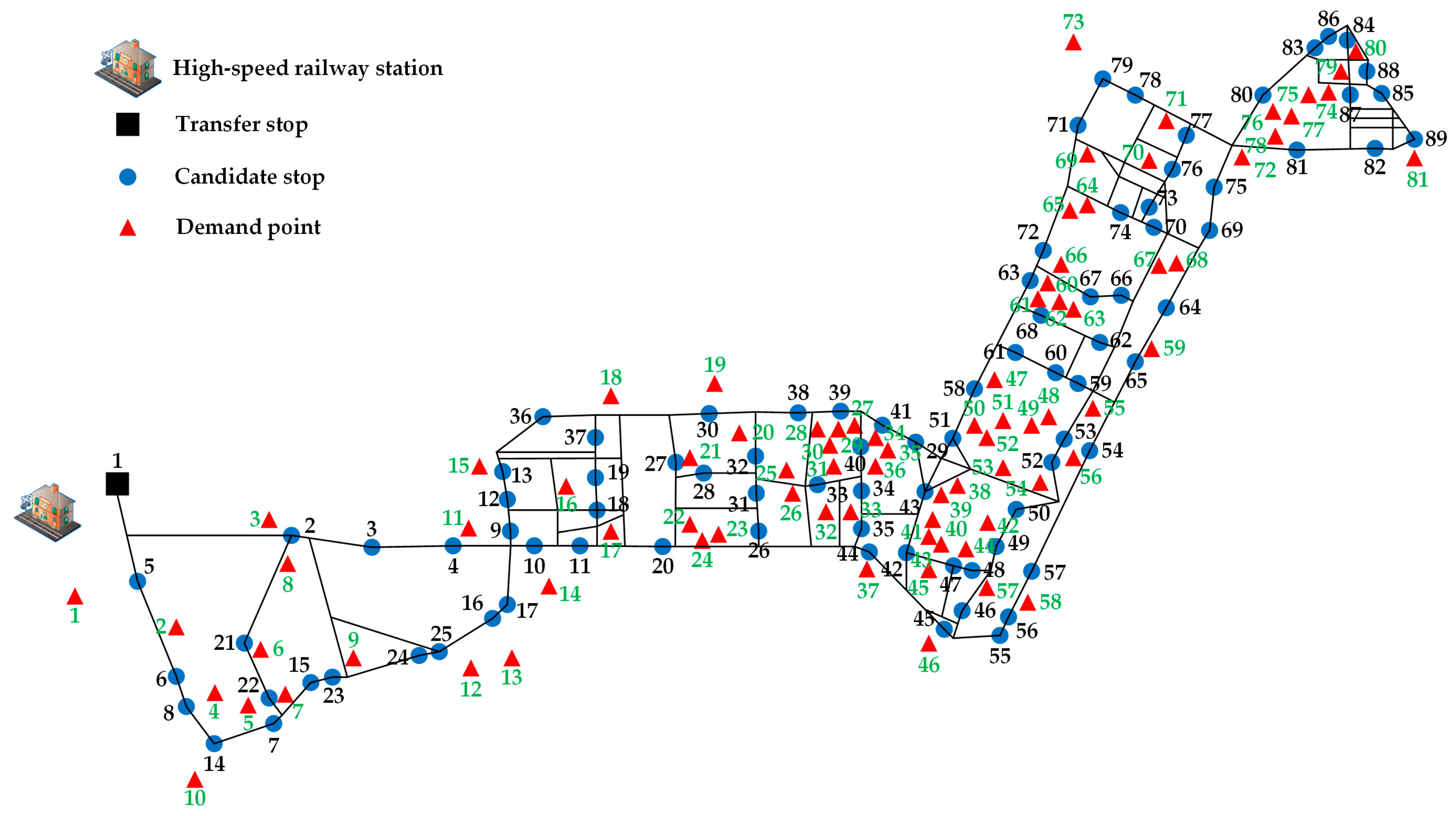
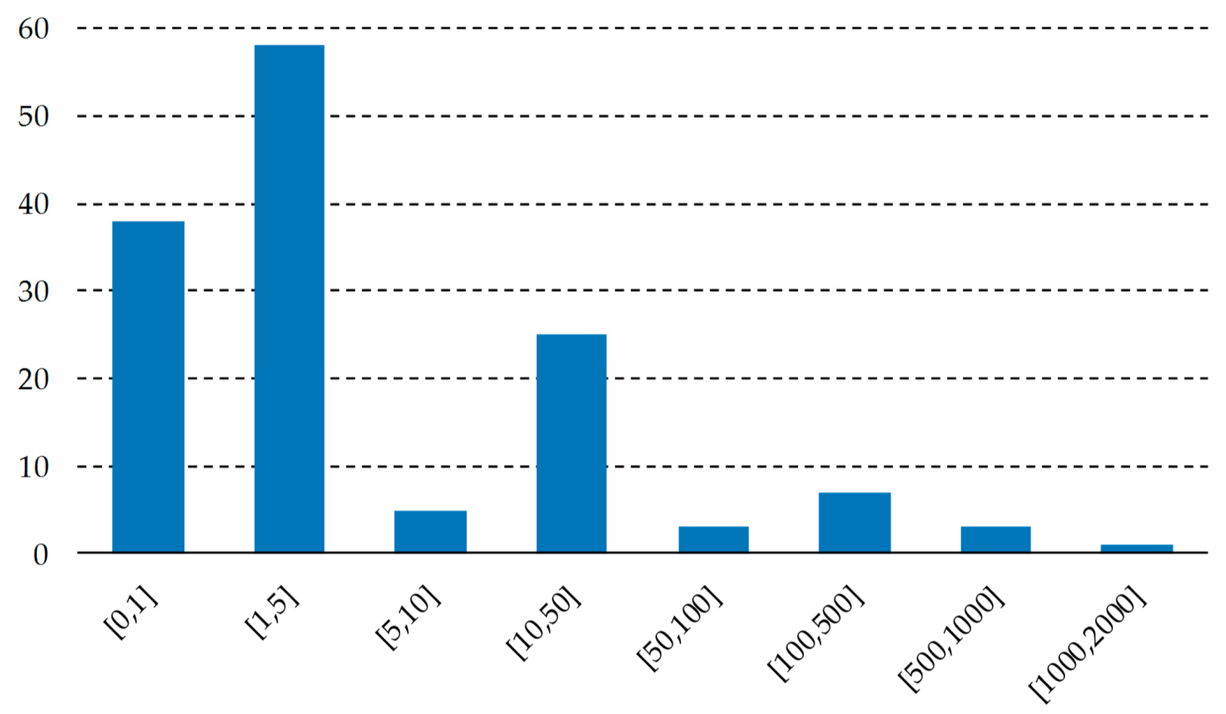
5.1. Scenario Studied

Figure 2 presents the road network of the numerical example. A transfer stop (No. 1) is located near a high-speed rail station. Moreover, there are 88 candidate stops (No. 2–89) and 81 demand points (No. 1–81) in the study area. Tables S1–S4 (see the supplemental files) present the values of the assistant parameters a_ik, the distances between the candidate stops d_kl, the straight-line distances between the transfer stop and candidate stops ${\overline{d}}_k$ and the travel demand q_i, respectively.

In addition, we assume that the maximum and minimum lengths of the feeder bus route (l_max and l_min) are 12 km and 8 km, respectively. The maximum and minimum values of the stop spacing (s_max and s_min) are 1300 m and 500 m, respectively. The maximum nonlinear factor c is 1.4. The maximum acceptable walking distance of passengers D_max equals to 500 m. The assumed values above are reasonable to our knowledge and mostly derived from a design code of China, i.e., “Code for transport planning on urban road” (GB50220-95). These values are only used as an illustrative example here and certainly can be modified according to specific needs of planners (or researchers) or to test other scenarios.

5.2. Computational Results

We implemented all tests on an Intel Core (TM) i5 CPU at 2.27 GHz under Windows 7 with 4 GB of RAM. Each single-objective optimization sub-problem is solved by ILOG CPLEX 12.4.

The Pareto optimal front of the numerical example is shown in Figure 3. The computation time is 753.88 s. Given that the numerical example is on an actual size scale and that we are in the planning stage, this amount of computing time is reasonable. As shown in Figure 3, there are 36 Pareto optimal solutions. An examination of the relationship between the Pareto optimal solutions’ objective values suggests that the longer the feeder bus route length, the more travel demand can be served. This indicates that we choose two conflicting objectives, considering that the feed er bus route length is a minimized objective and the travel demand that can be served is a maximized one. Therefore, the two objectives are reasonable for multi-objective optimization. The feeder bus routes, travel demand that can be served and route length corresponding to each obtained Pareto optimal solution are listed in

Table 3. Results of the Pareto optimal solutions.

Solution	Route	Travel Demand That Can Be Served (trip/day)	Route Length (m)
1	1-2-4-11-19-27-32-33-40-29	10,914	8000
2	1-2-3-10-20-26-33-40-44-51	11,098	8001
3	1-2-4-11-26-32-33-43-42-48	12,813	8002
4	1-2-3-4-9-11-20-26-33-40-35-43-58	13,204	8010
5	1-2-4-10-20-26-33-43-58-68	14,027	8042
6	1-2-4-10-20-26-33-35-43-58-68	14,470	8252
7	1-2-3-4-10-20-26-33-40-29-58-68	14,654	8304
8	1-2-4-10-20-26-32-33-43-58-68	14,676	8460
9	1-2-4-11-26-33-40-51-42-48	14,771	8468
10	1-2-3-10-20-26-33-40-43-58-68	15,591	8520
11	1-2-3-4-11-20-26-33-43-58-68-72	15,831	8634
12	1-2-3-4-10-20-26-33-40-35-43-58-68	16,034	8730
13	1-2-3-10-20-26-33-35-43-58-68-72	16,274	8844
14	1-2-4-10-20-26-33-40-29-58-68-72	16,458	8896
15	1-2-4-11-20-26-32-33-43-58-68-72	16,480	9052
16	1-5-2-4-11-20-26-33-40-43-58-68	16,613	9094
17	1-2-4-11-20-26-33-40-43-58-68-72	17,395	9112
18	1-2-3-4-11-26-33-40-35-43-58-68-72	17,838	9322
19	1-2-4-10-20-26-32-33-40-43-58-68-72	18,044	9530
20	1-5-2-4-11-26-33-40-43-58-68-72	18,417	9686
21	1-2-4-11-26-32-33-40-35-43-58-68-72	18,487	9740
22	1-2-3-4-11-26-33-40-42-43-58-68-72	18,634	9754
23	1-5-2-3-10-20-26-33-40-35-43-58-68-72	18,860	9896
24	1-2-3-4-11-20-26-32-33-40-43-58-68-72-73	18,879	10,612
25	1-2-4-11-26-33-40-42-43-58-68-72-71	18,951	10,636
26	1-5-2-3-4-11-20-26-33-40-43-58-68-72-73	19,252	10,768
27	1-2-3-4-10-20-26-32-33-40-35-43-58-68-72-73	19,322	10,822
28	1-2-4-11-26-33-40-42-43-58-68-72-73	19,469	10,836
29	1-5-2-3-4-10-20-26-33-40-35-43-58-68-72-73	19,695	10,978
30	1-5-2-3-10-20-26-33-40-43-58-68-72-73-69	19,771	11,389
31	1-2-4-10-20-26-32-33-40-35-43-58-68-72-73-69	19,841	11,443
32	1-2-3-4-11-26-33-40-42-43-58-68-72-73-69	19,988	11,457
33	1-5-2-4-10-20-26-33-40-35-43-58-68-72-73-77	20,078	11,648
34	1-2-3-4-11-26-33-40-43-58-68-72-73-77-81	20,139	11,655
35	1-2-4-11-26-33-40-35-43-58-68-72-74-77-81	20,332	11,846
36	1-2-4-11-20-26-33-40-35-43-58-68-72-73-77-81	20,582	11,865

.

Table 4. Situation of matching demand points to candidate stops.

Solution	Situation of Matching Demand Points to Candidate Stops 1
1	(3,8)-2,11-4,(16,18)-19,17-11,(20,25,26)-32,(21,22)-27,(25,26,28,30,31,32,33)-33,(27,34,35,39,40)-29,(27,31,34,36)-40
12	8-3,11-4,11-10,17-20,(23,24)-26,(25,26,28,30,31,32,33)-33,(27,31,34,36)-40,(33,37)-35,(38,39,40,41)-43,(47,50,51,52)-58,(60,61,62,63)-68
19	(3,8)-2,11-4,11-10,17-20,(20,25,26)-32,(23,24)-26,(25,26,28,30,31,32,33)-33,(27,31,34,36)-40,(38,39,40,41)-43,(47,50,51,52)-58,(60,61,62,63)-68,(60,64,65,66)-72
23	(1,2)-5,(3,8)-2,8-3,11-4,17-11,(23,24)-26,(25,26,28,30,31,32,33)-33,(27,31,34,36)-40,(33,37)-35,(38,39,40,41)-43,(47,50,51,52)-58,(60,61,62,63)-68,(60,64,65,66)-72
29	(1,2)-5,(3,8)-2,11-4,17-11,(23,24)-26,(25,26,28,30,31,32,33)-33,(27,31,34,36)-40,(33,37)-35,(38,39,40,41)-43,(47,50,51,52)-58,(60,61,62,63)-68,(60,64,65,66)-72,(67,70)-73
36	(3,8)-2,11-4,17-11,17-20,(23,24)-26,(25,26,28,30,31,32,33)-33,(27,31,34,36)-40,(33,37)-35,(38,39,40,41)-43,(47,50,51,52)-58,(60,61,62,63)-68,(60,64,65,66)-72,(67,70)-73,(70,71)-77,(72,78)-81

¹ The numbers before “-“ represent demand points, and the numbers behind “-“ denote candidate stops. For example, “11-4” means that the eleventh demand point can be served by the forth candidate stop, and “(3,8)-2” means that the third and eighth demand points are served by the second candidate stop.

shows the match situation of demand points and stops. Limited by space, we only present the match situation of six solutions. Figure 4 shows the locations of stops and the feeder bus route of Solution 36 visually.

5.3. Effect of the Maximum Acceptable Walking Distance of Passengers

The maximum acceptable walking distance of passengers is a significant parameter related to the travel demand that can be served and can influence the feeder bus route length. This parameter also determines the assistant parameter a_ik. We change the maximum acceptable walking distance of passengers between 300 m and 500 m. The Pareto optimal solutions in different cases (the maximum acceptable walking distance of passengers D_max is set to 300 m, 350 m, 400 m, 450 m, and 500 m, respectively) for this numerical example are presented in Figure 5.

As presented in Figure 5, as the maximum acceptable walking distance of passengers D_max increases from 300 m to 500 m, the Pareto optimal curves move from bottom to top. This result indicates that increasing this parameter means that more travel demand can be served, when the route length does not change much. Because when D_max is increasing, the number of demand points that can be served by each stop may increase, and certainly will not decrease. Since stop spacing is kept within a certain range, if route length does not change much, the number of stops visited will remain within a certain range. In addition, stops can only be selected from a few candidate stops, so the number of stops for feeder bus routes with similar lengths will not change much. Consequently, for feeder bus routes with similar lengths, as the maximum acceptable walking distance increases, the travel demand that can be served increases. That is, more travel demand can be served when the maximum acceptable walking distance increases while the route length does not change much.

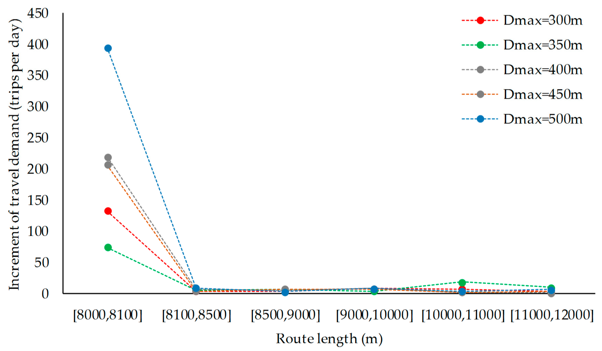
5.4. Benefits Brought by Increasing Feeder Bus Route Length

Then, we analyze benefits brought by increasing the feeder bus route length. Figure 6 shows the travel demand benefited by adding 1 km to the feeder bus route, considering all solutions shown in Figure 5. To obtain this histogram, we calculate the variations of each objective for two adjacent solutions in Figure 5. Then the variations of objective C₁ are divided by the variations of objective C₂. The above calculation process is shown in Equation (17).

$$R_m^n=\frac{C_{1,m+1}^n-C_{1,m}^n}{C_{2,m+1}^n-C_{2,m}^n},$$

(17)

where n = 1, 2, 3, 4, and 5 represent situations that the maximum acceptable walking distances are 300 m, 350 m, 400 m, 450 m, and 500 m respectively; $R_m^n$ is the mth value of increased travel demand that can be served by adding 1 km to feeder bus route in the nth case; $C_{1,m}^n$ is the value of objective C₁ of the mth Pareto optimal solution in the nth case; $C_{2,m}^n$ is the value of objective C₂ of the mth Pareto optimal solution in the nth case. The horizontal axis shows the intervals of increased travel demand that can be served by adding 1 km to the feeder bus route and the vertical axis shows their frequency. As we can see, adding 1 km to the feeder bus route often bring small benefits for most cases. However, there are some cases where adding 1 km to the feeder bus route can result in more than 100 additional trips that can be served.

To know in which range of route length, increasing the feeder bus route length is more efficient, we calculate the average increased travel demand that can be served by adding 1 km to the feeder bus route when the feeder bus route length is in different ranges, considering all solutions, shown in Figure 5. The increased travel demand by adding 1 km to the feeder bus route is also calculated according to Equation (17). As shown in Figure 7, the average increased travel demand that can be served by adding 1 km to the feeder bus route is significantly larger when the feeder bus route length is between 8000 m and 8100 m than when the feeder bus route length is in other intervals. This conclusion is suitable for all cases of the maximum acceptable walking distance. Hence, when the feeder bus route length is between 8000 m and 8100 m, adding 1 km to feeder bus route is the most efficient.

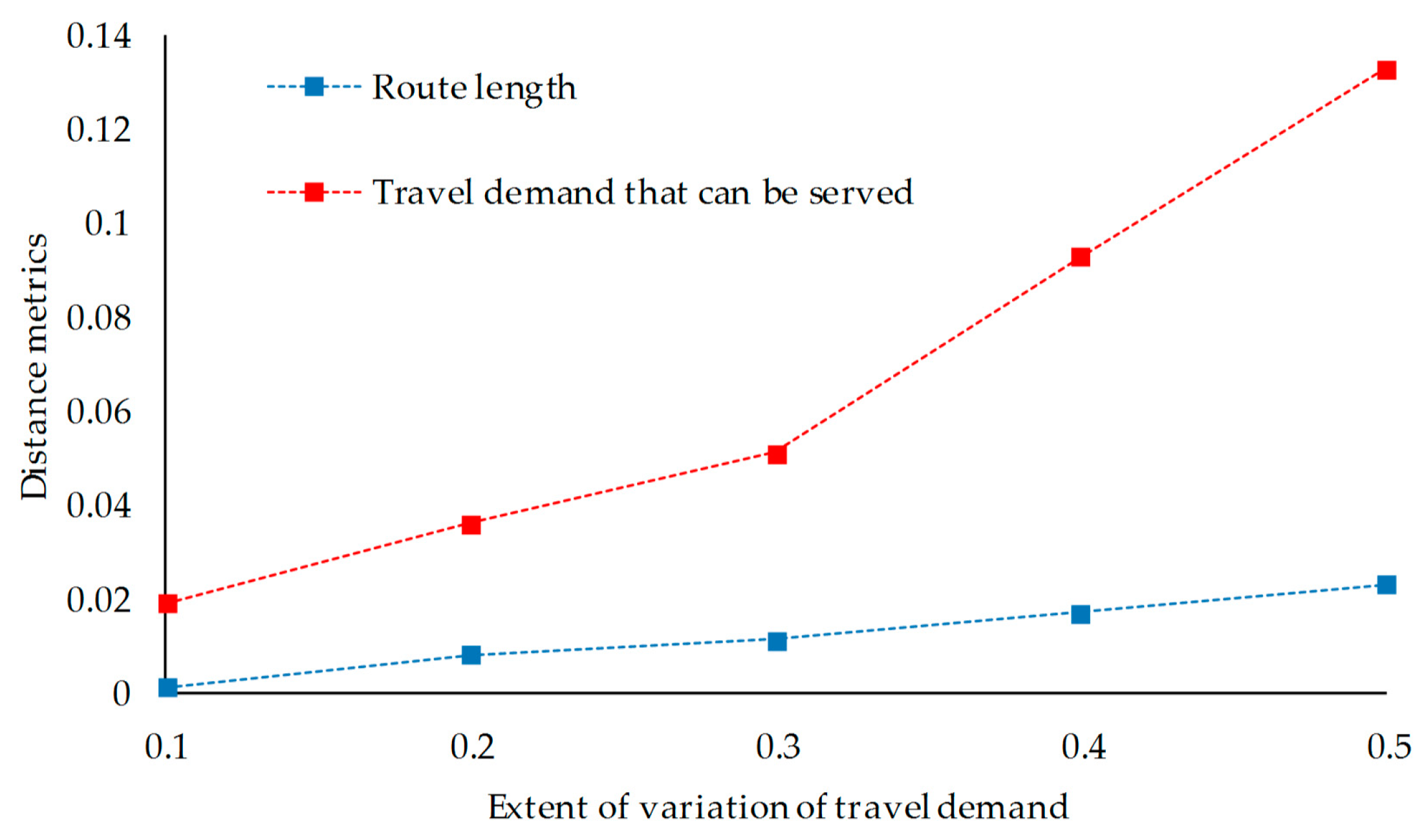
5.5. Robustness of the Pareto Optimal Solutions

For the convenience of passengers and operators, it is often not possible to adjust the stop location and route of the urban public transport system frequently. However, the travel demand may change every day. Considering the fluctuation of high-speed railway passenger volume, especially the difference of passenger volume between workdays and holidays, this character is particularly obvious for the feeder bus service for high-speed rail stations. Therefore, it is necessary to evaluate the robustness of the Pareto optimal solutions. For the scenario shown in Section 5.1, we generate the travel demand of each demand point from a uniform distribution [(1 − α) × q_i, (1 + α) × q_i], where α is the variation extent of travel demand q_i. To evaluate the effect of α on the robustness of the Pareto optimal solutions, we set α to 10%, 20%, 30%, 40% and 50%, respectively. For each case of α, 100 travel demand matrices are generated randomly, which means that 100 Pareto optimal fronts is generated for each situation of α. To measure the robustness of the obtained Pareto optimal solutions, we design the following distance metric to indicate the maximum “distance” between all the Pareto optimal fronts for each case of α:

$$d_t^b=\underset{\forall p,q\in R_t,p\ne q}{\max }{d}_{pq}^b,$$

(18)

where $d_t^b$ is the distance metric value of the bth objective for the tth case of α; R_t is the set of Pareto optimal fronts for the tth case of α; $d_{pq}^b$ is the distance metric value of the bth objective between the pth Pareto optimal front F_p and the qth Pareto optimal fronts F_q of R_t and is defined by

$$d_{pq}^b=\frac{1}{\left|F_p\right|+\left|F_q\right|}\left({\displaystyle \sum _{r\in F_p}\underset{s\in F_q}{\min }{d}^b\left(r,s\right)}+{\displaystyle \sum _{s\in F_q}\underset{r\in F_p}{\min }{d}^b\left(s,r\right)}\right),$$

(19)

where d^b(r,s) is defined as follows.

$$d^b\left(r,s\right)=\left|\frac{1}{{\Delta }_b}\left(f_b\left(r\right)-f_b\left(s\right)\right)\right|,$$

(20)

where f_b(r) and f_b(s) are the values of the bth objective of solution r and solution s, respectively; Δ_b is the range of the bth objective among all solutions in F_p and F_q.

Figure 8 shows the distance metric values of objective C₁ and C₂. Compared with C₂, the distance metric values of C₁ are larger. This means that the fluctuation of travel demand has a greater impact on C₁. This is because some fluctuations of travel demand cannot influence the optimality of the feeder bus route, while they usually influence the travel demand that can be served. It can also be seen that when α increases, the distance metric values of objective C₁ and C₂ increase. Compared with C₁, the distance metric values of C₂ increase more slowly, which indicates that the robustness of the feeder bus route will be less affected by an increase of α. The distance metric values of C₁ are relatively less when α = 10%, 20% and 30%, which means that when α is not more than 30%, the passenger volume of the feeder bus system is relatively stable. However, if the variation extent of travel demand exceeds 30%, the passenger volume of the feeder bus system may have a larger fluctuation.

5.6. Integrated Approach vs. Exisiting Approach

An existing approach is to first decide terminals and bus routes, then other bus stops are set along the bus routes [42,43]. To compare our integrated approach and the existing approach, we divide the formulation in Section 3 and solve the bus stop location and route design sequentially. The existing approach is described in detail below.

First, we only decide the bus route and consider the candidate stops in Section 5.1 as candidate terminals. Formulation M1 is used to design the bus route. The sets, parameters and decision variables used in M1 are presented in

Table 5. Sets, parameters and decision variables in M1.

Sets
N	set of demand nodes, $m,n\in N$
N′	set of candidate terminals, $N^{\prime }\subseteq N$
A	set of road links, $\left(m,n\right)\in A,m,n\in N$
Parameters
$d_{mn}^{\prime }$	length of road links (m,n)
${\overline{d}}_m^{\prime }$	straight-line distance between the transfer stop and candidate terminals m
Decision variables
wmn	a binary variable (1 if road link (m,n) belongs to the route and 0 otherwise)
$x_m^{\prime }$	a binary variable which equals 1 if the route passes node m, and 0 otherwise
$u_m^{\prime }$	a nonnegative integer assistant variable to eliminate sub-tour

.

Other parameters used in M1 have been defined in Section 3.2. M1 can be described as follows.

M1:

$$\min C_2^{\prime }={\displaystyle \sum _{\left(m,n\right)\in A,n\ne 1}{w}_{mn}{d}_{mn}^{\prime }},$$

(21)

subject to

$$l_{\min }\le {\displaystyle \sum _{\left(m,n\right)\in A,n\ne 1}{w}_{mn}{d}_{mn}^{\prime }}\le l_{\max },$$

(22)

$${\displaystyle \sum _{\left(m,n\right)\in A,n\ne 1}{w}_{mn}{d}_{mn}^{\prime }}\le c{\displaystyle \sum _{m\in N^{\prime }}{w}_{m1}{\overline{d}}_m^{\prime }},$$

(23)

$$\begin{array}{cc}{\displaystyle \sum _{n\in N,n\ne m}{w}_{mn}}={\displaystyle \sum _{n\in N,n\ne m}{w}_{nm}}=x_m^{\prime },& \forall m\in N,\end{array}$$

(24)

$$x_1^{\prime }=1,$$

(25)

$$\begin{array}{cc}{u}_m-u_n+\left|N\right|w_{mn}\le \left|N\right|-1,& \forall m,n\in N,n\ne 1,n\ne m,\end{array}$$

(26)

$$\begin{array}{cc}{w}_{mm}=0,& \forall m\in N,\end{array}$$

(27)

$$\begin{array}{cc}{w}_{m1}=0,& \forall m\in N\backslash N^{\prime },\end{array}$$

(28)

$$\begin{array}{cc}{x}_m^{\prime },w_{mn}\in \left\{0,1\right\},& \forall m,n\end{array}\in N,$$

(29)

$$\begin{array}{cc}{u}_m\ge 0,& \forall m\in N,\end{array}$$

(30)

The objective (21) is to minimize the route length. Constraint (22) represents the minimum and maximum lengths of the feeder bus route. Constraint (23) ensures that the nonlinear factor of the feeder bus route does not exceed the maximum nonlinear factor. Constraint (24) defines the degrees of nodes and ensures the flow conservation at nodes. Constraint (25) guarantees that the transfer stop is passed by the route. Due to Constraint (26), the sub-tour is avoided. Constraint (27) ensures that each node is not passed twice by the route. Constraint (28) states that the feeder bus route cannot end at a node, which is not a candidate terminal. Constraints (29)–(30) define the domains of the decision variables.

Second, all candidate stops along the feeder bus route generated and demand points are considered. The optimal stops are found and the situation of matching the demand points to the stops is decided. To this end, we establish formulation M2 as follows.

M2:

max C₁

subject to

$$\begin{array}{cc}{z}_{kl}{s}_{\min }\le z_{kl}{d}_{kl}\le z_{kl}{s}_{\max },& \forall k,l\in \overline{H},l\ne 1,\end{array}$$

(31)

$$\begin{array}{cc}{x}_k\cdot a_{ik}=y_{ik},& \forall i\in D,k\in \overline{H},\end{array}$$

(32)

$$\begin{array}{cc}{\displaystyle \sum _{i\in D}{y}_{ik}}\ge x_k,& \forall k\in \overline{H},k\ne 1,\end{array}$$

(33)

$$\begin{array}{cc}{\displaystyle \sum _{l\in \overline{H},l\ne k}{z}_{kl}}={\displaystyle \sum _{l\in \overline{H},l\ne k}{z}_{lk}}=x_k,& \forall k\in \overline{H},\end{array}$$

(34)

x₁ = 1,

(35)

$$\begin{array}{cc}{u}_k-u_l+\left|\overline{H}\right|z_{kl}\le \left|\overline{H}\right|-1,& \forall k,l\in \overline{H},l\ne 1,l\ne k,\end{array}$$

(36)

$$\begin{array}{cc}{z}_{kk}=0,& \forall k\in \overline{H},\end{array}$$

(37)

$$\begin{array}{cc}{v}_i\le {\displaystyle \sum _{k\in \overline{H}}{y}_{ik}},& \forall i\in D,\end{array}$$

(38)

$$\begin{array}{cc}{v}_i\ge y_{ik},& \forall i\in D,k\in \overline{H},\end{array}$$

(39)

$$\begin{array}{cc}{v}_i,x_k,y_{ik},z_{kl}\in \left\{0,1\right\},& \forall k,l\in \overline{H},i\in D,\end{array}$$

(40)

$$\begin{array}{cc}{u}_k\ge 0,& \forall k\in \overline{H},\end{array}$$

(41)

$$w_{m^{\prime }1}=1,$$

(42)

$${\displaystyle \sum _{k\in \overline{H}}{\displaystyle \sum _{l\in \overline{H},l\ne 1}{z}_{kl}{d}_{kl}}}=C_2^{\prime },$$

(43)

where $\overline{H}$ is the set of candidate stops along the feeder bus route generated by solving M1; $m^{\prime }\in \overline{H}$ is the terminal of the feeder bus route generated by solving M1; $C_2^{\prime }$ is the length of the feeder bus route generated by solving M1. Other sets, parameters and decision variables have been presented in Table 2.

We also decide the feeder bus route in M2, because the decision variable z_kl can describe stop spacing. Since we only consider the candidate stops along the feeder bus route generated by solving M1 and restrain the terminal and length, the feeder bus route generated by M2 is the same as the feeder bus route generated by M1. Obviously, the feeder bus route decision will not affect the stop location. Notice that the maximum stop spacing s_max and minimum stop spacing s_min may need to be modified to make M2 feasible, because the minimum and maximum bus stop spacing constraints are not taken into account in M1.

We use the existing approach to solve the stop location and route design problem for the scenario in Section 5.1 and the maximum stop spacing is modified to 1400 m. The generated feeder bus route and stops are shown in Figure 9. The length of this feeder bus route is 8000 m and the travel demand that can be served is 8109 trips/day. The situation of matching demand points to stops is presented in

Table 6. Match situation of demand points and stops for the solution of the existing approach.

Solution	Situation of Matching Demand Points to Candidate Stops 1
The solution of the existing approach	(3,8)-2,11-4,11-9,(16,17)-18,(16,18)-37,19-30,(27,28,29,30)-38,(27,34,35)-41,(38,39,40,41)-43

¹ The numbers before “-“ represent demand points, and the numbers behind “-“ denote candidate stops. For example, “11-4” means that the eleventh demand point can be served by the forth candidate stop, and “(3,8)-2” means that the third and eighth demand points are served by the second candidate stop.

.

As we can see, the route length of the solution generated by the existing approach is the same as the route length of Solution 1, shown in Table 3. While the travel demand that can be served of the solution generated by the existing approach is less than the travel demand that can be served of Solution 1. This is reasonable. The travel demand is ignored in the first step of the existing approach and only the route length is optimized. The route length of the solution generated by the existing approach is minimized. However, the feeder bus routes with the same route length while serve more travel demand may not be generated by the existing approach. For our integrated approach, the travel demand and route length are both considered. Thus, the feeder bus routes with the same route length while serve more travel demand can be obtained. Moreover, considering the trade-off between objectives, more than one solution may be obtained by our approach. Whereas, the existing approach can only generate one solution.

In other words, considering both travel demand and route length, our integrated approach can generate better and more solutions than the existing approach.

6. Conclusions

The feeder bus is a main feeder transportation mode for high-speed railway passengers. Planners must solve the problem of how to design feeder bus routes for high-speed rail stations properly. We proposed a bi-objective mathematical model and an exact ε-constraint method were developed to assist planners in this decision-making process. The maximum acceptable walking distance of passengers is considered in the mathematical formulation and the Pareto optimal solutions can be obtained within reasonable time.

Based on the mathematical formulation and solution method, planners can obtain feeder bus routes and stop locations simultaneously. In this way, a critical trade-off is made between two objectives: Travel demand that can be served and route length. A numerical example on an actual size scale is used to verify the proposed approach. Through the sensitivity analysis of the maximum acceptable walking distance of passengers, we have shown that the longer maximum acceptable walking distance of passengers will result in more travel demand being served, when the route length does not change a lot. Moreover, when the route length is between 8000 m and 8100 m, increasing the feeder bus route length is more efficient for increasing the travel demand that can be served. To elucidate the robustness of the generated solutions, some tests are executed based on randomly generated travel demand matrices. The results indicate that the robustness of obtained feeder bus routes will not be influenced much under different extents of travel demand fluctuation. Finally, compared with the existing approach, our approach can generate better solutions.

A further research area is to consider headway when designing feeder bus routes for high-speed rail stations. Headway concerns both the passenger and operator cost. The integrated design of the route and headway of the feeder bus service for high-speed rail stations should make the feeder bus system perform better. In addition, establishing a formulation to consider the effect of congestion is also an interesting work.

References

1. Semler, C.; Hale, C. Rail station access—An assessment of options. In Proceedings of the 33rd Australasian Transport Research Forum Conference, Canberra, Australia, 29 Semptember–1 October 2010. [Google Scholar]
2. Cheng, X.Y.; Cao, Y.; Huang, K.; Wang, Y.J. Modeling the satisfaction of bus traffic transfer service quality at a high-speed railway station. J. Adv. Transp. 2018, 2018, 7051789:1–7051789:12. [Google Scholar] [CrossRef]
3. Teng, J.; Shen, B.; Fei, X.; Zhang, J.X.; Jiang, Z.B.; Ma, C. Designing feeder bus lines for high-speed railway terminals. Syst. Eng. Theory Pract. 2013, 33, 2937–2944. [Google Scholar] [CrossRef]
4. Fan, W. Optimal transit route network design problem: Algorithms, implementations, and numerical results. Ph.D. Thesis, The University of Texas at Austin, Austin, TX, USA, 2004. [Google Scholar]
5. Park, J.; Kim, B.I. The school bus routing problem: A review. Eur. J. Oper. Res. 2010, 202, 311–319. [Google Scholar] [CrossRef]
6. Metcalf, D.D.; Bond, V.L. Bus stop guidelines to meet urban, suburban and rural conditions. In Proceedings of the ITE 2006 Technical Conference and Exhibit Compendium of Technical Papers, San Antonio, TX, USA, 19–22 March 2006. [Google Scholar]
7. Chien, S.; Yang, Z.W. Optimal feeder bus routes on irregular street networks. J. Adv. Transpt. 2000, 34, 213–248. [Google Scholar] [CrossRef]
8. Jerby, S.; Ceder, A. Optimal routing design for shuttle bus service. In Proceedings of the 85th Annual Meeting of the Transportation-Research-Board, Transportation Research Board Natl Research Council, Washington, DC, USA, 22–26 January 2006. [Google Scholar] [CrossRef]
9. Xiong, J.; Guan, W.; Huang, A.L. Research on optimal routing of community shuttle connect rail transit line. J. Trans. Syst. Eng. Inf. Technol. 2014, 14, 166–173. [Google Scholar] [CrossRef]
10. Zhu, Z.J.; Guo, X.C.; Zeng, J.; Zhang, S.R. Route design model of feeder bus service for urban rail transit stations. Math. Probl. Eng. 2017, 2017, 1090457:1–1090457:6. [Google Scholar] [CrossRef]
11. Pan, S.L.; Yu, J.; Yang, X.F.; Liu, Y.; Zou, N. Designing a flexible feeder transit system serving irregularly shaped and gated communities: Determining service area and feeder route planning. J. Urban Plan. Dev. 2014, 141, 04014028:1–04014028:9. [Google Scholar] [CrossRef]
12. Lin, J.J.; Wong, H.I. Optimization of a feeder-bus route design by using a multiobjective programming approach. Transpt. Plan. Technol. 2014, 37, 430–449. [Google Scholar] [CrossRef]
13. Shrivastava, P.; Dhingra, S.L. Development of feeder routes for suburban railway stations using heuristic approach. J. Transp. Eng. 2001, 127, 334–341. [Google Scholar] [CrossRef]
14. Kuan, S.N.; Ong, H.L.; Ng, K.M. Applying metaheuristics to feeder bus network design problem. Asia Pac. J. Oper. Res. 2004, 21, 543–560. [Google Scholar] [CrossRef]
15. Kuan, S.N.; Ong, H.L.; Ng, K.M. Solving the feeder bus network design problem by genetic algorithms and ant colony optimization. Adv. Eng. Softw. 2006, 37, 351–359. [Google Scholar] [CrossRef]
16. Shrivastava, P.; O’ Mahony, M. A model for development of optimized feeder routes and coordinated schedules—A genetic algorithms approach. Transp. Policy 2006, 13, 413–425. [Google Scholar] [CrossRef]
17. Shrivastava, P.; O’ Mahony, M. Use of a hybrid algorithm for modeling coordinated feeder bus route network at suburban railway station. J. Transp. Eng. 2009, 135, 1–8. [Google Scholar] [CrossRef]
18. Song, R.; Liu, Z.Q. Heuristic algorithm for feeder bus route generation in railway traffic system. J. Jilin Univ. 2011, 41, 1234–1239. [Google Scholar]
19. Sun, Y.; Song, R.; He, S.W. Feeder bus network design under elastic demand. J. Jilin Univ. 2011, 41, 349–354. [Google Scholar] [CrossRef]
20. Szeto, W.Y.; Wu, Y.Z. A simultaneous bus route design and frequency setting problem for Tin Shui Wai, Hong Kong. Eur. J. Oper. Res. 2011, 209, 141–155. [Google Scholar] [CrossRef] [Green Version]
21. Liu, H.S.; Zhao, S.Z.; Zhu, Y.G.; Li, X.Y. Feeder bus network design model based on effective path. J. Jilin Univ. 2015, 45, 371–378. [Google Scholar] [CrossRef]
22. Perugia, A.; Moccia, L.; Cordeau, J.F.; Laporte, G. Designing a home-to-work bus service in a metropolitan area. Transp. Res. B Methodol. 2011, 45, 1710–1726. [Google Scholar] [CrossRef]
23. Li, H.G.; Chen, Y.S. Study on enterprise shuttle bus location and route optimization: An integrated approach. J. Univ. Electron. Sci. Technol. China 2016, 18, 68–73. [Google Scholar] [CrossRef]
24. Leksakul, K.; Smutkupt, U.; Jintawiwat, R.; Phongmoo, S. Heuristic approach for solving employee bus routes in a large-scale industrial factory. Adv. Eng. Inf. 2017, 32, 176–187. [Google Scholar] [CrossRef]
25. Xiong, J.; Guan, W.; Song, L.Y.; Huang, A.L.; Shao, C.F. Optimal routing design of a community shuttle for metro stations. J. Transp. Eng. 2013, 139, 1211–1223. [Google Scholar] [CrossRef]
26. Schittekat, P.; Kinable, J.; Sorensen, K.; Sevaux, M.; Spieksma, F.; Springael, J. A metaheuristic for the school bus routing problem with bus stop selection. Eur. J. Oper. Res. 2013, 229, 518–528. [Google Scholar] [CrossRef]
27. Chen, J.X.; Wang, S.A.; Liu, Z.Y.; Wang, W. Design of suburban bus route for airport access. Transp. A Transp. Sci. 2017, 13, 568–589. [Google Scholar] [CrossRef]
28. Yan, S.Y.; Wang, S.S.; Wu, M.W. A model with a solution algorithm for the cash transportation vehicle routing and scheduling problem. Comput. Ind. Eng. 2012, 63, 464–473. [Google Scholar] [CrossRef]
29. Yan, S.Y.; Wang, S.S.; Chang, Y.H. Cash transportation vehicle routing and scheduling under stochastic travel times. Eng. Optimiz. 2014, 46, 289–307. [Google Scholar] [CrossRef]
30. Bányai, T. Real-time decision making in first mile and last mile logistics: How smart scheduling affects energy efficiency of hyperconnected supply chain solutions. Energies 2018, 11, 1833. [Google Scholar] [CrossRef]
31. Bányai, T.; Illés, B.; Bányai, Á. Smart scheduling: An integrated first mile and last mile supply approach. Complexity 2018, 2018, 5180156:1–5180156:15. [Google Scholar] [CrossRef]
32. Zhou, L.; Baldacci, R.; Vigo, D.; Wang, X. A multi-depot two-echelon vehicle routing problem with delivery options arising in the last mile distribution. Eur. J. Oper. Res. 2018, 265, 765–778. [Google Scholar] [CrossRef]
33. Ramos, T.R.P.; Morais, C.S.D.; Barbosa-Póvoa, A.P. The smart waste collection routing problem: Alternative operational management approaches. Expert Syst. Appl. 2018, 103, 146–158. [Google Scholar] [CrossRef]
34. Tirkolaee, E.B.; Mahdavi, I.; Esfahani, M.M.S. A robust periodic capacitated arc routing problem for urban waste collection considering drivers and crew’s working time. Waste Manag. 2018, 76, 138–146. [Google Scholar] [CrossRef]
35. Bányai, T.; Tamás, P.; Illés, B.; Stankevičiūtė, Ž.; Bányai, Á. Optimization of municipal waste collection routing: Impact of industry 4.0 technologies on environmental awareness and sustainability. Int. J. Environ. Res. Public Health. 2019, 16, 634. [Google Scholar] [CrossRef]
36. Riedler, M.; Raidl, G. Solving a selective dial-a-ride problem with logic-based Benders decomposition. Comput. Oper. Res. 2018, 96, 30–54. [Google Scholar] [CrossRef]
37. Tellez, O.; Vercraene, S.; Lehuédé, F.; Péton, O. The fleet size and mix dial-a-ride problem with reconfigurable vehicle capacity. Transp. Res. C Emerg. Technol. 2018, 91, 99–123. [Google Scholar] [CrossRef] [Green Version]
38. Chen, C.; Zhang, D.Q.; Li, N.; Zhou, Z.H. B-planner: Planning bidirectional night bus routes using large-scale taxi GPS traces. IEEE Trans. Intell. Transp. Syst. 2014, 15, 1451–1465. [Google Scholar] [CrossRef]
39. Huang, C.H.; Galuski, J.; Bloebaum, C.L. Multi-objective Pareto concurrent subspace optimization for multidisciplinary design. AIAA J. 2007, 45, 1894–1906. [Google Scholar] [CrossRef]
40. Berube, J.F.; Gendreau, M.; Potvin, J.Y. An exact ε-constraint method for bi-objective combinatorial optimization problems: Application to the traveling salesman problem with profits. Eur. J. Oper. Res. 2009, 194, 39–50. [Google Scholar] [CrossRef]
41. Deb, K.; Agrawal, S.; Pratap, A.; Meyarivan, T. A fast elitist non-dominated sorting genetic algorithm for multi-objective optimization: NSGA-II. In Proceedings of the Sixth International Conference on Parallel Problem Solving From Nature, Paris, France, 18–20 September 2000. [Google Scholar]
42. Liu, H.D. Research on Bus Transit Routes Network Design Theory and Implement Method. Ph.D. Thesis, Tongji University, Shanghai, China, 2008. [Google Scholar]
43. Yan, P.; Song, R. Urban Public Transit Introduction, 1st ed.; China Machine Press: Beijing, China, 2011; p. 79. [Google Scholar]
Figure 1. Stops and route of the feeder bus service for a high-speed rail station.
Symmetry 11 00514 g001
Figure 2. Road network of the numerical example.
Symmetry 11 00514 g002
Figure 3. Pareto optimal solutions of the numerical example.
Symmetry 11 00514 g003
Figure 4. Stop locations and route of Solution 36.
Symmetry 11 00514 g004
Figure 5. The influence of the maximum acceptable walking distance of passengers.
Symmetry 11 00514 g005
Figure 6. Increased travel demand that can be served by adding 1 km to feeder bus route for all Dmax cases.
Symmetry 11 00514 g006
Figure 7. Average increased travel demand that can be served by adding 1 km to the feeder bus route for different ranges of feeder bus route length.
Symmetry 11 00514 g007
Figure 8. Relationship between extent of variation of travel demand and distance metric value.
Symmetry 11 00514 g008
Figure 9. Stop locations and route of the solution generated by the existing approach.
Symmetry 11 00514 g009