A Fast 4K Video Frame Interpolation Using a Hybrid Task-Based Convolutional Neural Network

Abstract

Visual quality and algorithm efficiency are two main interests in video frame interpolation. We propose a hybrid task-based convolutional neural network for fast and accurate frame interpolation of 4K videos. The proposed method synthesizes low-resolution frames, then reconstructs high-resolution frames in a coarse-to-fine fashion. We also propose edge loss, to preserve high-frequency information and make the synthesized frames look sharper. Experimental results show that the proposed method achieves state-of-the-art performance and performs 2.69x faster than the existing methods that are operable for 4K videos, while maintaining comparable visual and quantitative quality.

1. Introduction

The objective of video frame interpolation is to generate an intermediate frame between temporally adjacent frames for a high frame rate conversion, which is an attempt to make videos more fluid and seamless. Traditional video frame interpolation methods [1,2,3] are mostly based on pixel blending with optical flow estimation. These methods demand precise optical flow estimation in order to achieve good frame interpolation results. Recently, convolutional neural networks, which show impressive performance over various vision tasks, are widely studied for optical flow estimation and video frame interpolation. Many studies have proposed methods that train convolutional neural networks to estimate optical flow fields with ground truth in a supervised fashion [4,5,6,7,8,9]. Liu et al. [10] developed the train pipeline, which implicitly forces a network to estimate better optical flow fields. The accuracy of these methods is largely based on the quality of the optical flow fields, so they tend to have blur or ghost artifacts in the predicted intermediate frames for challenging cases such as occlusion, large motion, and complex structural change. Jiang et al. [11] and Liu et al. [12] proposed a new loss term to enhance the predicted optical flow quality. Jiang et al. [11] proposed a visibility map that excludes the contribution of occluded pixels to the interpolated intermediate frame. Liu et al. [12] proposed cycle consistency loss to enforce the similarity between the input frames and the mapped-back frames. However, these methods still yield poor results for large motion and complex structural change.

To address this problem, Niklaus et al. [13] proposed a pixel-wise frame synthesis method based on spatially adaptive kernels. The trained model predicts N $\times$ N interpolation kernels that capture local motion between input frames. They achieved state-of-the-art performance and showed that it is feasible to combine optical flow estimation and pixel warping in a single step. However, this method has a higher computational complexity and is much more memory intensive because it predicts interpolation kernels for every pixel. Therefore, this method is impossible to perform for high-resolution frames, such as 4K images, due to memory issues. Niklaus et al. [14] approximated 2D kernels with 1D separable kernels for memory efficiency, but they still suffered from expensive computational costs. These methods not only have this problem, but also yield poor interpolation results for high-resolution video frames. The performance of these methods depends mainly on kernel size, and it is necessary to have larger kernels in order to produce good results for large motion. These methods have ghost or blur artifacts for high-resolution video frames since they tend to have larger motion. Niklaus et al. [15] proposed a context-aware synthesis approach that warps not only the input frames but also their pixel-wise contextual information, and uses them to interpolate a high-quality intermediate frame. However, this approach demands much more memory, since the pixel-wise contextual information has same resolution of input frames. Although the majority of video interpolation research [11,12,13,14,15,16,17] has focused on visual and quantitative quality, there are insufficient studies for handling high-resolution video. This is because these methods are memory intensive which is a major obstacle for interpolating high-resolution video frames.

In this paper, we propose a novel hybrid task-based convolutional neural network for the fast and accurate frame interpolation of 4K videos. Our network is composed of a temporal interpolation (TI) network and a spatial interpolation (SI) network, which each have different objectives. The TI network interpolates intermediate frames, which are the same size as the downsampled input frames. The SI network reconstructs original-scale frames from the predicted intermediate frames, similar to super-resolution task [18,19,20,21]. The SI network exploits interpolation feature maps extracted from the TI network using our skip connection. To reduce the number of channels of the interpolation feature maps, we compress them into smaller dimensions, instead of concatenating as in other methods [11,14,22]. Thus, our SI network can remain shallow for good performance. This helps the network become less computational and shortens the inference time. We also propose edge loss to preserve high-frequency information and make the synthesized frames look sharper. The proposed network utilizes the YCbCr420 color format, which is commonly used for video coding as input and output, respectively. Therefore, additional color format converting processes can be omitted using our method for practical application. Consequently, as shown in Figure 1, the proposed method performs faster than the existing state-of-the-art methods that are operable for 4K videos, while maintaining comparable accuracy.

2. Proposed Approach

We propose a hybrid task-based convolutional neural network for frame interpolation. As shown in Figure 2, the proposed network is composed of a TI (temporal interpolation) network and an SI (spatial interpolation) network, each of which has different tasks. The TI network takes downsampled frames as input and interpolates the intermediate frame, which also has a downsampled resolution. This frame is then interpolated by bicubic-interpolation and fed to the SI network. In the SI network, similar to super-resolution, the bicubic interpolated frame is refined in order to improve its visual quality.

Although the YCbCr420 color format is commonly used for video coding, most video frame interpolation methods [10,11,12,14,17] simply use the RGB color domain. The proposed network utilizes the YCbCr420 color format as input and output for both the TI network and the SI network. In YCbCr420 color format, each U or V sample is used to represent four Y samples. That is, for a 4K (2160p) image, Y $\in R^{2160\times 3840}$ while U and V $\in R^{1080\times 1920}$.

2.1. Temporal Interpolation Network

Inspired by [14], we made use of separable convolutional kernels in the TI network. Given two input frames $i_t$, t $\in \left\{0,2\right\}$, the TI network predicts each horizontal and vertical interpolation kernel $k_{t,h}$ and $k_{t,v}$, where $i_t$ is a YCbCr image whose luma channel has the same resolution as its chromas. The luma channel of $i_t$ is downsampled from the luma channel of $I_t$, while the chroma channels of $i_t$ and $I_t$ are identical. To make the proposed method efficient, our TI network estimates low-resolution interpolation kernels. That is, $k_{t,h}\in {\mathit{R}}^{N\times (\frac{H}{2})\times (\frac{W}{2})}$ and $k_{t,v}\in {\mathit{R}}^{N\times (\frac{H}{2})\times (\frac{W}{2})}$, where N is the kernel size, and H and W are the height and width of the chroma image of $I_t$, respectively. We set N = 51 in this paper. The intermediate frame $i_1^{\prime }$ is interpolated, as below.

$$i_1^{\prime }\left(x,y\right)={\displaystyle \sum }_{i\in N}{\displaystyle \sum }_{j\in N}{K}_{0,h}\left(i\right)\times K_{0,v}\left(j\right)\times P_0\left(i,j\right)+K_{2,h}\left(i\right)\times K_{2,v}\times P_2\left(i,j\right)$$

(1)

where, $P_t$ is the local patch centered at $\left(x,y\right)$ in $I_t$. $K_{t,h}$ and $K_{t,v}$ are upsampled interpolation kernels from $k_{t,h}$ and $k_{t,v}$, respectively. Instead of performing upsampling, for memory efficiency, we simply take the adjacent kernel coefficient and calculate the mean value on the fly.

Generally, large amounts of memory are needed to predict these interpolation kernels for high-resolution frames. The interpolation parameters in [14] are $4\times N\times 2H\times 2W$, and it is difficult to predict them for a high-resolution frame simultaneously. For the interpolation kernels, the proposed method has $4\times N\times \frac{H}{2}\times \frac{W}{2}$ parameters, which is 16x less than [14] and enables the interpolation of high-resolution frames such as 4K. The U and V channels of $i_1^{\prime }$ are the output interpolated frame. The Y channel of $i_1^{\prime }$ is interpolated using bicubic-interpolation and fed to the SI network to produce the output Y channel. The spatial interpolation process is described in more detail in Section 2.2.

Our TI network is a fully convolutional neural network composed of an encoder, a decoder, and four sub-networks. There are four skip connections from the encoder layers to the decoder layers and SI network. The encoder has six hierarchical layers, and each hierarchical layer is composed of three convolutional layers followed by an exponential linear unit (ELU) [23] layer and an average pooling layer. We found that using an ELU slightly increases the network accuracy. For the decoder, there are three hierarchical layers with components similar to those of the encoder, except that there is a bilinear upsampling layer at the front of each convolutional layer instead of an average pooling layer. The last layer of decoder is connected to each sub-network. Each sub-network has three convolutional layers followed by a rectified linear unit (ReLU) [24] and a bilinear upsampling layer. We use 3 × 3 kernels in the entire convolutional layers. Overall, our TI network is a variation of u-net [25] architecture.

2.2. Spatial Interpolation Network

The purpose of our SI network is to reconstruct the predicted intermediate frame, which results in higher original resolution. Since this process is similar to the super-resolution task, we first describe several super-resolution methods and then explain the design of our SI network. Kim et al. [18] used very deep convolutional networks, such as VGG-net [26], for single-image super-resolution. They showed that increasing network depth significantly improves reconstruction accuracy compared to existing methods, which have shallow networks. Liao et al. [27] first generated a multi-channel image containing the set of reconstructed blurred images and a bicubic interpolated reference frame. This multi-channel image was used to generate super-resThe number of interpolation parameters in [14] are 4 × N × 2H × 2W. It is difficult to predict the interpolation kernels for a high-resolution frame simultaneouslyolution drafts, which were then combined into a single image. Their method showed that using a multi-channel image guides the network to implicitly learn better super-resolution features. Caballero et al. [28] proposed spatio-temporal sub-pixel convolution networks that exploit temporal redundancies for video frame super-resolution.

The proposed SI network learns to generate $I_{Y\_1}^{″}$ $\in {\mathit{R}}^{2H\times 2W}$ from the input $I_{Y\_t}$ and $I_{Y\_1}^{\prime }$. Here, $I_{Y\_t}$ is the Y channel of the original input frame $I_t$, and $I_{Y\_1}^{\prime }$ is the bicubic interpolated frame from the Y channel of $i_1^{\prime }$. Since our method uses the YcbCr420 color format, the SI network only reconstructs the Y channel. Since the task of the SI network is image reconstruction, using original image information can be a benefit for the quality of the reconstructed image. Using the original image $I_{Y\_t}$ affects the SI network to produce better results. The advantage of using $I_{Y\_t}$ for the SI network is studied in Section 3.4.

We exploit interpolation feature maps extracted from the previous TI network by using skip connections. We found that these interpolation feature maps were mostly sparse. Thus, instead of concatenating or adding feature maps, we compress them by reducing their channels as below.

$$F_i=F_{R_i}+{\displaystyle \sum }_{j=Mi}^{M\left(i+1\right)-1}{F}_{I_j}$$

(2)

where $F_{I_k}$ and $F_{R_k}$ are k-th feature maps in the TI network and SI network, respectively. $F_k$ is the k-th combined feature map from $F_{R_k}$ and $F_{I_k}$. This process allows the model to remain shallow while maintaining comparable accuracy. We empirically set M = 8. Since the task of our SI network is similar to super-resolution, the synthesized image tends to be blurry. To solve this problem, we introduce edge loss, which is described in more detail in Section 2.3.

Similar to the TI network, our SI network is a fully convolutional neural network composed of an encoder and a decoder. The encoder has six hierarchical layers, with each hierarchical layer composed of one convolutional layer followed by an ELU layer and an average pooling layer. For the decoder, there are five hierarchical layers, with each layer composed of one bilinear upsampling layer and one convolutional layer followed by a ReLU layer. We also use 3 × 3 kernels in the entire SI network.

2.3. Loss Function

To train the proposed network, we use three types of loss functions. We first consider color and perceptual loss functions and introduce the proposed edge loss. The color loss $l_c$ is defined below.

$$l_c=l_{c_{TI}}+l_{c_{SI}}$$

(3)

where $l_{c_{TI}}$ and $l_{c_{SI}}$ denote color loss for each TI and SI network, respectively. The color loss is $l_1$, the norm of the difference between the predicted frames is $i_1^{\prime }$ and $I_1^{\prime }$, and their ground truths are $i_{gt}$ and $I_{gt}$, respectively. $l_{c_{TI}}$ and $l_{c_{SI}}$ are defined as below.

$$l_{c_{TI}}=\Vert i_1^{\prime }-i_{gt}{\Vert }_1$$

(4)

$$l_{c_{SI}}=\Vert I_{Y\_1}^{″}-I_{gt}{\Vert }_1$$

(5)

The second loss we use is perceptual loss [29], which is often used to obtain better visual quality in many video frame interpolation methods [11,12,13,14,15]. A feature network often used for perceptual loss is trained on the RGB color domain. Therefore, we convert the synthesized images to RGB color domain images to exploit the pre-trained feature network. Our perceptual loss $l_f$ is defined as below.

$$l_f=\Vert {\phi }_f({\phi }_{rgb}(i_1^{\prime }))-{\phi }_f({\phi }_{rgb}(i_{gt})){\Vert }_2$$

(6)

where ${\phi }_f$ denotes the conv4_3 layer of the VGG16 [26] network trained in ImageNet [30], and ${\phi }_{rgb}$ is the image domain translation from YCbCr to RGB format.

Although we use perceptual loss to reduce blur, the synthesized frame is still blurry because it only affects the TI network. Hence, we introduce edge loss to solve this problem. Our edge loss penalizes the SI network for blurry artifacts and affects the model to generate sharper results. In conclusion, the edge loss preserves the edge and high-frequency information of the synthesized frame. The proposed edge loss $l_e$ is defined as below.

$$l_e=\Vert {\phi }_e\left(I_1^{″}\right)-{\phi }_e{\left(I_{gt}\right)\Vert }_2$$

(7)

where, ${\phi }_e$ extracts the edge map from an input image. We tried various existing edge extractors, including Prewitt, Robert edge, and Canny edge detection [31]. We empirically found that HED (holistically nested edge detection) [32] produces good results for our method. The benefits of using our edge loss are examined in Section 3.4. Finally, the total loss $l$ is defined as below.

$$l=l_c+l_f+l_e$$

(8)

2.4. Training

We use AdaMax [33] to train our model with beta1 = 0.9, beta2 = 0.999, a learning rate of 0.0001, and a batch size of 12. We jointly train the TI and SI networks using three loss terms explained in Section 2.3. Skip connections between the TI and SI networks are disconnected for backpropagation process, which means there is no gradient flow to these connections during training. We found that this stabilizes the training and makes the trained network produce better results. For data augmentation, we randomly reverse the frame order, and we also randomly perform horizontal and vertical flips. For the dataset, we collect high-resolution videos with various kinds of scenes from YouTube. We downsample the collected videos from 2160p to 1080p in order to suppress image quality degradation from video compression. We first crop 512 × 512 patches from the videos and then downsample them to 256 × 256. Concretely, for a single dataset sample, there are three 512 × 512 Y patches ($I_{Y\_0}$, $I_{Y\_2}$, and $I_{Y\_1}$) and three 256 × 256 YUV patches ($i_0$, $i_2$, and $i_1$). Here, $I_{Y\_1}$ and $i_1$ are ground-truth patches. We use optical flow computed by SimpleFlow [34] to filter samples with slight temporal motion, such as background or static foreground. The number of generated datasets is about 280,000 samples without data augmentation.

3. Experimental Results

Most video-frame interpolation studies [14,15,16] report and compare the performance of their methods on Middleburry optical flow benchmark [35]. However, this dataset are merely still-cut images and have limited low-resolution. To make the experiments more reliable, some studies used higher resolution videos such as 1080p for performance comparison [12,14].

In this paper, for more a practical and reliable experiment, we used the Ultra Video [36] and SJTU 4K Video [37] datasets, whose resolution is 2160p. They are both publicly available. For an algorithm comparison, we chose SepConv [14] and SuperSloMo [11] that have state-of-the-art performance and can interpolate high-resolution video frames such as 2160p. For quantitative evaluation indicators, we measured PSNR (Peak Signal-to-Noise Ratio) and SSIM (Structural Similarity) [38] between the ground-truth and predicted frame for each video. Even frames were used for interpolation in-between frames, while every odd frame remained at ground-truth. Inference time was also reported to show how the proposed method runs efficiently. The average inference time was calculated by dividing the total elapsed time with the number of ground-truth frames for each video.

3.1. Evaluation Dataset

Figure 3 shows random snapshots of the Ultra Video and SJTU 4K Video datasets. The Ultra Video dataset contains challenging cases for frame interpolation task such as occlusion, large motion, and complex structural change. The SJTU 4K Video dataset was relatively monotonous compared to the Ultra Video dataset. We conducted a performance comparison on both datasets for different characteristics in order to obtain reliable experiment results. There were 7 and 15 videos in the Ultra Video and SJTU 4K Video sets, and the average numbers of video frames for each video were 1392 and 1484, respectively. Both datasets had the YCbCr 420 color format with an 8-bit color depth.

3.2. Quantitative Evaluation

We conducted quantitative evaluation using the YCbCr420 color format in order to compare the methods on the same domain. Since the existing methods were trained on the RGB color format, they first interpolated intermediate frames in the RGB color format, then converted the interpolated frames into the YCbCr420 format.

Table 1. PSNR evaluation on Ultra Video (Y channel).

	Beauty	Bosphorus	HoneyBee	Jockey	ReadySteadyGo	ShakeNDry	YachtRide	Average
	Y	Y	Y	Y	Y	Y	Y	Y
SepConv-l1	30.44	39.61	37.93	22.66	21.33	32.39	28.79	30.45
SepConv-lf	29.64	39.33	36.60	22.64	21.15	31.86	28.39	29.95
SuperSloMo	30.15	40.26	37.79	22.79	22.13	32.42	29.43	30.71
Ours	30.38	39.96	38.53	22.86	22.34	33.80	30.34	31.17

,

Table 2. PSNR evaluation on Ultra Video (U and V channels).

	Beauty		Bosphorus		HoneyBee		Jockey		ReadySteadyGo		ShakeNDry		YachtRide		Average
	Cb	Cr	Cb	Cr	Cb	Cr	Cb	Cr	Cb	Cr	Cb	Cr	Cb	Cr	Cb	Cr
SepConv-l1	36.04	38.32	47.42	45.55	42.71	41.95	34.47	34.19	36.18	36.44	41.16	41.29	42.18	40.35	40.02	39.72
SepConv-lf	34.95	37.17	46.91	45.18	42.12	41.45	34.73	34.91	35.93	36.13	40.72	41.11	41.69	39.91	39.57	39.40
SuperSloMo	35.46	37.72	47.59	45.93	42.56	41.91	34.89	34.82	36.54	36.06	41.11	41.45	41.53	40.83	39.95	39.81
Ours	35.87	38.10	46.75	44.97	42.77	42.10	34.67	34.90	36.72	36.78	41.50	41.62	42.25	40.45	40.07	39.84

,

Table 3. SSIM evaluation on Ultra Video (U and V channels).

	Beauty		Bosphorus		HoneyBee		Jockey		ReadySteadyGo		ShakeNDry		YachtRide		Average
	Cb	Cr	Cb	Cr	Cb	Cr	Cb	Cr	Cb	Cr	Cb	Cr	Cb	Cr	Cb	Cr
SepConv-l1	0.831	0.895	0.985	0.979	0.961	0.947	0.951	0.945	0.947	0.946	0.949	0.950	0.968	0.960	0.942	0.946
SepConv-lf	0.787	0.862	0.982	0.976	0.954	0.940	0.942	0.933	0.941	0.939	0.943	0.943	0.963	0.953	0.930	0.935
SuperSloMo	0.809	0.879	0.985	0.979	0.960	0.947	0.941	0.934	0.944	0.943	0.948	0.947	0.968	0.959	0.936	0.941
Ours	0.819	0.880	0.982	0.977	0.978	0.954	0.953	0.947	0.948	0.947	0.951	0.953	0.972	0.964	0.943	0.946

,

Table 4. PSNR evaluation on SJTU 4K Video (Y channels).

	BundNightsc.	CampfirePar.	Construction.	Fountains	Library	Marathon	Residential.	Runners
	Y	Y	Y	Y	Y	Y	Y	Y
SepConv-l1	33.18	21.85	37.91	28.43	39.49	31.61	40.03	27.81
SepConv-lf	32.98	21.82	37.42	27.43	38.68	31.02	39.49	27.73
SuperSloMo	32.53	21.59	37.68	28.10	37.94	31.36	37.16	27.85
Ours	33.48	22.92	38.10	29.73	39.40	32.39	39.73	27.79
	RushHour	Scarf	TallBuildings	TrafficAndB.	TrafficFlow	TreeShade	Wood	Average
	Y	Y	Y	Y	Y	Y	Y	Y
SepConv-l1	32.49	37.60	40.32	39.68	34.27	37.04	37.25	34.60
SepConv-lf	32.24	37.24	38.07	39.34	33.32	36.79	36.98	34.04
SuperSloMo	32.60	36.65	36.28	38.17	32.77	35.70	34.76	33.41
Ours	32.78	37.41	40.54	39.73	35.41	37.25	37.48	34.94

,

Table 5. PSNR evaluation on SJTU 4K Video (U and V channels).

	BundNightsc.		CampfirePar.		Construction.		Fountains		Library		Marathon		Residential.		Runners
	Cb	Cr	Cb	Cr	Cb	Cr	Cb	Cr	Cb	Cr	Cb	Cr	Cb	Cr	Cb	Cr
SepConv-l1	43.83	40.87	24.44	30.24	46.45	45.22	47.40	44.24	46.67	45.33	40.69	40.12	45.31	43.11	38.96	38.57
SepConv-lf	43.51	40.53	24.23	30.10	46.41	45.17	46.52	43.36	46.18	44.80	40.36	39.76	45.08	42.85	38.85	38.50
SuperSloMo	42.58	39.73	24.10	29.98	45.78	44.42	46.02	42.93	45.57	43.83	40.28	39.71	44.66	41.90	38.16	38.20
Ours	43.28	40.78	24.20	29.98	46.70	45.37	46.28	42.67	45.68	44.48	40.99	40.27	47.12	46.19	39.53	39.22
	RushHour		Scarf		TallBuildings		TrafficAndB.		TrafficFlow		TreeShade		Wood		Average
	Cb	Cr	Cb	Cr	Cb	Cr	Cb	Cr	Cb	Cr	Cb	Cr	Cb	Cr	Cb	Cr
SepConv-l1	45.62	44.51	44.40	44.31	46.14	44.10	47.89	46.71	45.14	44.80	44.69	46.80	43.13	41.18	43.38	42.67
SepConv-lf	45.31	44.23	44.32	44.21	46.12	44.11	47.77	46.60	44.49	44.36	44.57	46.68	42.75	40.82	43.10	42.41
SuperSloMo	44.48	43.59	42.50	43.01	45.47	42.97	46.78	45.45	43.68	43.08	43.35	45.51	42.42	39.67	42.39	41.60
Ours	45.45	44.31	44.57	44.44	47.76	46.68	48.56	47.28	46.02	45.06	45.60	47.13	43.50	41.86	43.68	43.04

,

Table 6. SSIM evaluation on SJTU 4K Video (Y channels).

	BundNightsc.	CampfirePar.	Construction.	Fountains	Library	Marathon	Residential.	Runners
	Y	Y	Y	Y	Y	Y	Y	Y
SepConv-l1	0.944	0.831	0.903	0.812	0.939	0.819	0.956	0.885
SepConv-lf	0.932	0.811	0.890	0.775	0.923	0.784	0.949	0.876
SuperSloMo	0.944	0.819	0.911	0.809	0.937	0.818	0.948	0.877
Ours	0.932	0.828	0.910	0.804	0.932	0.812	0.951	0.868
	RushHour	Scarf	TallBuildings	TrafficAndB.	TrafficFlow	TreeShade	Wood	Average
	Y	Y	Y	Y	Y	Y	Y	Y
SepConv-l1	0.926	0.941	0.963	0.954	0.905	0.941	0.953	0.911
SepConv-lf	0.916	0.931	0.958	0.948	0.887	0.936	0.945	0.897
SuperSloMo	0.926	0.939	0.953	0.951	0.905	0.938	0.946	0.908
Ours	0.926	0.939	0.978	0.962	0.918	0.950	0.966	0.911

and

Table 7. SSIM evaluation on SJTU 4K Video (U and V channels).

	BundNightsc.		CampfirePar.		Construction.		Fountains		Library		Marathon		Residential.		Runners
	Cb	Cr	Cb	Cr	Cb	Cr	Cb	Cr	Cb	Cr	Cb	Cr	Cb	Cr	Cb	Cr
SepConv-l1	0.982	0.979	0.834	0.905	0.980	0.974	0.985	0.975	0.984	0.980	0.961	0.953	0.979	0.972	0.967	0.964
SepConv-lf	0.980	0.976	0.821	0.893	0.980	0.973	0.982	0.970	0.982	0.979	0.957	0.948	0.978	0.972	0.965	0.962
SuperSloMo	0.980	0.976	0.825	0.896	0.979	0.974	0.983	0.971	0.983	0.979	0.959	0.951	0.980	0.971	0.959	0.956
Ours	0.979	0.976	0.823	0.892	0.981	0.974	0.981	0.968	0.983	0.980	0.960	0.951	0.983	0.983	0.967	0.964
	RushHour		Scarf		TallBuildings		TrafficAndB.		TrafficFlow		TreeShade		Wood		Average
	Cb	Cr	Cb	Cr	Cb	Cr	Cb	Cr	Cb	Cr	Cb	Cr	Cb	Cr	Cb	Cr
SepConv-l1	0.983	0.981	0.982	0.980	0.981	0.975	0.988	0.984	0.979	0.977	0.985	0.984	0.972	0.967	0.969	0.970
SepConv-lf	0.981	0.979	0.981	0.980	0.982	0.975	0.987	0.983	0.977	0.975	0.984	0.983	0.971	0.965	0.967	0.968
SuperSloMo	0.981	0.979	0.977	0.976	0.983	0.973	0.986	0.982	0.977	0.975	0.982	0.982	0.971	0.960	0.967	0.967
Ours	0.983	0.980	0.982	0.981	0.987	0.985	0.988	0.985	0.980	0.976	0.986	0.985	0.978	0.976	0.969	0.970

show the performance comparison of the proposed method and the existing methods for the Ultra Video and SJTU 4K Video datasets for each color channel. Note that none of these videos are included in the training dataset. For the Ultra Video dataset, the proposed method achieved 31.17, 40.07, and 39.84 dB for the Y, Cb, and Cr channels, respectively, and outperformed the existing methods in both PSNR and SSIM evaluation. In particular, the proposed method surpassed the existing methods by a wide performance margin for the ShakeNDry and YachtRide sequences, which included complex structural change and large motion. Visual comparison for these cases is explained in Section 3.3. For the SJTU 4K Video dataset, the proposed method achieved 34.94, 43.68, and 43.04 dB for the Y, Cb and Cr channels, respectively. Our method also showed the best results in PSNR and SSIM, but the performance gap between the proposed method and the existing methods was narrow because the SJTU 4K Video dataset had less challenging cases compared to Ultra Video dataset.

In terms of running time, our method interpolated a 4K frame in 620 ms in Titan X (Pascal), as shown in

Table 8. Algorithm efficiency comparison for 4K (2160p) video.

	Running Time (ms)	Memory Usage (GB)
SepConv-(l1,lf)	1670	19.42
SuperSloMo	1080	15.90
Ours	620	4.52

. On the same GPU device, SepConv and SuperSloMo took 1670 and 1080 ms, respectively. Our method ran up to 2.69x faster than the existing methods for 4K videos, while maintaining comparable visual and quantitative quality.

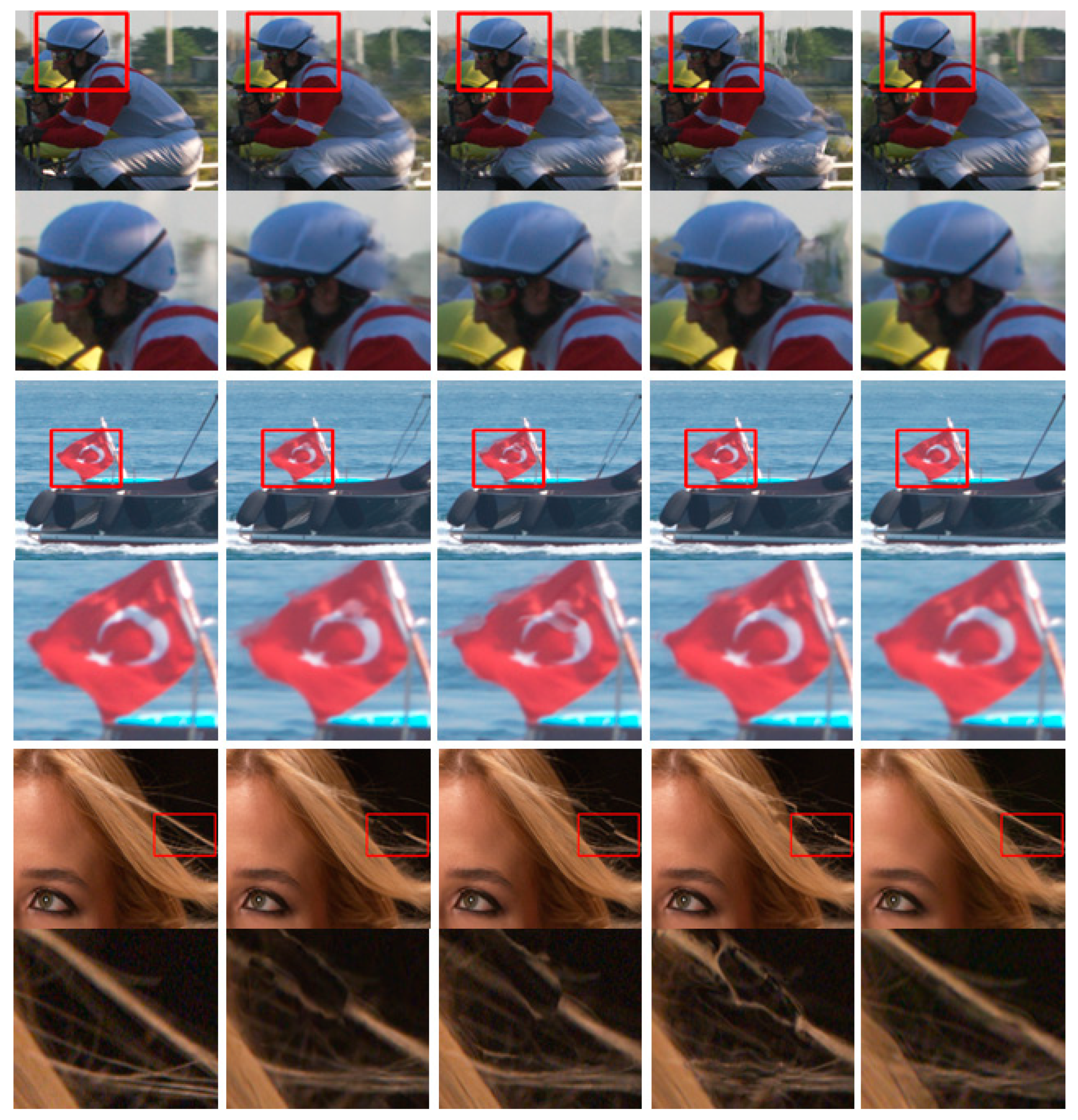
3.3. Visual Comparison

In this section, we visually compare the proposed method with the state-of-the-art methods for challenging cases for frame interpolation.

The top row of Figure 4 shows that the predicted frame of each method for a region has heavy motion, while most of the top left shows the ground-truth. Both results of SepConv are blurry, since their method cannot handle heavy motion beyond the kernel size. SuperSloMo also cannot handle this problem, and yields a blurry result. The second comparison sample is an example of complex structural changes. In the sample, the flag shakes and makes complex structural changes as the boat is sailing on a fluctuating wave. The proposed method handles this problem better than other methods and produces a good result. The final sample is fluttering hair, which makes optical flow estimation often fail. SuperSloMo, which is a flow-based method, as well as SepConv, show poor results. The proposed method shows a better result compared to the existing methods, which we attribute to the proposed low-resolution TI (temporal interpolation) network. This challenging problem set is weakened by downsampling so the TI network can handle the problem set better, and the SI (spatial interpolation) network can avoid such problems.

Table 9. Evaluation for visual comparison samples.

	First Sample		Second Sample		Third Sample
	PSNR	SSIM	PSNR	SSIM	PSNR	SSIM
SepConv-l1	22.22	0.826	29.83	0.929	20.06	0.470
SepConv-lf	22.50	0.825	28.24	0.913	19.65	0.402
SuperSloMo	20.61	0.798	31.57	0.936	20.21	0.417
Ours	24.21	0.854	31.80	0.945	21.74	0.468

shows the quantitative evaluation results for the visual comparison samples. The proposed method outperformed the existing methods in both PSNR and SSIM evaluation for the first and second samples. For the third sample, SepConv-l₁ showed better results in SSIM evaluation, but the performance gap was insignificant.

3.4. Ablation Study

We performed ablation studies to examine the effectiveness of the proposed method. For evaluation, we calculated the mean values for the PSNR and SSIM of each YCbCr channel. We first trained our network without edge loss and compared the model accuracy with the full model that utilizes every method we proposed in this paper. The network trained without edge loss performed superiorly to the full model in quantitative evaluation. However, in terms of the perceptual quality of interpolated frames, the full model produced better results, as shown in Figure 5.

We also examined the effectiveness of the proposed SI network to see how the proposed hybrid network produces better results than a method that performs temporal and spatial interpolation separately. Instead of reconstructing the Y channel of the temporally interpolated frame via our SI network, we performed spatial interpolation using the existing spatial interpolation method. For the existing spatial interpolation network, we chose VDSR [18], which has state-of-the-art performance and a comparably shallow network depth layer compared with the proposed SI network. We also trained the SI network separately, without the TI network, and performed the identical experiments.

Table 10. Effectiveness of edge loss, SI network and $I_{Y\_0}$ and $I_{Y\_2}$.

	Ultra Video		SJTU 4K Video
	PSNR	SSIM	PSNR	SSIM
Without edge loss	37.98	0.919	41.76	0.956
TI + ${\mathrm{SI}}^{\prime }$ *	36.51	0.856	39.47	0.883
TI + VDSR [18]	35.27	0.850	38.44	0.878
Without $I_{Y\_0}$ and $I_{Y\_2}$	36.05	0.862	39.82	0.898
Full model	37.02	0.917	40.55	0.950

(* ${\mathrm{SI}}^{\prime }$ denotes the SI network that trained separately without the TI network).

clearly proves that the proposed method benefits from using our SI network. Finally, we report the contribution of using $I_{Y\_0}$ and $I_{Y\_2}$ frames for the SI network. Adding these two original frames to the input of the SI network significantly increases the quantitative accuracy.

4. Conclusions

In this paper, we propose a hybrid task-based convolutional neural network for 4K video frame interpolation. We first interpolate the intermediate frame in low-resolution, then reconstruct a high-resolution frame in a coarse-to-fine fashion. In the proposed method, temporal and spatial interpolation networks, whose objectives are different, are combined into a single network in order to improve performance. Ablation studies explicitly demonstrate the advantage of using our temporal interpolation and spatial interpolation networks. The proposed method outperforms existing state-of-the-art methods in challenging cases, such as heavy motion and complex structural change. The proposed method achieved state-of-the-art performance in terms of PSNR and SSIM, as well as inference time. Experimental results show that the proposed method enables frame interpolation for 4K video and performs up to 2.69x faster than existing methods that are operable for 4K videos, while maintaining comparable visual and quantitative quality. Our work is applicable for any front-end video processing systems that handle high-resolution videos or demand fast inference time, such as set-tops or video streaming services. In future work, we plan to study the applicability of transferring learning to the interpolation of super-high-resolution video, such as 8K images. Investigating the feasibility of transferring features from different tasks such as video prediction or pixel segmentation will be the main subject of our future research.

References

1. Werlberger, M.; Pock, T.; Unger, M.; Bischof, H. Optical flow guided TV-L 1 video interpolation and restoration. In International Workshop on Energy Minimization Methods in Computer Vision and Pattern Recognition; Springer: Berlin/Heidelberg, Germany, 2011; pp. 273–286. [Google Scholar]
2. Yu, Z.; Li, H.; Wang, Z.; Hu, Z.; Chen, C.W. Multi-level video frame interpolation: Exploiting the interaction among different levels. IEEE Trans. Circuits Syst. Video Technol. 2013, 23, 1235–1248. [Google Scholar] [CrossRef]
3. Brox, T.; Bruhn, A.; Papenberg, N.; Weickert, J. High accuracy optical flow estimation based on a theory for warping. In European Conference on Computer Vision; Springer: Berlin/Heidelberg, Germany, 2004; pp. 25–36. [Google Scholar]
4. Dosovitskiy, A.; Fischer, P.; Ilg, E.; Hausser, P.; Hazirbas, C.; Golkov, V.; Van Der Smagt, P.; Cremers, D.; Brox, T. Flownet: Learning optical flow with convolutional networks. In Proceedings of the IEEE International Conference on Computer Vision, Santiago, Chile, 7–13 December 2015; pp. 2758–2766. [Google Scholar]
5. Ilg, E.; Mayer, N.; Saikia, T.; Keuper, M.; Dosovitskiy, A.; Brox, T. Flownet 2.0: Evolution of optical flow estimation with deep networks. In Proceedings of the IEEE Conference on Computer Vision and Pattern Recognition, Honolulu, HI, USA, 21–26 July 2017; pp. 2462–2470. [Google Scholar]
6. Ranjan, A.; Black, M.J. Optical flow estimation using a spatial pyramid network. In Proceedings of the IEEE Conference on Computer Vision and Pattern Recognition, Honolulu, HI, USA, 21–26 July 2017; pp. 4161–4170. [Google Scholar]
7. Ren, Z.; Yan, J.; Ni, B.; Liu, B.; Yang, X.; Zha, H. Unsupervised deep learning for optical flow estimation. In Proceedings of the Thirty-First AAAI Conference on Artificial Intelligence, San Francisco, CA, USA, 12 February 2017. [Google Scholar]
8. Sun, D.; Yang, X.; Liu, M.Y.; Kautz, J. Pwc-net: Cnns for optical flow using pyramid, warping, and cost volume. In Proceedings of the IEEE Conference on Computer Vision and Pattern Recognition, Salt Lake City, UT, USA, 18–22 June 2018; pp. 8934–8943. [Google Scholar]
9. Long, G.; Kneip, L.; Alvarez, J.M.; Li, H.; Zhang, X.; Yu, Q. Learning image matching by simply watching video. In European Conference on Computer Vision; Springer: Cham, Switzerland, 2016; pp. 434–450. [Google Scholar]
10. Liu, Z.; Yeh, R.A.; Tang, X.; Liu, Y.; Agarwala, A. Video frame synthesis using deep voxel flow. In Proceedings of the IEEE International Conference on Computer Vision, Venice, Italy, 22–29 October 2017; pp. 4463–4471. [Google Scholar]
11. Jiang, H.; Sun, D.; Jampani, V.; Yang, M.H.; Learned-Miller, E.; Kautz, J. Super slomo: High quality estimation of multiple intermediate frames for video interpolation. In Proceedings of the IEEE Conference on Computer Vision and Pattern Recognition, Salt Lake City, UT, USA, 18–22 June 2018; pp. 9000–9008. [Google Scholar]
12. Liu, Y.L.; Liao, Y.T.; Lin, Y.Y.; Chuang, Y.Y. Deep Video Frame Interpolation using Cyclic Frame Generation. In Proceedings of the AAAI Conference on Artificial Intelligence, Honolulu, HI, USA, 27 January–1 February 2019. [Google Scholar]
13. Niklaus, S.; Mai, L.; Liu, F. Video frame interpolation via adaptive convolution. In Proceedings of the IEEE Conference on Computer Vision and Pattern Recognition, Honolulu, HI, USA, 21–26 July 2017; pp. 670–679. [Google Scholar]
14. Niklaus, S.; Mai, L.; Liu, F. Video frame interpolation via adaptive separable convolution. In Proceedings of the IEEE International Conference on Computer Vision, Venice, Italy, 22–29 October 2017; pp. 261–270. [Google Scholar]
15. Niklaus, S.; Liu, F. Context-aware synthesis for video frame interpolation. In Proceedings of the IEEE Conference on Computer Vision and Pattern Recognition, Salt Lake City, UT, USA, 18–22 June 2018; pp. 1701–1710. [Google Scholar]
16. Meyer, S.; Wang, O.; Zimmer, H.; Grosse, M.; Sorkine-Hornung, A. Phase-based frame interpolation for video. In Proceedings of the IEEE Conference on Computer Vision and Pattern Recognition, Boston, MA, USA, 7–12 June 2015; pp. 1410–1418. [Google Scholar]
17. Mathieu, M.; Couprie, C.; LeCun, Y. Deep multi-scale video prediction beyond mean square error. arXiv 2015, arXiv:1511.05440. [Google Scholar]
18. Kim, J.; Kwon Lee, J.; Mu Lee, K. Accurate image super-resolution using very deep convolutional networks. In Proceedings of the IEEE Conference on Computer Vision and Pattern Recognition, Las Vegas, NV, USA, 1 July 2016; pp. 1646–1654. [Google Scholar]
19. Dong, C.; Loy, C.C.; He, K.; Tang, X. Learning a deep convolutional network for image super-resolution. In European Conference on Computer Vision; Springer: Cham, Switzerland, 2014; pp. 184–199. [Google Scholar]
20. Lim, B.; Son, S.; Kim, H.; Nah, S.; Mu Lee, K. Enhanced deep residual networks for single image super-resolution. In Proceedings of the IEEE Conference on Computer Vision and Pattern Recognition Workshops, Honolulu, HI, USA, 21–26 July 2017; pp. 136–144. [Google Scholar]
21. Lai, W.S.; Huang, J.B.; Ahuja, N.; Yang, M.H. Deep laplacian pyramid networks for fast and accurate super-resolution. In Proceedings of the IEEE Conference on Computer Vision and Pattern Recognition, Honolulu, HI, USA, 21–26 July 2017; pp. 624–632. [Google Scholar]
22. He, K.; Zhang, X.; Ren, S.; Sun, J. Deep residual learning for image recognition. In Proceedings of the IEEE Conference on Computer Vision and Pattern Recognition, Las Vegas, NV, USA, 27–30 June 2016; pp. 770–778. [Google Scholar]
23. Clevert, D.A.; Unterthiner, T.; Hochreiter, S. Fast and accurate deep network learning by exponential linear units (elus). arXiv 2015, arXiv:1511.07289. [Google Scholar]
24. Nair, V.; Hinton, G.E. Rectified linear units improve restricted boltzmann machines. In Proceedings of the 27th International Conference on Machine Learning (ICML-10), Haifa, Israel, 21–24 July 2010; pp. 807–814. [Google Scholar]
25. Ronneberger, O.; Fischer, P.; Brox, T. U-net: Convolutional networks for biomedical image segmentation. In International Conference on Medical Image Computing and Computer-Assisted Intervention; Springer: Cham, Switzerland, 2015; pp. 234–241. [Google Scholar]
26. Simonyan, K.; Zisserman, A. Very deep convolutional networks for large-scale image recognition. arXiv 2014, arXiv:1409.1556. [Google Scholar]
27. Liao, R.; Tao, X.; Li, R.; Ma, Z.; Jia, J. Video super-resolution via deep draft-ensemble learning. In Proceedings of the IEEE International Conference on Computer Vision, Araucano Park, Las Condes, Chile, 11–18 December 2015; pp. 531–539. [Google Scholar]
28. Caballero, J.; Ledig, C.; Aitken, A.; Acosta, A.; Totz, J.; Wang, Z.; Shi, W. Real-time video super-resolution with spatio-temporal networks and motion compensation. In Proceedings of the IEEE Conference on Computer Vision and Pattern Recognition, Honolulu, HI, USA, 21–26 July 2017; pp. 4778–4787. [Google Scholar]
29. Johnson, J.; Alahi, A.; Fei-Fei, L. Perceptual losses for real-time style transfer and super-resolution. In European Conference on Computer Vision; Springer: Cham, Switzerland, 2016; pp. 694–711. [Google Scholar]
30. Deng, J.; Dong, W.; Socher, R.; Li, L.J.; Li, K.; Fei-Fei, L. Imagenet: A large-scale hierarchical image database. In Proceedings of the IEEE Conference on Computer Vision and Pattern Recognition, Miami, FL, USA, 20–25 June 2009; pp. 248–255. [Google Scholar]
31. Canny, J. A computational approach to edge detection. In Readings in Computer Vision; Morgan Kaufmann: Burlington, MA, USA, 1987; pp. 184–203. [Google Scholar]
32. Xie, S.; Tu, Z. Holistically-nested edge detection. In Proceedings of the IEEE International Conference on Computer Vision, Santiago, Chile, 7–13 December 2015; pp. 1395–1403. [Google Scholar]
33. Kingma, D.P.; Ba, J. Adam: A method for stochastic optimization. arXiv 2014, arXiv:1412.6980. [Google Scholar]
34. Tao, M.; Bai, J.; Kohli, P.; Paris, S. Simple Flow: A Non-iterative, Sublinear Optical Flow Algorithm. In Computer Graphics Forum; Blackwell Publishing Ltd.: Oxford, UK, 2012; pp. 345–353. [Google Scholar]
35. Baker, S.; Scharstein, D.; Lewis, J.P.; Roth, S.; Black, M.J.; Szeliski, R. A database and evaluation methodology for optical flow. Int. J. Comput. Vis. 2011, 92, 1–31. [Google Scholar] [CrossRef]
36. Le Feuvre, J.; Thiesse, J.M.; Parmentier, M.; Raulet, M.; Daguet, C. Ultra high definition HEVC DASH data set. In Proceedings of the 5th ACM Multimedia Systems Conference, Singapore, 19 March 2014; ACM: New York, NY, USA, 2014; pp. 7–12. [Google Scholar]
37. Song, L.; Tang, X.; Zhang, W.; Yang, X.; Xia, P. The SJTU 4K video sequence dataset. In Proceedings of the IEEE 2013 Fifth International Workshop on Quality of Multimedia Experience (QoMEX), Klagenfurt am Wörthersee, Austria, 3 July 2013; pp. 34–35. [Google Scholar]
38. Wang, Z.; Bovik, A.C.; Sheikh, H.R.; Simoncelli, E.P. Image quality assessment: From error visibility to structural similarity. IEEE Trans. Image Process. 2004, 13, 600–612. [Google Scholar] [CrossRef] [PubMed]
Figure 1. The proposed method performs faster than the existing state-of-the-art methods while maintaining comparable accuracy.
Symmetry 11 00619 g001
Figure 2. Proposed video frame interpolation network architecture.
Symmetry 11 00619 g002
Figure 3. Snapshot of the evaluation dataset: (a) Ultra Video and (b) SJTU 4K Video.
Symmetry 11 00619 g003aSymmetry 11 00619 g003b
Figure 4. Visual comparison among frame interpolation methods. (From left to right: ground-truth; SepConv-l1; SepConv-lf; SuperSloMo; and Ours).
Symmetry 11 00619 g004
Figure 5. Example of the effectiveness of edge loss. (From left to right: ground-truth; without edge loss; with edge loss).
Symmetry 11 00619 g005