Univariate and Bivariate Models Related to the Generalized Epsilon–Skew–Cauchy Distribution

Abstract

In this paper, we consider a stochastic representation of the epsilon–skew–Cauchy distribution, viewed as a member of the family of skewed distributions discussed in Arellano-Valle et al. (2005). The stochastic representation facilitates derivation of distributional properties of the model. In addition, we introduce symmetric and asymmetric extensions of the Cauchy distribution, together with an extension of the epsilon–skew–Cauchy distribution. Multivariate versions of these distributions can be envisioned. Bivariate examples are discussed in some detail.

1. Introduction

Mudholkar and Hutson (2000) [1] studied an asymmetric normal distribution that they called the epsilon–skew–normal $\{ESN\left(\epsilon \right);\left|\epsilon \right|<1\}$, with asymmetry or skewness parameter $\epsilon .$ When the parameter $\epsilon$ assumes the value 0, the distribution simplifies to become a standard normal distribution. The family thus consists of a parameterized set of usually asymmetric distributions that includes the symmetric standard normal density as a special case. Specifically, we say that $X\sim ESN\left(\epsilon \right)$ if its density is of the form:

$$g\left(x;\epsilon \right)=\varphi \left(\frac{x}{1-sgn\left(x\right)\epsilon }\right)$$

where $x\in \mathbb{R}$, $\varphi$ is the standard normal density and $sgn(·)$ is the sign function.

Arellano-Valle et al. (2005) [2] discuss extension of this model, together with associated inference procedures. They consider a class of Epsilon-skew-symmetric distributions associated with a particular symmetric density $f\left(·\right)$ that is indexed by an asymmetry parameter $\epsilon$ with densities given by

$$h(x;\epsilon )=f\left(\frac{x}{1-sgn\left(x\right)\epsilon }\right)$$

(1)

where $x\in \mathbb{R}$ and $\left|\epsilon \right|<1$.

If X has density of the form (1), then we say that X is an epsilon-skew-symmetric random variable and we write $X\sim ESf\left(\epsilon \right)$. Arellano-Valle et al. (2005) [2] extend this family to the model epsilon-skew-exponential-power, a model that has major and minor asymmetry and kurtosis that the ESN model. On the other hand Gómez et al. (2007) [3] study the Fisher information matrix for epsilon-skew-t model, which was used before in the study a financial series by Hansen (1994) [4]; see also Gómez et al. (2008) [5]. Note that if in (1) we set $f\left(t\right)=1/\left(\pi \left(1+t^2\right)\right)$, we obtain the epsilon–skew–Cauchy model.

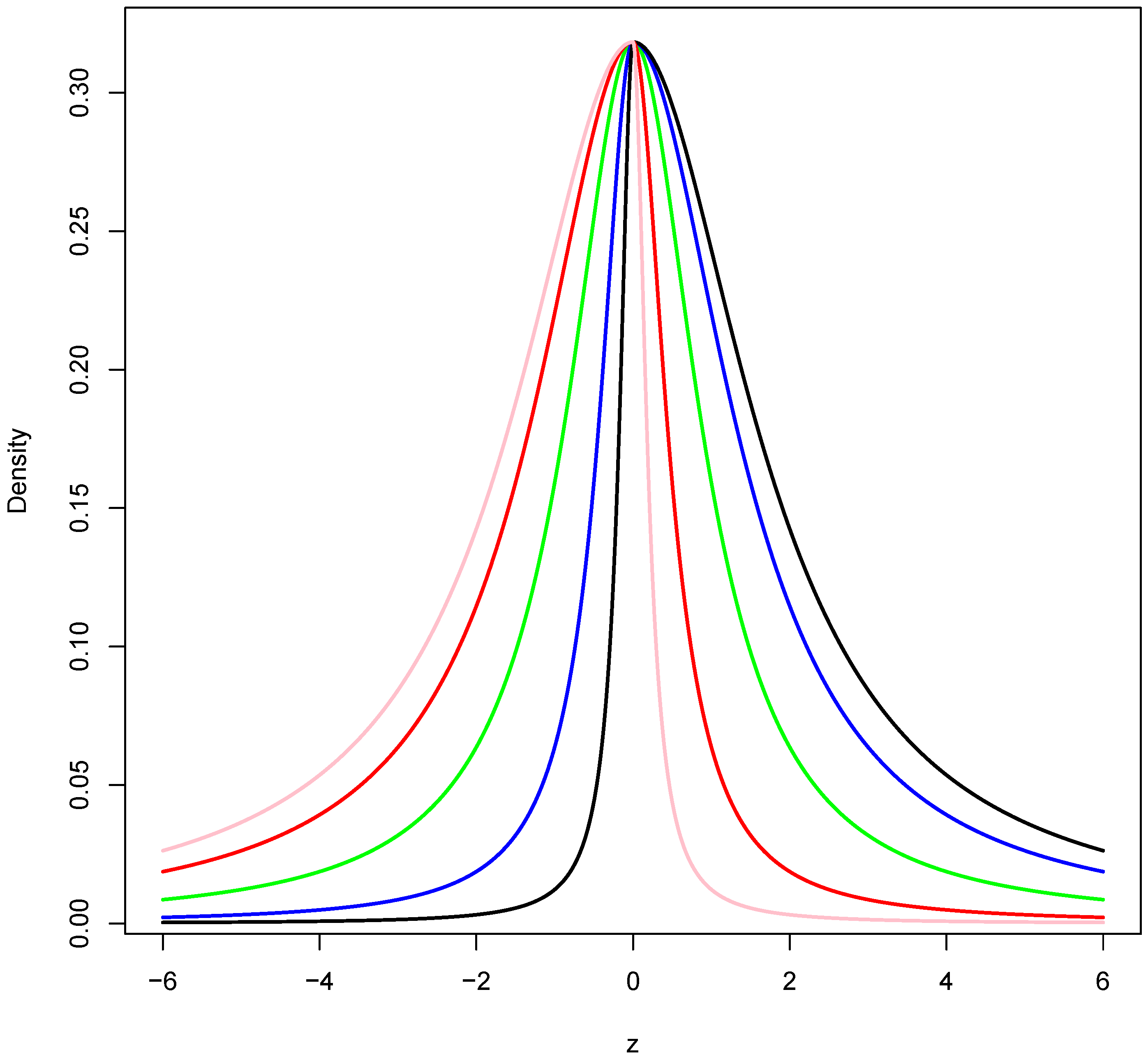
We will write $X\sim N(0,1)$ to indicate that X has a standard normal distribution, and we will write $Y\sim HN(0,1)$ to indicate that Y has a standard half-normal distribution, i.e., that $Y=\left|X\right|$ where $X\sim N(0,1).$

The distribution of the ratio $X/Y$ of two random variables is of interest in problems in biological and physical sciences, econometrics, and ranking and selection. It is well known that if $X\sim N(0,1)$, $Y_1\sim N(0,1)$ and $Y_2\sim HN(0,1)$ are independent, then the random variables $X/Y_1$ and $X/Y_2$ both have Cauchy distributions; see Johnson et al. (1994, [6] Chapter 16). Behboodian, et al. (2006) [7] and Huang and Chen (2007) [8] study the distribution of such quotients when the component random variables are skew-normal (of the form studied in Azzalini (1985) [9]). The principle objective of the present paper is to study the behavior of such quotients when the component random variables have epsilon-skew-normal distributions.

The paper is organized in the following manner. In Section 2, we describe a representation of the epsilon–skew–Cauchy model. In Section 3, we consider the distribution of the ratio of two independent random variables, one of which has an $ESN\left(\epsilon \right)$ distribution and the other a standard normal distribution. In addition, an extension of the epsilon–skew–Cauchy (ESC) distribution is introduced. Bivariate versions of these distributions are discussed in Section 4. Extensions to higher dimensions can be readily envisioned, but are not discussed here. In Section 5, some of the bivariate distributions introduced in this paper are considered as possible models for a particular real-world data set.

2. Representation of the ESC (Epsilon–Skew–Cauchy) Model

Proposition 1.

If $X\sim ESN\left(\epsilon \right)$ and $Y\sim HN(0,1)$ are independent random variables, then $Z_1\stackrel{d}{=}\frac{X}{Y}$ has an epsilon–skew–Cauchy distribution with asymmetry parameter ε and density given by

$$f_{Z_1}\left(z;\epsilon \right)=\frac{1}{\pi \left[1+{\left(\frac{z}{1-sgn\left(z\right)\epsilon }\right)}^2\right]},$$

where $z\in \mathbb{R}$, $\left|\epsilon \right|<1$ and we write $Z_1\sim ESC\left(\epsilon \right)$.

Proof. 

With the transformation $Z_1=X/Y$ and $W=Y$, whose Jacobian $\left|J\right|=w$, we obtain

$$f_{Z_1,W}\left(z,w\right)=\frac{w}{\pi }exp\left\{-\frac{1}{2}\left[\frac{z^2}{{\left(1-sgn\left(z\right)\epsilon \right)}^2}+1\right]w^2\right\},$$

where $z\in \mathbb{R},w>0$.

It follows directly that

$$f_{Z_1}\left(z;\epsilon \right)={\int }_0^{\infty }{f}_{Z_1,W}\left(z,w\right)\mathrm{d}w=\frac{1}{\pi \left[1+{\left(\frac{z}{1-sgn\left(z\right)\epsilon }\right)}^2\right]}.$$

 ☐

Figure 1 depicts the behavior of the ESC density for a variety of parameter values.

3. Generalized Cauchy Distribution

Proposition 2.

If $X\sim ESN\left({\epsilon }_1\right)$ and $Y\sim ESN\left({\epsilon }_2\right)$ are independent random variables, then $Z\stackrel{d}{=}\frac{X}{Y}$ has what we call a generalized epsilon–skew–Cauchy (GESC) distribution with parameters ${\epsilon }_1$ and ${\epsilon }_2$ and with density given by

$$f_Z\left(z;{\epsilon }_1,{\epsilon }_2\right)=\frac{1}{2\pi \left[{\left(\frac{1}{1+{\epsilon }_2}\right)}^2+{\left(\frac{z}{1+sgn\left(z\right){\epsilon }_1}\right)}^2\right]}+\frac{1}{2\pi \left[{\left(\frac{1}{1-{\epsilon }_2}\right)}^2+{\left(\frac{z}{1-sgn\left(z\right){\epsilon }_1}\right)}^2\right]},$$

where $z\in \mathbb{R}$, $|{\epsilon }_1|<1$, $|{\epsilon }_2|<1$ and we write $Z\sim GESC({\epsilon }_1,{\epsilon }_2)$.

Proof. 

Arguing as in Proposition 1, we have that

$$f_Z\left(z;{\epsilon }_1,{\epsilon }_2\right)={\int }_{-\infty }^{\infty }\frac{\left|w\right|}{2\pi }exp\left\{-\frac{1}{2}\left[\frac{z^2}{{\left(1-sgn\left(zw\right){\epsilon }_1\right)}^2}+\frac{1}{{\left(1-sgn\left(w\right){\epsilon }_2\right)}^2}\right]w^2\right\}\mathrm{d}w.$$

By considering separately the cases in which $z\ge 0$ and $z<0$, result follows directly. ☐

From Proposition 2 two special cases are obtained directly,

• If ${\epsilon }_2=0$ a generalized Cauchy (GC) distribution is obtained. In this case we write $Z\sim GC\left(\epsilon \right)$, and its pdf is given by

  $$f_Z\left(z;\epsilon \right)=\frac{1}{2\pi \left[1+{\left(\frac{z}{1+sgn\left(z\right)\epsilon }\right)}^2\right]}+\frac{1}{2\pi \left[1+{\left(\frac{z}{1-sgn\left(z\right)\epsilon }\right)}^2\right]},$$

  where $z\in \mathbb{R}$, $0<\epsilon <1$ and $Z\stackrel{d}{=}X/Y$ where $X\sim ESN\left(\epsilon \right)$ and $Y\sim N(0,1)$ are independent random variables.
• If ${\epsilon }_1={\epsilon }_2=\epsilon$ an epsilon–skew–Cauchy distribution is obtained. In this case we write $Z\sim ESC2\left(\epsilon \right)$, and its pdf is given by

  $$f_Z\left(z;\epsilon \right)=\frac{1}{2\pi \left[{\left(\frac{1}{1+\epsilon }\right)}^2+{\left(\frac{z}{1+sgn\left(z\right)\epsilon }\right)}^2\right]}+\frac{1}{2\pi \left[{\left(\frac{1}{1-\epsilon }\right)}^2+{\left(\frac{z}{1-sgn\left(z\right)\epsilon }\right)}^2\right]},$$

  where $z\in \mathbb{R}$, $\left|\epsilon \right|<1$ and $Z\stackrel{d}{=}X/Y$ where $X\sim ESN\left(\epsilon \right)$ and $Y\sim ESN\left(\epsilon \right)$ are independent random variables.

4. General Bivariate Mudholkar-Hutson Distribution

Define $Z_1,Z_2,Z_3$ to be i.i.d. standard normal random variables. For $i=1,2,3$ define

$$U_i=\left\{\begin{array}{cc}-{\alpha }_i& \mathrm{with}\mathrm{probability}{\gamma }_i\\ {\beta }_i& \mathrm{with}\mathrm{probability}1-{\gamma }_i\end{array}\right.$$

where ${\alpha }_1$, ${\alpha }_2$, ${\alpha }_3$, ${\beta }_1$, ${\beta }_2$, ${\beta }_3$ are positive numbers and $0<{\gamma }_1,{\gamma }_2,{\gamma }_3<1$. So, the parameters ${\alpha }_i$ and ${\beta }_i$ indicate the propensity in which the discrete random variable takes negative and positive values, respectively. The parameters ${\gamma }_i$ control how often negative and positive values are taken by $U_i$.

In addition assume that all six random variables $Z_1,Z_2,Z_3,U_1,U_2$ and $U_3$ are independent, and define

$$(X,Y)=\left(\frac{U_1\left|Z_1\right|}{U_3\left|Z_3\right|},\frac{U_2\left|Z_2\right|}{U_3\left|Z_3\right|}\right).$$

(2)

The model (2) is highly flexible since it allows for different behavior in each of the four quadrants of the plane. From (2) it may be recognized that only fractional moments of X and Y exist.

Note that if we define $\left(W_1,W_2\right)=\left(\frac{\left|Z_1\right|}{\left|Z_3\right|},\frac{\left|Z_2\right|}{\left|Z_3\right|}\right)$, it is readily verified that

$$f_{W_1,W_2}\left(w_1,w_2\right)=\frac{2}{\pi }{\left(1+w_1^2+w_2^2\right)}^{-3/2}I\left(w_1>0,w_2>0\right),$$

(3)

in which case we say that $\left(W_1,W_2\right)$ has a standard bivariate half-Cauchy distribution.

Using (3) and conditioning on $U_1,U_2$ and $U_3$ we obtain the density of $(X,Y)$ in the albeit complicated form:

$$\begin{array}{ccc}f(x,y)& =& \frac{2}{\pi }\left\{{\gamma }_1{\gamma }_2{\gamma }_3\frac{{\alpha }_3^2}{{\alpha }_1{\alpha }_2}{\left[1+{\left(\frac{{\alpha }_3}{{\alpha }_1}x\right)}^2+{\left(\frac{{\alpha }_3}{{\alpha }_2}y\right)}^2\right]}^{-3/2}I(x>0,y>0)\right\}\hfill \\ & & +\frac{2}{\pi }\left\{{\gamma }_1{\gamma }_2(1-{\gamma }_3)\frac{{\beta }_3^2}{{\alpha }_1{\alpha }_2}{\left[1+{\left(\frac{{\beta }_3}{{\alpha }_1}x\right)}^2+{\left(\frac{{\beta }_3}{{\alpha }_2}y\right)}^2\right]}^{-3/2}I(x<0,y<0)\right\}\hfill \\ & & +\frac{2}{\pi }\left\{{\gamma }_1(1-{\gamma }_2){\gamma }_3\frac{{\alpha }_3^2}{{\alpha }_1{\beta }_2}{\left[1+{\left(\frac{{\alpha }_3}{{\alpha }_1}x\right)}^2+{\left(\frac{{\alpha }_3}{{\beta }_2}y\right)}^2\right]}^{-3/2}I(x>0,y<0)\right\}\hfill \\ & & +\frac{2}{\pi }\left\{{\gamma }_1(1-{\gamma }_2)(1-{\gamma }_3)\frac{{\beta }_3^2}{{\alpha }_1{\beta }_2}{\left[1+{\left(\frac{{\beta }_3}{{\alpha }_1}x\right)}^2+{\left(\frac{{\beta }_3}{{\beta }_2}y\right)}^2\right]}^{-3/2}I(x<0,y>0)\right\}\hfill \\ & & +\frac{2}{\pi }\left\{(1-{\gamma }_1){\gamma }_2{\gamma }_3\frac{{\alpha }_3^2}{{\beta }_1{\alpha }_2}{\left[1+{\left(\frac{{\alpha }_3}{{\beta }_1}x\right)}^2+{\left(\frac{{\alpha }_3}{{\alpha }_2}y\right)}^2\right]}^{-3/2}I(x<0,y>0)\right\}\hfill \\ & & +\frac{2}{\pi }\left\{(1-{\gamma }_1){\gamma }_2(1-{\gamma }_3)\frac{{\beta }_3^2}{{\beta }_1{\alpha }_2}{\left[1+{\left(\frac{{\beta }_3}{{\beta }_1}x\right)}^2+{\left(\frac{{\beta }_3}{{\alpha }_2}y\right)}^2\right]}^{-3/2}I(x>0,y<0)\right\}\hfill \\ & & +\frac{2}{\pi }\left\{(1-{\gamma }_1)(1-{\gamma }_2){\gamma }_3\frac{{\alpha }_3^2}{{\beta }_1{\beta }_2}{\left[1+{\left(\frac{{\alpha }_3}{{\beta }_1}x\right)}^2+{\left(\frac{{\alpha }_3}{{\beta }_2}y\right)}^2\right]}^{-3/2}I(x<0,y<0)\right\}\hfill \\ & & +\frac{2}{\pi }\left\{(1-{\gamma }_1)(1-{\gamma }_2)(1-{\gamma }_3)\frac{{\beta }_3^2}{{\beta }_1{\beta }_2}{\left[1+{\left(\frac{{\beta }_3}{{\beta }_1}x\right)}^2+{\left(\frac{{\beta }_3}{{\beta }_2}y\right)}^2\right]}^{-3/2}I(x>0,y>0)\right\}.\hfill \end{array}$$

(4)

Some special cases which might be considered include the following:

• Mudholkar and Hutson type. For this we set: ${\alpha }_i=1+{\epsilon }_i$, ${\beta }_i=1-{\epsilon }_i$ and ${\gamma }_i=\left(1+{\epsilon }_i\right)/2$ for $i=1,2,3$.
  In this case the density (4) simplifies somewhat to become:

  $$\begin{array}{ccc}f(x,y)& =& \frac{1}{4\pi }\left\{{(1+{\epsilon }_3)}^3{\left[1+{\left(\frac{1+{\epsilon }_3}{1+{\epsilon }_1}x\right)}^2+{\left(\frac{1+{\epsilon }_3}{1+{\epsilon }_2}y\right)}^2\right]}^{-3/2}I(x>0,y>0)\right\}\hfill \\ & & +\frac{1}{4\pi }\left\{{(1-{\epsilon }_3)}^3{\left[1+{\left(\frac{1-{\epsilon }_3}{1+{\epsilon }_1}x\right)}^2+{\left(\frac{1-{\epsilon }_3}{1+{\epsilon }_2}y\right)}^2\right]}^{-3/2}I(x<0,y<0)\right\}\hfill \\ & & +\frac{1}{4\pi }\left\{{(1+{\epsilon }_3)}^3{\left[1+{\left(\frac{1+{\epsilon }_3}{1+{\epsilon }_1}x\right)}^2+{\left(\frac{1+{\epsilon }_3}{1-{\epsilon }_2}y\right)}^2\right]}^{-3/2}I(x>0,y<0)\right\}\hfill \\ & & +\frac{1}{4\pi }\left\{{(1-{\epsilon }_3)}^3{\left[1+{\left(\frac{1-{\epsilon }_3}{1+{\epsilon }_1}x\right)}^2+{\left(\frac{1-{\epsilon }_3}{1-{\epsilon }_2}y\right)}^2\right]}^{-3/2}I(x<0,y>0)\right\}\hfill \\ & & +\frac{1}{4\pi }\left\{{(1+{\epsilon }_3)}^3{\left[1+{\left(\frac{1+{\epsilon }_3}{1-{\epsilon }_1}x\right)}^2+{\left(\frac{1+{\epsilon }_3}{1+{\epsilon }_2}y\right)}^2\right]}^{-3/2}I(x<0,y>0)\right\}\hfill \\ & & +\frac{1}{4\pi }\left\{{(1-{\epsilon }_3)}^3{\left[1+{\left(\frac{1-{\epsilon }_3}{1-{\epsilon }_1}x\right)}^2+{\left(\frac{1-{\epsilon }_3}{1+{\epsilon }_2}y\right)}^2\right]}^{-3/2}I(x>0,y<0)\right\}\hfill \\ & & +\frac{1}{4\pi }\left\{{(1+{\epsilon }_3)}^3{\left[1+{\left(\frac{1+{\epsilon }_3}{1-{\epsilon }_1}x\right)}^2+{\left(\frac{1+{\epsilon }_3}{1-{\epsilon }_2}y\right)}^2\right]}^{-3/2}I(x<0,y<0)\right\}\hfill \\ & & +\frac{1}{4\pi }\left\{{(1-{\epsilon }_3)}^3{\left[1+{\left(\frac{1-{\epsilon }_3}{1-{\epsilon }_1}x\right)}^2+{\left(\frac{1-{\epsilon }_3}{1-{\epsilon }_2}y\right)}^2\right]}^{-3/2}I(x>0,y>0)\right\}.\hfill \end{array}$$

  (5)
  A further specialization of the density (5) can be considered, as follows.
• Homogenous Mudholkar and Hutson type. For this we set: ${\alpha }_i=1+\epsilon$, ${\beta }_i=1-\epsilon$ and ${\gamma }_i=\left(1+\epsilon \right)/2$ for $i=1,2,3$.
  This homogeneity results in a little simplification of (4), thus:

  $$\begin{array}{ccc}f\left(x,y;\epsilon \right)& =& \frac{1}{4\pi }\left\{\left[{(1+\epsilon )}^3+{(1-\epsilon )}^3\right]{\left[1+x^2+y^2\right]}^{-3/2}I(x>0,y>0)\right\}\hfill \\ & & +\frac{1}{4\pi }\left\{{(1-\epsilon )}^3{\left[1+{\left(\frac{1-\epsilon }{1+\epsilon }x\right)}^2+{\left(\frac{1-\epsilon }{1+\epsilon }y\right)}^2\right]}^{-3/2}I(x<0,y<0)\right\}\hfill \\ & & +\frac{1}{4\pi }\left\{{(1+\epsilon )}^3{\left[1+x^2+{\left(\frac{1+\epsilon }{1-\epsilon }y\right)}^2\right]}^{-3/2}I(x>0,y<0)\right\}\hfill \\ & & +\frac{1}{4\pi }\left\{{(1-\epsilon )}^3{\left[1+{\left(\frac{1-\epsilon }{1+\epsilon }x\right)}^2+y^2\right]}^{-3/2}I(x<0,y>0)\right\}\hfill \\ & & +\frac{1}{4\pi }\left\{{(1+\epsilon )}^3{\left[1+{\left(\frac{1+\epsilon }{1-\epsilon }x\right)}^2+y^2\right]}^{-3/2}I(x<0,y>0)\right\}\hfill \\ & & +\frac{1}{4\pi }\left\{{(1-\epsilon )}^3{\left[1+x^2+{\left(\frac{1-\epsilon }{1+\epsilon }y\right)}^2\right]}^{-3/2}I(x>0,y<0)\right\}\hfill \\ & & +\frac{1}{4\pi }\left\{{(1+\epsilon )}^3{\left[1+{\left(\frac{1+\epsilon }{1-\epsilon }x\right)}^2+{\left(\frac{1+\epsilon }{1-\epsilon }y\right)}^2\right]}^{-3/2}I(x<0,y<0)\right\}.\hfill \end{array}$$

  (6)
  It is easy to see that the parameter $\epsilon$ is not identifiable in (6) because $f\left(x,y;\epsilon \right)=f\left(x,y;-\epsilon \right)$. An adjustment to ensure identifiability involves introducing the constraint $\epsilon \ge 0$.
• Equal weights. In this case we assume that ${\alpha }_1,$ ${\alpha }_2,$ ${\alpha }_3,$ ${\beta }_1,{\beta }_2,{\beta }_3$ are positive numbers and ${\gamma }_i=1/2$ for $i=1,2,3$.

  $$\begin{array}{ccc}f\left(x,y\right)& =& \frac{1}{4\pi }\left\{\frac{{\alpha }_3^2}{{\alpha }_1{\alpha }_2}{\left[1+{\left(\frac{{\alpha }_3}{{\alpha }_1}x\right)}^2+{\left(\frac{{\alpha }_3}{{\alpha }_2}y\right)}^2\right]}^{-3/2}+\frac{{\beta }_3^2}{{\beta }_1{\beta }_2}{\left[1+{\left(\frac{{\beta }_3}{{\beta }_1}x\right)}^2+{\left(\frac{{\beta }_3}{{\beta }_2}y\right)}^2\right]}^{-3/2}\right\}\hfill \\ & & \times I\left(x>0,y>0\right)\hfill \\ & & +\frac{1}{4\pi }\left\{\frac{{\beta }_3^2}{{\alpha }_1{\alpha }_2}{\left[1+{\left(\frac{{\beta }_3}{{\alpha }_1}x\right)}^2+{\left(\frac{{\beta }_3}{{\alpha }_2}y\right)}^2\right]}^{-3/2}+\frac{{\alpha }_3^2}{{\beta }_1{\beta }_2}{\left[1+{\left(\frac{{\alpha }_3}{{\beta }_1}x\right)}^2+{\left(\frac{{\alpha }_3}{{\beta }_2}y\right)}^2\right]}^{-3/2}\right\}\hfill \\ & & \times I\left(x<0,y<0\right)\hfill \\ & & +\frac{1}{4\pi }\left\{\frac{{\alpha }_3^2}{{\alpha }_1{\beta }_2}{\left[1+{\left(\frac{{\alpha }_3}{{\alpha }_1}x\right)}^2+{\left(\frac{{\alpha }_3}{{\beta }_2}y\right)}^2\right]}^{-3/2}+\frac{{\beta }_3^2}{{\beta }_1{\alpha }_2}{\left[1+{\left(\frac{{\beta }_3}{{\beta }_1}x\right)}^2+{\left(\frac{{\beta }_3}{{\alpha }_2}y\right)}^2\right]}^{-3/2}\right\}\hfill \\ & & \times I\left(x>0,y<0\right)\hfill \\ & & +\frac{1}{4\pi }\left\{\frac{{\alpha }_3^2}{{\beta }_1{\alpha }_2}{\left[1+{\left(\frac{{\alpha }_3}{{\beta }_1}x\right)}^2+{\left(\frac{{\alpha }_3}{{\alpha }_2}y\right)}^2\right]}^{-3/2}+\frac{{\beta }_3^2}{{\alpha }_1{\beta }_2}{\left[1+{\left(\frac{{\beta }_3}{{\alpha }_1}x\right)}^2+{\left(\frac{{\beta }_3}{{\beta }_2}y\right)}^2\right]}^{-3/2}\right\}\hfill \\ & & \times I\left(x<0,y>0\right).\hfill \end{array}$$

  (7)
  The pdf (7) is not identifiable because the values of ${\alpha }_i$ can be interchanged with those of ${\beta }_i$ and $f(x,y)$ does not change. Moreover, multiplying all of the $\alpha$’s and $\beta$’s by a constant does not change $f(x,y)$. So, one way to get identifiability in the model (7) is to set ${\alpha }_i={\beta }_i$ $\left(i=1,2,3\right)$ and ${\alpha }_3$ equal to 1. In that case, Equation (7) takes the form

  $$f\left(x,y\right)=\frac{1}{2\pi }\frac{1}{{\alpha }_1{\alpha }_2}{\left[1+{\left(\frac{x}{{\alpha }_1}\right)}^2+{\left(\frac{y}{{\alpha }_2}\right)}^2\right]}^{-3/2}.$$
  However, this is then recognizable as being simply a scaled version of the standard bivariate Cauchy density (compare with Equation (3)).

We now consider the marginal densities for the random variable $(X,Y)$ defined by (2). From (2) we have $X=\frac{U_1\left|Z_1\right|}{U_3\left|Z_3\right|}$ and $Y=\frac{U_2\left|Z_2\right|}{U_3\left|Z_3\right|}$ and the density of $W_1=\frac{|Z_1|}{|Z_3|}=\left|\frac{Z_1}{Z_3}\right|$ is a standard half-Cauchy density, i.e., $f_{W_1}\left(w_1\right)=\frac{2}{\pi }{(1+w_1^2)}^{-1}$.

Consequently, the density of X is of the form

$$\begin{array}{ccc}{f}_X\left(x\right)& =& \frac{2}{\pi }{\gamma }_1{\gamma }_3\frac{{\alpha }_3}{{\alpha }_1}{\left[1+{\left(\frac{{\alpha }_3}{{\alpha }_1}x\right)}^2\right]}^{-1}I\left(x>0\right)+\frac{2}{\pi }{\gamma }_1(1-{\gamma }_3)\frac{{\beta }_3}{{\alpha }_1}{\left[1+{\left(\frac{{\beta }_3}{{\alpha }_1}x\right)}^2\right]}^{-1}I\left(x<0\right)\hfill \\ & & +\frac{2}{\pi }(1-{\gamma }_1)\left\{{\gamma }_3\frac{{\alpha }_3}{{\beta }_1}{\left[1+{\left(\frac{{\alpha }_3}{{\beta }_1}x\right)}^2\right]}^{-1}I\left(x<0\right)+(1-{\gamma }_3)\frac{{\beta }_3}{{\beta }_1}{\left[1+{\left(\frac{{\beta }_3}{{\beta }_1}x\right)}^2\right]}^{-1}I\left(x>0\right)\right\},\hfill \end{array}$$

which is a mixture of half-Cauchy densities. The density of Y is then of the same form with ${\alpha }_1,{\beta }_1$ replaced by ${\alpha }_2,{\beta }_2$.

To get a more direct bivariate version of the original Mudholkar-Hutson density in which the $\alpha$’s, $\beta$’s and $\gamma$’s were related to each other, we go back to the original representation, i.e., Equation (2), but now we set ${\alpha }_1=\left(1+{\epsilon }_1\right)$, ${\beta }_1=\left(1-{\epsilon }_1\right)$, ${\gamma }_1=\left(1+{\epsilon }_1\right)/2$, ${\alpha }_2=\left(1+{\epsilon }_2\right)$, ${\beta }_2=\left(1-{\epsilon }_2\right)$, ${\gamma }_2=\left(1+{\epsilon }_2\right)/2$ and ${\alpha }_3={\beta }_3={\gamma }_3=1$. So the density is of the form

$$\begin{array}{ccc}f\left(x,y\right)\hfill & =& \frac{1}{2\pi }{\left[1+{\left(\frac{x}{1+{\epsilon }_1}\right)}^2+{\left(\frac{y}{1+{\epsilon }_2}\right)}^2\right]}^{-3/2}I\left(x>0,y>0\right)\hfill \\ & & +\frac{1}{2\pi }{\left[1+{\left(\frac{x}{1+{\epsilon }_1}\right)}^2+{\left(\frac{y}{1-{\epsilon }_2}\right)}^2\right]}^{-3/2}I\left(x>0,y<0\right)\hfill \\ & & +\frac{1}{2\pi }{\left[1+{\left(\frac{x}{1-{\epsilon }_1}\right)}^2+{\left(\frac{y}{1+{\epsilon }_2}\right)}^2\right]}^{-3/2}I\left(x<0,y>0\right)\hfill \\ & & +\frac{1}{2\pi }{\left[1+{\left(\frac{x}{1-{\epsilon }_1}\right)}^2+{\left(\frac{y}{1-{\epsilon }_2}\right)}^2\right]}^{-3/2}I\left(x<0,y<0\right)\hfill \end{array}$$

with marginal density

$$f_X\left(x\right)=\frac{1}{\pi }{\left[1+{\left(\frac{x}{1+{\epsilon }_1}\right)}^2\right]}^{-1}I\left(x>0\right)+\frac{1}{\pi }{\left[1+{\left(\frac{x}{1-{\epsilon }_1}\right)}^2\right]}^{-1}I\left(x<0\right).$$

A more general version of the density with ${\gamma }_3=1,$ is of the form: (without loss of generality set ${\alpha }_3=1$)

$$\begin{array}{ccc}f\left(x,y\right)\hfill & =& \frac{2}{\pi }\left\{{\gamma }_1{\gamma }_2\frac{1}{{\alpha }_1{\alpha }_2}{\left[1+{\left(\frac{x}{{\alpha }_1}\right)}^2+{\left(\frac{y}{{\alpha }_2}\right)}^2\right]}^{-3/2}I\left(x>0,y>0\right)\right\}\hfill \\ & & +\frac{2}{\pi }\left\{{\gamma }_1(1-{\gamma }_2)\frac{1}{{\alpha }_1{\beta }_2}{\left[1+{\left(\frac{x}{{\alpha }_1}\right)}^2+{\left(\frac{y}{{\beta }_2}\right)}^2\right]}^{-3/2}I\left(x>0,y<0\right)\right\}\hfill \\ & & +\frac{2}{\pi }\left\{(1-{\gamma }_1){\gamma }_2\frac{1}{{\beta }_1{\alpha }_2}{\left[1+{\left(\frac{x}{{\beta }_1}\right)}^2+{\left(\frac{y}{{\alpha }_2}\right)}^2\right]}^{-3/2}I\left(x<0,y>0\right)\right\}\hfill \\ & & +\frac{2}{\pi }\left\{(1-{\gamma }_1)(1-{\gamma }_2)\frac{1}{{\beta }_1{\beta }_2}{\left[1+{\left(\frac{x}{{\beta }_1}\right)}^2+{\left(\frac{y}{{\beta }_2}\right)}^2\right]}^{3/2}I\left(x<0,y<0\right)\right\}\hfill \end{array}$$

with corresponding marginal

$$f_X\left(x\right)=\frac{2}{\pi }{\gamma }_1\frac{1}{{\alpha }_1}{\left[1+{\left(\frac{x}{{\alpha }_1}\right)}^2\right]}^{-1}I\left(x>0\right)+\frac{2}{\pi }(1-{\gamma }_1)\frac{1}{{\beta }_1}{\left[1+{\left(\frac{x}{{\beta }_1}\right)}^2\right]}^{-1}I\left(x<0\right).$$

Needless to say we can consider analogous models in which, instead of assuming that $(W_1,W_2)=\left(\frac{|Z_1|}{|Z_3|},\frac{|Z_2|}{|Z_3|}\right)$ has a density of the form (3) we assume that it has another bivariate density with support ${\mathbb{R}}^{+}\times {\mathbb{R}}^{+}$, e.g., bivariate normal restricted to ${\mathbb{R}}^{+}\times {\mathbb{R}}^{+}$, or bivariate Pareto, etc.

Another general bivariate MH model which includes the bivariate skew-Cauchy distribution given by (2) is the bivariate skew t model. This model can be obtained replacing $\left|Z_3\right|$ by $V_3\sim {\chi }_{\nu }^2$ in Equation (2). Thus, if we assume that all six random variables $Z_1,Z_2\stackrel{\mathrm{iid}}{\sim }N\left(0,1\right)$, $V_3\sim {\chi }_{\nu }^2$; $U_1,U_2$ and $U_3$ are independent, and define

$$(X,Y)=\left(\frac{U_1\left|Z_1\right|}{U_3\sqrt{V_3/\nu }},\frac{U_2\left|Z_2\right|}{U_3\sqrt{V_3/\nu }}\right),$$

(8)

then, because $\left(W_1,W_2\right)=\left(\frac{\left|Z_1\right|}{\sqrt{V_3/\nu }},\frac{\left|Z_2\right|}{\sqrt{V_3/\nu }}\right)$ has density

$$f_{W_1,W_2}\left(w_1,w_2\right)=\frac{2}{\pi }{\left(1+\frac{w_1^2+w_2^2}{\nu }\right)}^{-\left(\nu +2\right)/2}I\left(w_1>0,w_2>0\right),$$

the density of $(X,Y)$ is

$$\begin{array}{ccc}f\left(x,y\right)& =& \int f\left(x,y\left|u_1,u_2,u_3\right.\right)f\left(u_1,u_2,u_3\right)\mathrm{d}{u}_1\mathrm{d}{u}_2\mathrm{d}{u}_3\hfill \\ & =& \int \frac{u_3^2}{u_1{u}_2}{f}_{W_1,W_2}\left(\left.\frac{u_3}{u_1}x,\frac{u_3}{u_2}y\right|u_1,u_2,u_3\right)f\left(u_1,u_2,u_3\right)\mathrm{d}{u}_1\mathrm{d}{u}_2\mathrm{d}{u}_3\hfill \\ & =& \int \frac{2}{\pi }\frac{u_3^2}{u_1{u}_2}{\left[1+\frac{1}{\nu }{\left(\frac{u_3}{u_1}x\right)}^2+\frac{1}{\nu }{\left(\frac{u_3}{u_2}y\right)}^2\right]}^{-\left(\nu +2\right)/2}f\left(u_1,u_2,u_3\right)\mathrm{d}{u}_1\mathrm{d}{u}_2\mathrm{d}{u}_3\hfill \\ & =& \frac{2}{\pi }\left\{{\gamma }_1{\gamma }_2{\gamma }_3\frac{{\alpha }_3^2}{{\alpha }_1{\alpha }_2}{\left[1+\frac{1}{\nu }{\left(\frac{{\alpha }_3}{{\alpha }_1}x\right)}^2+\frac{1}{\nu }{\left(\frac{{\alpha }_3}{{\alpha }_2}y\right)}^2\right]}^{-\left(\nu +2\right)/2}I(x>0,y>0)\right\}\hfill \\ & & +\frac{2}{\pi }\left\{{\gamma }_1{\gamma }_2(1-{\gamma }_3)\frac{{\beta }_3^2}{{\alpha }_1{\alpha }_2}{\left[1+\frac{1}{\nu }{\left(\frac{{\beta }_3}{{\alpha }_1}x\right)}^2+\frac{1}{\nu }{\left(\frac{{\beta }_3}{{\alpha }_2}y\right)}^2\right]}^{-\left(\nu +2\right)/2}I(x<0,y<0)\right\}\hfill \\ & & +\frac{2}{\pi }\left\{{\gamma }_1(1-{\gamma }_2){\gamma }_3\frac{{\alpha }_3^2}{{\alpha }_1{\beta }_2}{\left[1+\frac{1}{\nu }{\left(\frac{{\alpha }_3}{{\alpha }_1}x\right)}^2+\frac{1}{\nu }{\left(\frac{{\alpha }_3}{{\beta }_2}y\right)}^2\right]}^{-\left(\nu +2\right)/2}I(x>0,y<0)\right\}\hfill \\ & & +\frac{2}{\pi }\left\{{\gamma }_1(1-{\gamma }_2)(1-{\gamma }_3)\frac{{\beta }_3^2}{{\alpha }_1{\beta }_2}{\left[1+\frac{1}{\nu }{\left(\frac{{\beta }_3}{{\alpha }_1}x\right)}^2+\frac{1}{\nu }{\left(\frac{{\beta }_3}{{\beta }_2}y\right)}^2\right]}^{-\left(\nu +2\right)/2}I(x<0,y>0)\right\}\hfill \\ & & +\frac{2}{\pi }\left\{(1-{\gamma }_1){\gamma }_2{\gamma }_3\frac{{\alpha }_3^2}{{\beta }_1{\alpha }_2}{\left[1+\frac{1}{\nu }{\left(\frac{{\alpha }_3}{{\beta }_1}x\right)}^2+\frac{1}{\nu }{\left(\frac{{\alpha }_3}{{\alpha }_2}y\right)}^2\right]}^{-\left(\nu +2\right)/2}I(x<0,y>0)\right\}\hfill \\ & & +\frac{2}{\pi }\left\{(1-{\gamma }_1){\gamma }_2(1-{\gamma }_3)\frac{{\beta }_3^2}{{\beta }_1{\alpha }_2}{\left[1+\frac{1}{\nu }{\left(\frac{{\beta }_3}{{\beta }_1}x\right)}^2+\frac{1}{\nu }{\left(\frac{{\beta }_3}{{\alpha }_2}y\right)}^2\right]}^{-\left(\nu +2\right)/2}I(x>0,y<0)\right\}\hfill \\ & & +\frac{2}{\pi }\left\{(1-{\gamma }_1)(1-{\gamma }_2){\gamma }_3\frac{{\alpha }_3^2}{{\beta }_1{\beta }_2}{\left[1+\frac{1}{\nu }{\left(\frac{{\alpha }_3}{{\beta }_1}x\right)}^2+\frac{1}{\nu }{\left(\frac{{\alpha }_3}{{\beta }_2}y\right)}^2\right]}^{-\left(\nu +2\right)/2}I(x<0,y<0)\right\}\hfill \\ & & +\frac{2}{\pi }\left\{(1-{\gamma }_1)(1-{\gamma }_2)(1-{\gamma }_3)\frac{{\beta }_3^2}{{\beta }_1{\beta }_2}{\left[1+\frac{1}{\nu }{\left(\frac{{\beta }_3}{{\beta }_1}x\right)}^2+\frac{1}{\nu }{\left(\frac{{\beta }_3}{{\beta }_2}y\right)}^2\right]}^{-\left(\nu +2\right)/2}I(x>0,y>0)\right\}.\hfill \end{array}$$

(9)

The pair of variables in (8) allows one to model a wider variety of paired data sets than that given in (2) because it also can model light and heavy “tails” in a different way for each quadrant of the coordinate axis. Additionally, it is possible to compute the $r-$order moments.

Proposition 3.

The expected value of $(X,Y)$ in (8) is given by

$$\mathbb{E}\left(X,Y\right)=\frac{\sqrt{\nu }}{\sqrt{\pi }}\left({\beta }_1\left(1-{\gamma }_1\right)-{\alpha }_1{\gamma }_1,{\beta }_2\left(1-{\gamma }_2\right)-{\alpha }_2{\gamma }_2\right)\left(\frac{1-{\gamma }_3}{{\beta }_3}-\frac{{\gamma }_3}{{\alpha }_3}\right)\frac{\mathsf{\Gamma }\left(\nu /2-1/2\right)}{\mathsf{\Gamma }\left(\nu /2\right)},$$

provided that $\nu >1$.

Proof. 

For $i=1,2$ it is immediate that $\mathbb{E}\left(U_i\right)\mathbb{E}\left(\left|Z_i\right|\right)=\left({\beta }_i\left(1-{\gamma }_i\right)-{\alpha }_i{\gamma }_i\right)\sqrt{2}/\sqrt{\pi }$ and $\mathbb{E}\left(U_3^{-1}\right)=\left(1-{\gamma }_3\right)/{\beta }_3-{\gamma }_3/{\alpha }_3$.

On the other hand, since $V_3\sim {\chi }_{\nu }^2$ then

$$\mathbb{E}\left(\frac{\sqrt{\nu }}{\sqrt{V_3}}\right)={\int }_0^{\infty }\frac{\sqrt{\nu }}{\sqrt{x}}\frac{x^{\nu /2-1}}{2^{\nu /2}\mathsf{\Gamma }\left(\nu /2\right)}{e}^{-x/2}\mathrm{d}x\stackrel{\nu >1}{=}\frac{\sqrt{\nu }\mathsf{\Gamma }\left(\nu /2-1/2\right)}{\sqrt{2}\mathsf{\Gamma }\left(\nu /2\right)}.$$

Therefore, from (8) we have

$$\mathbb{E}\left(X,Y\right)=\left(\mathbb{E}\left(U_1\right)\mathbb{E}\left(\left|Z_1\right|\right),\mathbb{E}\left(U_2\right)\mathbb{E}\left(\left|Z_2\right|\right)\right)\mathbb{E}\left(\frac{1}{U_3}\right)\mathbb{E}\left(\frac{\sqrt{\nu }}{\sqrt{V_3}}\right)$$

and the result is obtained straightforward. ☐

Following the proof of the previous proposition it is possible to obtain the $r-$order moments provided that $\nu >r$.

In applications, it will usually be appropriate to augment these models by the introduction of location, scale and rotation parameters, i.e., to consider

$$\left(\tilde{X},\tilde{Y}\right)=\mathbf{\mu }+{\mathbf{\Sigma }}^{1/2}\left(X,Y\right),$$

where $\underline{\mu }\in {\left(-\infty ,\infty \right)}^2$ and $\mathbf{\Sigma }$ is positive definite.

5. Application

The data that we will use were collected by the Australian Institute of Sport and reported by Cook and Weisberg (1994) [10]. The data set consists of values of several variables measured on $n=202$ Australian athletes. Specifically, we shall consider the pair of variables (Ht,Wt) which are the height (cm) and the weight (Kg) measured for each athlete.

We fitted the bivariate Mudholkar-Hutson distributions for five different cases. In addition to the general case which is given by the pdf $f\left(x,y;{\alpha }_i,{\beta }_i,{\gamma }_i,\nu ,\mathit{\mu },\mathbf{\Sigma }\right)$, based on (9), where $i=1,2,3$, and $\mathit{\mu }={\left({\mu }_1,{\mu }_2\right)}^{\prime }$ is the location parameter and

$$\mathbf{\Sigma }=\left(\begin{array}{cc}{\Sigma }_{11}& {\Sigma }_{12}\\ {\Sigma }_{21}& {\Sigma }_{22}\end{array}\right)$$

is the symmetric positive definite scale matrix, we also consider four special cases:

• When the pdf is given by Equation (4). That is taking $\nu \to \infty$ in the bivariate skew t MH model.
• When the pdf is given by

  $$f\left(x,y;{\epsilon }_i,{\mu }_j,{\Sigma }_{11},{\Sigma }_{22},{\Sigma }_{12}\right)=f\left(x,y;1+{\epsilon }_i,1-{\epsilon }_i,\frac{1+{\epsilon }_i}{2},\mathbf{\mu },\mathbf{\Sigma }\right),$$

  which is the bivariate MH distribution specified using the special case (1.), where $\left|{\epsilon }_i\right|<1$ for all $i=1,2,3$.
• When the pdf is given by

  $$f\left(x,y;\epsilon ,{\mu }_j,{\Sigma }_{11},{\Sigma }_{22},{\Sigma }_{12}\right)=f\left(x,y;1+\epsilon ,1-\epsilon ,\frac{1+\epsilon }{2},\mathbf{\mu },\mathbf{\Sigma }\right),$$

  which is the bivariate MH distribution specified using the special case (2.), where $\left|\epsilon \right|<1$.
• When the pdf is given by

  $$f\left(x,y;{\mu }_j,{\Sigma }_{11},{\Sigma }_{22},{\Sigma }_{12}\right)=f\left(x,y;1,1,\frac{1}{2},\mathbf{\mu },\mathbf{\Sigma }\right),$$

  which is the bivariate Cauchy distribution (as in (3)).

All fits were done by maximizing the likelihood through numerical methods which combine algorithms based on the Hessian matrix and the Simulated Annealing algorithm. Standard errors of the estimations were computed based on 1000 bootstrap data samples.

To compare model fits, we used the Akaike criterion (see Akaike, 1974 [11]), namely

$$AIC=-2ln\left[L\left(\widehat{\mathbf{\theta }}\right)\right]+2k,$$

where k is the dimension of $\mathit{\theta }$ which is the vector of parameters of the model being considered.

Table 1. Bivariate Mudholkar-Hutson fits for women.

Model	AIC	$\left({\mathit{\alpha }}_{\mathit{i}},{\mathit{\beta }}_{\mathit{i}},{\mathit{\gamma }}_{\mathit{i}},\mathit{\mu },\mathit{\Sigma }\right)$ Estimates	Bootstrap Standard Errors of the Estimates
Bivariate skew t MH	$1354.5$	$\begin{array}{c}\left({\alpha }_1,{\alpha }_2,{\alpha }_3\right)=\left(13.48,16.62,1.25\right)\hfill \\ \left({\beta }_1,{\beta }_2,{\beta }_3\right)=\left(10.65,36.47,3.00\right)\hfill \\ \left({\gamma }_1,{\gamma }_2,{\gamma }_3\right)=\left(1.00,0.97,0.94\right)\hfill \\ \nu =10.93\hfill \\ \left({\mu }_1,{\mu }_2\right)=\left(161.97,52.50\right)\hfill \\ \left({\Sigma }_{11},{\Sigma }_{22},{\Sigma }_{12}\right)=\left(1.82,1.67,1.58\right)\hfill \end{array}$	$\begin{array}{c}\left(10.02,29.96,8.05\right)\hfill \\ \left(1.53,17.79,19.75\right)\hfill \\ \left(0.006,0.02,0.03\right)\hfill \\ 168.56\hfill \\ \left(2.18,2.22\right)\hfill \\ \left(17.80,14.36,14.33\right)\hfill \end{array}$
General bivariate MH	$1413.5$	$\begin{array}{c}\left({\alpha }_1,{\alpha }_2,{\alpha }_3\right)=\left(13.26,16.04,1.05\right)\hfill \\ \left({\beta }_1,{\beta }_2,{\beta }_3\right)=\left(10.64,36.50,4.99\right)\hfill \\ \left({\gamma }_1,{\gamma }_2,{\gamma }_3\right)=\left(1.00,0.98,0.94\right)\hfill \\ \left({\mu }_1,{\mu }_2\right)=\left(161.69,50.90\right)\hfill \\ \left({\Sigma }_{11},{\Sigma }_{22},{\Sigma }_{12}\right)=\left(1.13,1.17,1.09\right)\hfill \end{array}$	$\begin{array}{c}\left(2.70,4.30,0.90\right)\hfill \\ \left(0.92,3.85,3.64\right)\hfill \\ \left(0.003,0.02,0.02\right)\hfill \\ \left(1.79,2.39\right)\hfill \\ \left(1.57,1.59,1.47\right)\hfill \end{array}$
Bivariate MH (1.)	$1429.4$	$\begin{array}{c}\left({\epsilon }_1,{\epsilon }_2,{\epsilon }_3\right)=\left(0.85,0.83,-1.00\right)\hfill \\ \left({\mu }_1,{\mu }_2\right)=\left(186.30,83.80\right)\hfill \\ \left({\Sigma }_{11},{\Sigma }_{22},{\Sigma }_{12}\right)=\left(169.37,334.65,224.88\right)\hfill \end{array}$	$\begin{array}{c}\left(0.07,0.08,0.003\right)\hfill \\ \left(1.45,1.47\right)\hfill \\ \left(33.30,51.34,36.83\right)\hfill \end{array}$
Bivariate MH (2.)	$1453.8$	$\begin{array}{c}\epsilon =0.50\hfill \\ \left({\mu }_1,{\mu }_2\right)=\left(171.60,62.30\right)\hfill \\ \left({\Sigma }_{11},{\Sigma }_{22},{\Sigma }_{12}\right)=\left(32.49,61.40,33.96\right)\hfill \end{array}$	$\begin{array}{c}0.15\hfill \\ \left(1.86,2.80\right)\hfill \\ \left(8.59,16.41,10.87\right)\hfill \end{array}$
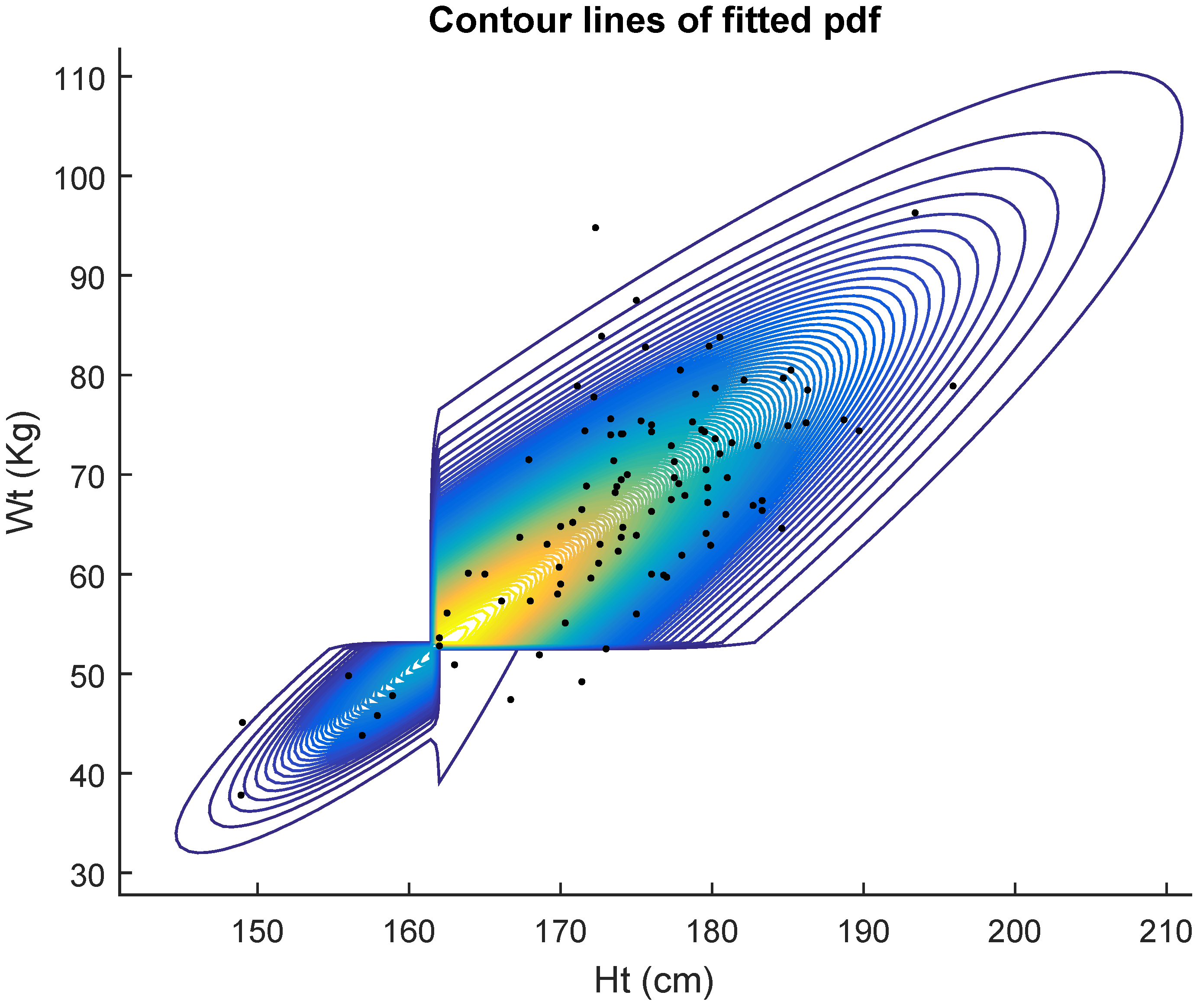
Bivariate Cauchy	$1665.5$	$\left({\mu }_1,{\mu }_2\right)=\left(177.21,69.08\right)$ $\left({\Sigma }_{11},{\Sigma }_{22},{\Sigma }_{12}\right)=\left(77.84,124.86,41.53\right)$	$\left(1.64,2.01\right)$ $\left(2.23,1.39,8.32\right)$

displays the results of the fits for 100 women. In Table 1, we see the results of fitting the five competing models. They are the general bivariate skew$-t$ MH model with pdf given in Equation (9), General bivariate MH with pdf given in Equation (4), Bivariate MH (1.) with pdf given in Equation (5), Bivariate MH (2.) with pdf given in Equation (6) and Bivariate Cauchy. It shows the maximum likelihood estimates (mle’s) of the five models. The last column shows the estimated standard errors (se) of the estimates. Non identifiability of the bivariate skew$-t$ MH model is evidenced by the huge value of the estimated standard error of the estimate of $\nu$. However, the AIC criterion indicates that data are better fitted by the general bivariate skew$-t$ MH (9) model. Figure 2 shows the contour lines of the fitted pdf.

Table 2. Bivariate Mudholkar-Hutson fits for men.

Model	AIC	$\left({\mathit{\alpha }}_{\mathit{i}},{\mathit{\beta }}_{\mathit{i}},{\mathit{\gamma }}_{\mathit{i}},\mathit{\mu },\mathit{\Sigma }\right)$ Estimates	Bootstrap Standard Errors of the Estimates
Bivariate skew t MH	$1396.9$	$\begin{array}{c}\left({\alpha }_1,{\alpha }_2,{\alpha }_3\right)=\left(13.43,20.16,2.62\right)\hfill \\ \left({\beta }_1,{\beta }_2,{\beta }_3\right)=\left(35.02,11.84,6.01\right)\hfill \\ \left({\gamma }_1,{\gamma }_2,{\gamma }_3\right)=\left(0.94,0.96,0.88\right)\hfill \\ \nu =9.99\hfill \\ \left({\mu }_1,{\mu }_2\right)=\left(177.92,70.30\right)\hfill \\ \left({\Sigma }_{11},{\Sigma }_{22},{\Sigma }_{12}\right)=\left(4.77,4.71,4.04\right)\hfill \end{array}$	$\begin{array}{c}\left(14.66,5.34,4.12\right)\hfill \\ \left(8.42,1.82,7.83\right)\hfill \\ \left(0.02,0.02,0.04\right)\hfill \\ 64.18\hfill \\ \left(0.65,1.22\right)\hfill \\ \left(1.89,6.12,1.83\right)\hfill \end{array}$
General bivariate MH	$1441.8$	$\begin{array}{c}\left({\alpha }_1,{\alpha }_2,{\alpha }_3\right)=\left(52.54,52.17,14.58\right)\hfill \\ \left({\beta }_1,{\beta }_2,{\beta }_3\right)=\left(29.83,62.76,31.76\right)\hfill \\ \left({\gamma }_1,{\gamma }_2,{\gamma }_3\right)=\left(0.96,0.98,0.96\right)\hfill \\ \left({\mu }_1,{\mu }_2\right)=\left(174.60,66.6\right)\hfill \\ \left({\Sigma }_{11},{\Sigma }_{22},{\Sigma }_{12}\right)=\left(9.32,17.40,11.78\right)\hfill \end{array}$	$\begin{array}{c}\left(0.89,1.28,0.43\right)\hfill \\ \left(1.52,1.39,0.59\right)\hfill \\ \left(0.01,0.01,0.02\right)\hfill \\ \left(1.13,1.16\right)\hfill \\ \left(0.76,0.50,0.55\right)\hfill \end{array}$
Bivariate MH (1.)	$1456.2$	$\begin{array}{c}\left({\epsilon }_1,{\epsilon }_2,{\epsilon }_3\right)=\left(-0.87,-0.91,-1.0\right)\hfill \\ \left({\mu }_1,{\mu }_2\right)=\left(172.70,61.00\right)\hfill \\ \left({\Sigma }_{11},{\Sigma }_{22},{\Sigma }_{12}\right)=\left(195.26,445.26,279.93\right)\hfill \end{array}$	$\begin{array}{c}\left(0.06,0.05,0.00\right)\hfill \\ \left(1.39,1.94\right)\hfill \\ \left(32.88,62.62,38.52\right)\hfill \end{array}$
Bivariate MH (2.)	$1512.6$	$\begin{array}{c}\epsilon =0.17\hfill \\ \left({\mu }_1,{\mu }_2\right)=\left(185.10,80.54\right)\hfill \\ \left({\Sigma }_{11},{\Sigma }_{22},{\Sigma }_{12}\right)=\left(36.15,70.27,38.53\right)\hfill \end{array}$	$\begin{array}{c}0.21\hfill \\ \left(2.73,3.54\right)\hfill \\ \left(14.66,26.93,19.09\right)\hfill \end{array}$
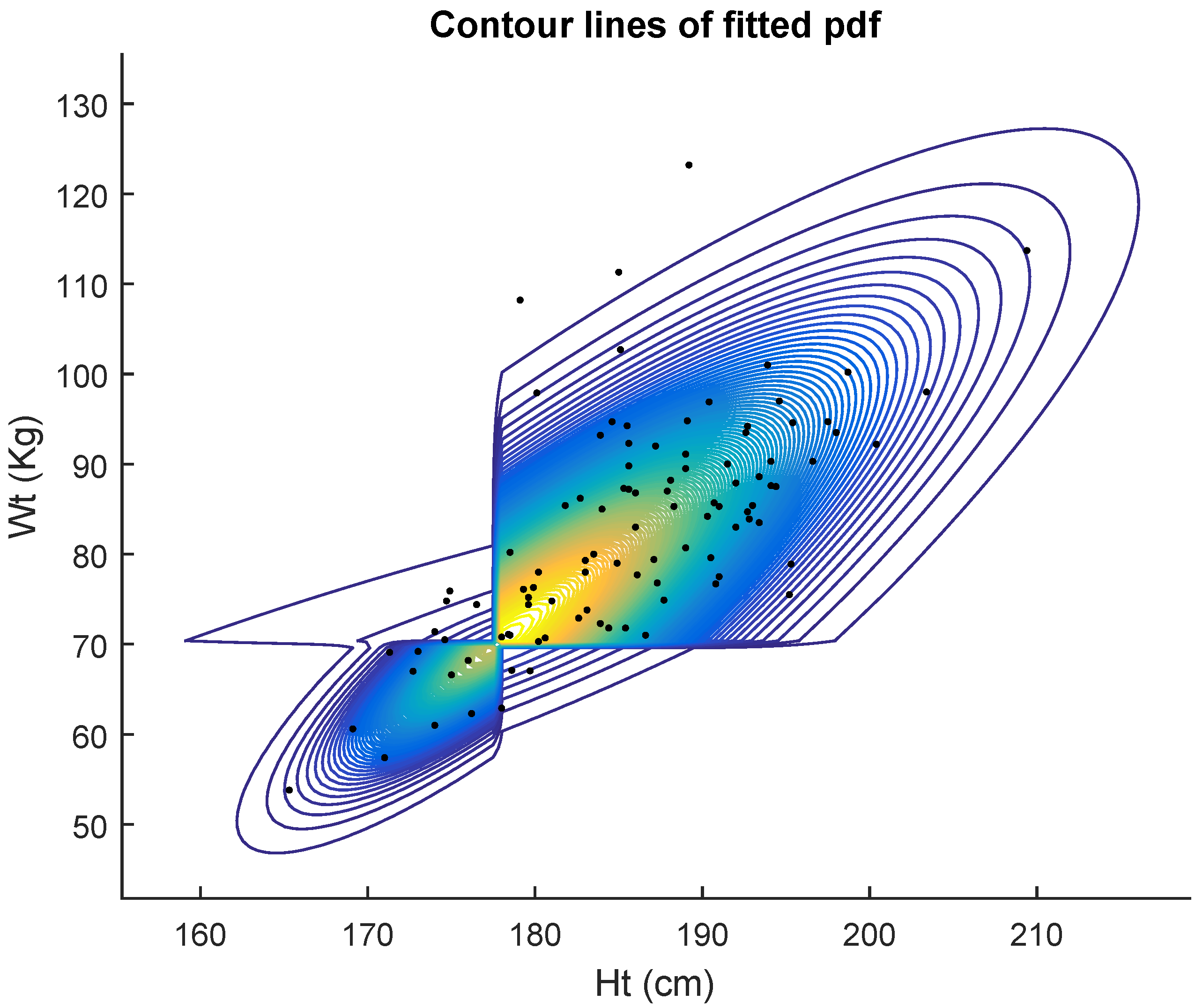
Bivariate Cauchy	$1775.2$	$\left({\mu }_1,{\mu }_2\right)=\left(184.45,79.36\right)$ $\left({\Sigma }_{11},{\Sigma }_{22},{\Sigma }_{12}\right)=\left(65.57,155.19,59.31\right)$	$\left(3.01,3.43\right)$ $\left(3.62,1.54,8.29\right)$

displays the results of the fits for 102 men. In Table 2 we again compare five competing models. The maximum likelihood estimates (mle’s) of the five models, the corresponding Akaike criterion values and estimated standard errors of the estimates are displayed in the table. Again, the AIC indicates that the data are better fitted by the general bivariate skew$-t$ MH (9) model. Figure 3 shows the contour lines of the fitted pdf. Non identifiability of the general bivariate skew$-t$ MH (9) and General bivariate MH (4) models is shown by the large values of the estimated standard errors for some estimates.

Table 3. Bivariate Mudholkar-Hutson fits.

Model	AIC	$\left({\mathit{\alpha }}_{\mathit{i}},{\mathit{\beta }}_{\mathit{i}},{\mathit{\gamma }}_{\mathit{i}},\mathit{\mu },\mathit{\Sigma }\right)$ Estimates	Bootstrap Standard Errors of the Estimates
Bivariate skew t MH	$2803.3$	$\begin{array}{c}\left({\alpha }_1,{\alpha }_2,{\alpha }_3\right)=\left(14.15,17.35,1.09\right)\hfill \\ \left({\beta }_1,{\beta }_2,{\beta }_3\right)=\left(49.35,67.05,1.62\right)\hfill \\ \left({\gamma }_1,{\gamma }_2,{\gamma }_3\right)=\left(0.98,0.96,0.91\right)\hfill \\ \nu =10.93\hfill \\ \left({\mu }_1,{\mu }_2\right)=\left(171.09,61.00\right)\hfill \\ \left({\Sigma }_{11},{\Sigma }_{22},{\Sigma }_{12}\right)=\left(1.01,1.32,1.04\right)\hfill \end{array}$	$\begin{array}{c}\left(8.18,10.35,3.57\right)\hfill \\ \left(5.22,5.57,6.86\right)\hfill \\ \left(0.01,0.01,0.02\right)\hfill \\ 9.42\hfill \\ \left(0.24,0.76\right)\hfill \\ \left(5.74,7.75,6.07\right)\hfill \end{array}$
General bivariate MH	$2901.4$	$\begin{array}{c}\left({\alpha }_1,{\alpha }_2,{\alpha }_3\right)=\left(15.42,17.67,2.25\right)\hfill \\ \left({\beta }_1,{\beta }_2,{\beta }_3\right)=\left(49.28,66.53,3.36\right)\hfill \\ \left({\gamma }_1,{\gamma }_2,{\gamma }_3\right)=\left(0.98,0.96,0.88\right)\hfill \\ \left({\mu }_1,{\mu }_2\right)=\left(170.54,60.95\right)\hfill \\ \left({\Sigma }_{11},{\Sigma }_{22},{\Sigma }_{12}\right)=\left(2.16,3.02,2.35\right)\hfill \end{array}$	$\begin{array}{c}\left(10.74,12.92,2.61\right)\hfill \\ \left(5.00,5.97,5.10\right)\hfill \\ \left(0.01,0.02,0.02\right)\hfill \\ \left(0.54,1.02\right)\hfill \\ \left(1.55,1.84,1.32\right)\hfill \end{array}$
Bivariate MH (1.)	$2984.0$	$\begin{array}{c}\left({\epsilon }_1,{\epsilon }_2,{\epsilon }_3\right)=\left(1.00,0.39,-0.13\right)\hfill \\ \left({\mu }_1,{\mu }_2\right)=\left(181.06,74.48\right)\hfill \\ \left({\Sigma }_{11},{\Sigma }_{22},{\Sigma }_{12}\right)=\left(11.41,50.90,18.73\right)\hfill \end{array}$	$\begin{array}{c}\left(0.01,0.07,0.06\right)\hfill \\ \left(0.76,0.84\right)\hfill \\ \left(1.59,5.00,2.17\right)\hfill \end{array}$
Bivariate MH (2.)	$3022.2$	$\begin{array}{c}\epsilon =0.70\hfill \\ \left({\mu }_1,{\mu }_2\right)=\left(171.37,61.32\right)\hfill \\ \left({\Sigma }_{11},{\Sigma }_{22},{\Sigma }_{12}\right)=\left(48.62,103.69,64.24\right)\hfill \end{array}$	$\begin{array}{c}0.10\hfill \\ \left(2.42,3.07\right)\hfill \\ \left(53.89,89.24,68.07\right)\hfill \end{array}$
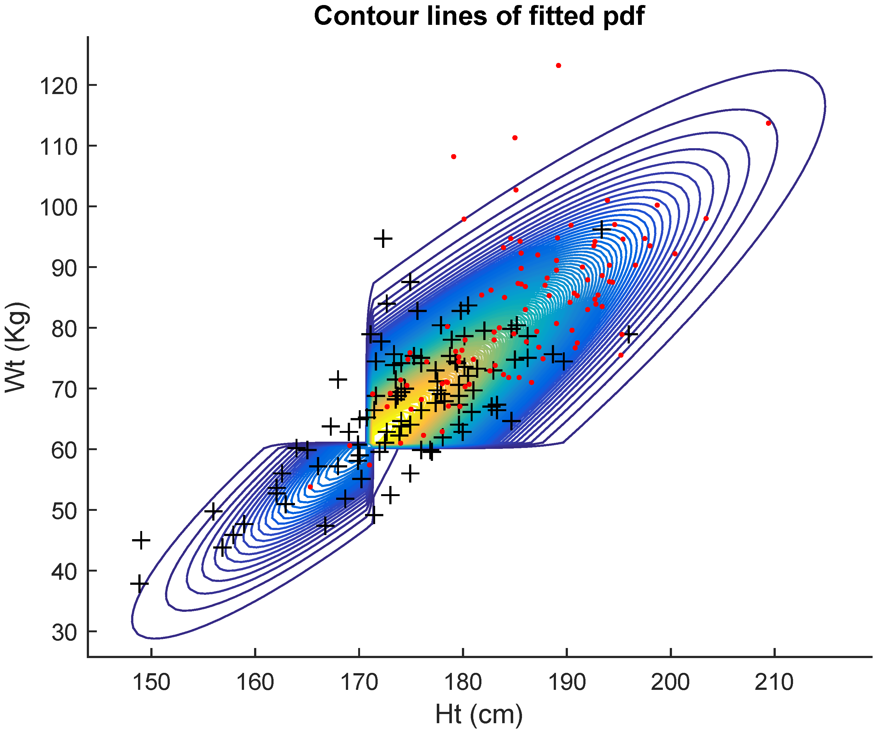
Bivariate Cauchy	$3536.9$	$\left({\mu }_1,{\mu }_2\right)=\left(178.84,71.81\right)$ $\left({\Sigma }_{11},{\Sigma }_{22},{\Sigma }_{12}\right)=\left(106.75,199.84,83.64\right)$	$\left(0.83,1.55\right)$ $\left(2.16,1.16,5.53\right)$

displays the results of the fits for the full set of $n=202$ Australian athletes, regardless of gender. Table 3 shows the maximum likelihood estimates (mle’s) of the five models together with the corresponding Akaike criterion values and estimated standard errors of the estimates. The AIC here also indicates that the data are better fitted by the general bivariate skew$-t$ MH model (9). Figure 4 shows the contour lines of the fitted pdf. Thus, in all three cases, males, females and combined, the best fitting model was the general bivariate skew$-t$ MH.

For the three real cases analyzed the general bivariate skew-t MH model (9) was indicated as the best fitted. That means that it seems worth considering the more general model to explain the variability of these data sets.

6. Concluding Remarks

The Mudholkar–Hutson skewing mechanism admits flexible extensions in both the univariate and multivariate cases. Stochastic representations of such extended models typically have corresponding likelihood functions that are somewhat complicated (for example Equations (4) and (9)). This is partly compensated for by the ease of simulation for such models using the representation in terms of latent variables ( the $U_i$’s and $Z_i$’s in (2) or (8)). The data set analyzed in Section 5 illustrates the potential advantage of considering the extended bivariate Mudholkar-Hutson model, since the basic bivariate M-H model does not provide an acceptable fit to the “athletes” data. Needless to say, applying Occam’s razor, it would always be desirable to consider the hierarchy of the five nested bivariate models that were considered in Section 5, in order to determine whether one of the simpler models might be adequate to describe a particular data set. Indeed there may be other special cases of the model (4), intermediate between (4) and (5) say, that might profitably be considered for some data sets. However, it should be remarked that selection of such sub-models for consideration should be done prior to inspecting the data. The addition of the GBMH model to the data analysts tool-kit should provide desirable flexibility for modeling data sets which exhibit behavior somewhat akin to, but not perfectly adapted to, more standard bivariate Cauchy models.