Time-Fractional Heat Conduction in Two Joint Half-Planes


1
Institute of Mathematics and Computer Science, Faculty of Mathematical and Natural Sciences, Jan Dlugosz University in Czestochowa, Armii Krajowej 13/15, 42-200 Czestochowa, Poland
2
Institute of Mathematics, Faculty of Mechanical Engineering and Computer Science, Czestochowa University of Technology, Armii Krajowej 21, 42-200 Czestochowa, Poland
*
Author to whom correspondence should be addressed.
Symmetry 2019, 11(6), 800; https://doi.org/10.3390/sym11060800
Submission received: 4 June 2019
/
Revised: 13 June 2019
/
Accepted: 14 June 2019
/
Published: 16 June 2019
(This article belongs to the Special Issue Symmetry in Complex Systems)
Abstract
:The heat conduction equations with Caputo fractional derivative are considered in two joint half-planes under the conditions of perfect thermal contact. The fundamental solution to the Cauchy problem as well as the fundamental solution to the source problem are examined. The Fourier and Laplace transforms are employed. The Fourier transforms are inverted analytically, whereas the Laplace transform is inverted numerically using the Gaver–Stehfest method. We give a graphical representation of the numerical results.
1. Introduction
The conventional theory of heat conduction starts from the Fourier law and, coupled with the energy conservation law, implies the conventional parabolic heat conduction equation. In bodies exhibiting complex features, the usual Fourier law and heat conduction equation are not precise enough, and nonstandard theories, in which these equations are substituted by extended (nonlocal) equations, are elaborated.
Time nonlocal equations give an account of memory. Gurtin and Pipkin [1] suggested the general relation between the heat flux vector and the temperature gradient:
In Equation (1), k can be treated as the generalized thermal conductivity, T denotes temperature, t stands for time, and is the weight function.
Nigmatullin [2,3] proposed a similar version of Equation (1):
and obtained for temperature the equation with memory:
In Equation (3), a can be treated as the generalized thermal diffusivity coefficient.
Different choices of the weight function (“full sclerosis”, “short-tail” memory, “middle-tail” memory, “long-tail” memory, and “full memory”) were analized in [4,5,6,7,8].
Though different time nonlocal generalizations of the Fourier law have a long history, they still attract the attention of researchers (see, for example, Reference [9], and the extensive discussion in [10]).
Fractional calculus (the theory of integrals and derivatives of non-integer order) has a large number of uses in engineering, geophysics, physics, geology, chemistry, rheology, biology, finance, and medicine (see [11,12,13,14,15,16,17,18,19,20,21], among many others).
Equation (2), written with the “long-tail” power kernel [4,5,6,7,8], can be represented in terms of fractional calculus:
In Equations (4) and (5), and are the Riemann–Liouville fractional integral and derivative of the order [22,23,24]:
It should be emphasized that in fractional calculus, there is no sharp boundary between integrals and derivatives. This is why some authors [11,22] do not use a separate notation for the fractional integral , which is designated as with . Making use of this notation, Equations (4) and (5) can be depicted as one time-nonlocal relation:
Coupled with the law of conservation of energy, the constitutive relation (8) implies the time fractional heat conduction equation:
with the Caputo fractional derivative:
The interested reader can find the details of obtaining the time fractional heat conduction Equation (9) from the constitutive relation (8) in [25].
Equations (4) and (9) for describe the so-called subdiffusion (slow diffusion), which is characterized by the mean-squared displacement .
In Equations (11)–(13), the asterisk marks the transform, and s stands for the Laplace transform variable.
A variety of boundary conditions for the time fractional heat conduction equation were analyzed in [8,20,26,27]. If the surfaces of two bodies are in perfect thermal contact, the temperatures at their joint boundary S and the heat fluxes through this boundary are the same for both bodies, and we arrive at the following boundary conditions:
where subscripts 1 and 2 mark bodies 1 and 2, respectively, and n is the common normal at the joint surface. In Equation (15), it is assumed that in the general case, the heat conduction in one of the bodies is described by the equation with the Caputo derivative of the order , whereas in the second body, the process is governed by the equation with the Caputo derivative of the order .
In previous publications [27,28,29], the problems of fractional heat conduction in composed bodies were investigated for one spatial coordinate. In the present paper, heat conduction with the Caputo fractional derivative is considered in two joint half-planes under the conditions of perfect thermal contact in the case of two spatial coordinates. The fundamental solutions to the Cauchy and source problems are studied. The Fourier and Laplace transforms are employed. The Fourier transforms are inverted analytically, and the Laplace transform is inverted numerically, employing the Gaver–Stehfest method [30,31,32,33]. The interested reader is also referred to the recent paper [34] on numerical inversion of the Laplace transform for solving fractional deifferenetial equations, where additional references can be found.
2. The Fundamental Solution to the Cauchy Problem
Consider the time fractional heat conduction equations in two half-planes:
We assume the initial conditions:
and the conditions of perfect thermal contact:
The temperatures should also satisfy the zero conditions at infinity:
We introduce the unknown function:
In the subsequent text, we employ the following cos-Fourier transforms with respect to the coordinate x: for :
and for :
Applying to the initial boundary value problem (16)–(27) the Laplace transform with respect to time t, the exponential Fourier transform with respect to the coordinate y, and the foregoing cos-Fourier transforms with respect to the coordinate x, in the transform domain we get is:
All the Fourier transforms are marked by the tilde, denotes the cos-Fourier transform variable, and stands for the exponential Fourier transform variable.
The perfect thermal contact boundary condition (19) written in the transform domain:
makes it possible to determine the function: :
and obtain the expressions for temperatures:
The inverse transforms give:
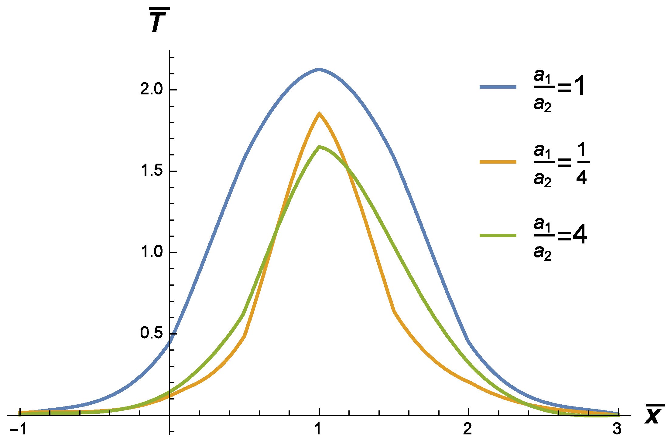
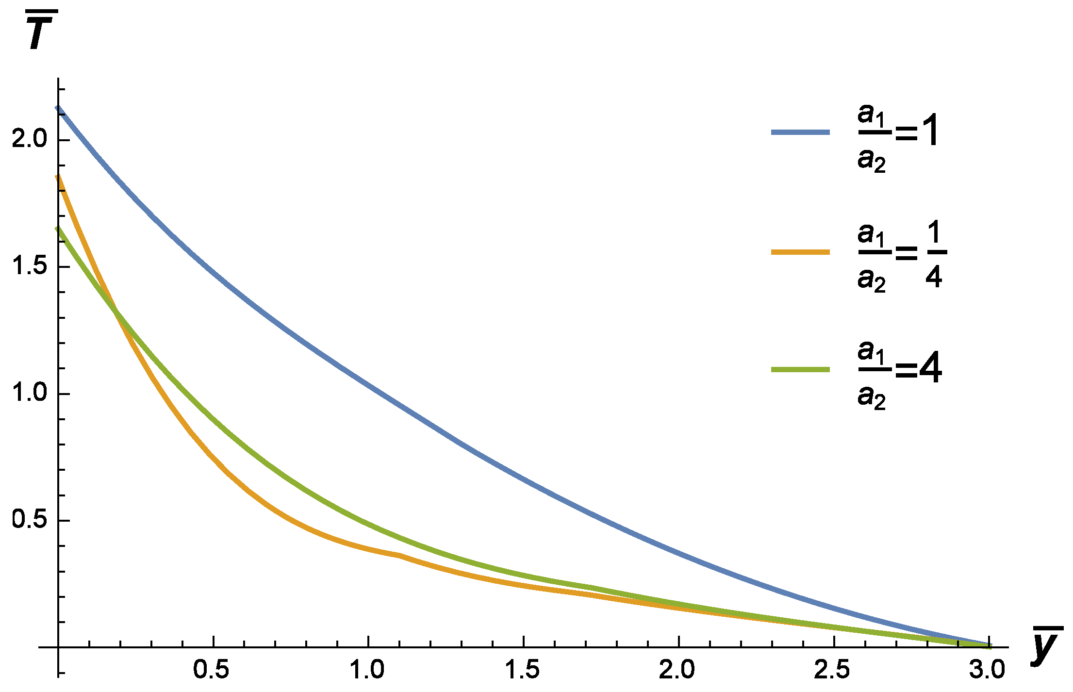
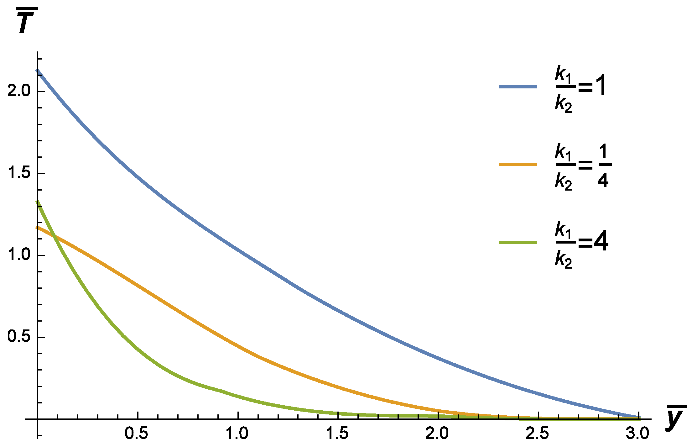
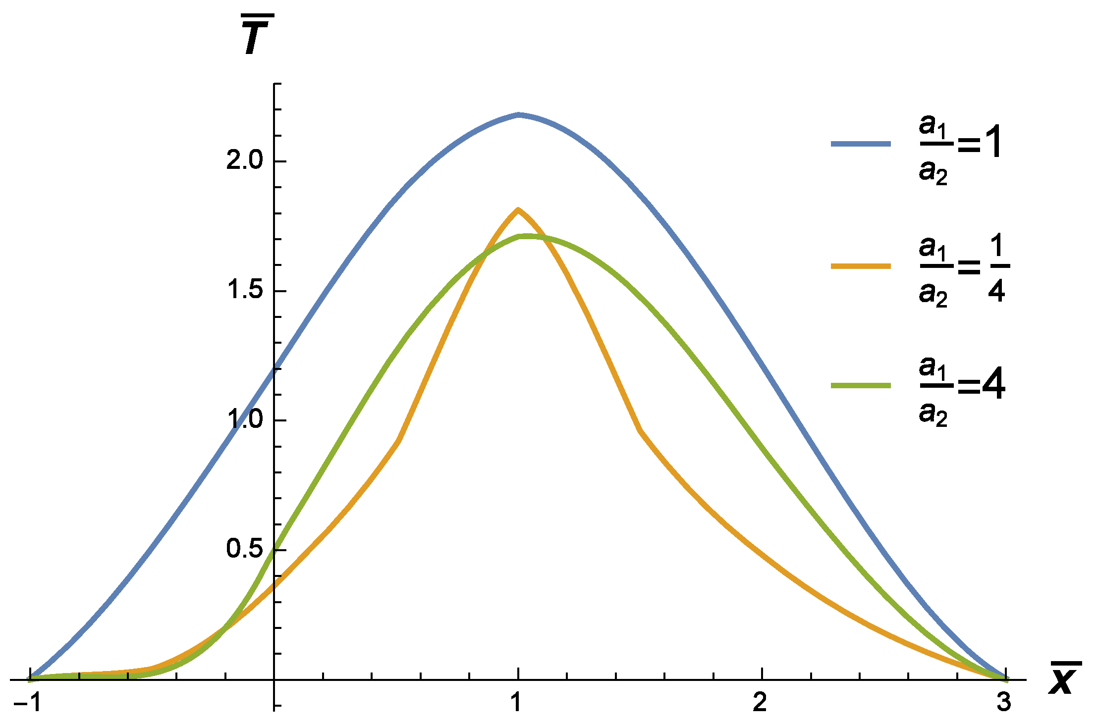
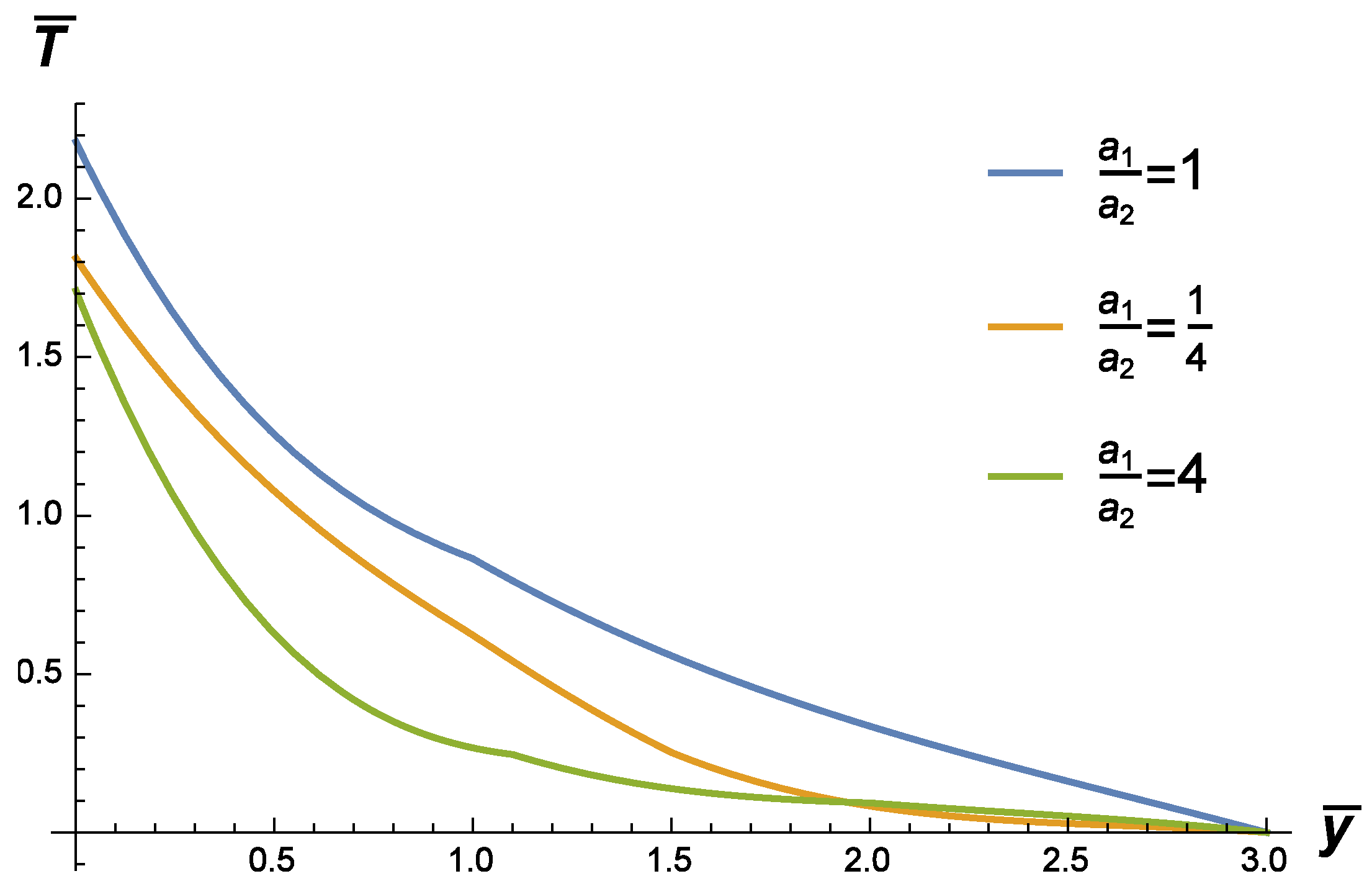
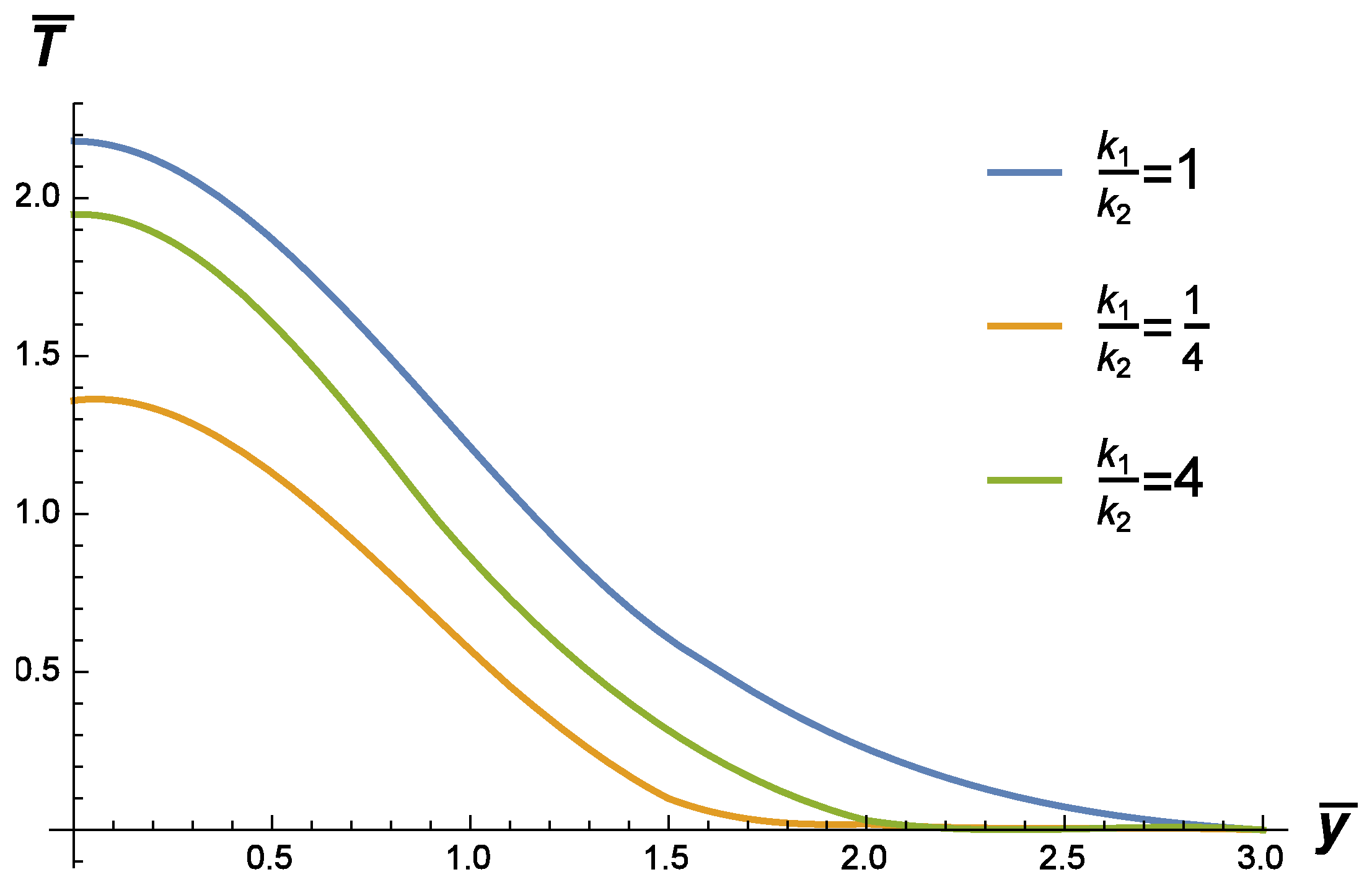
Temperatures in joint half-planes are presented in Figure 1, Figure 2, Figure 3, Figure 4, Figure 5 and Figure 6 for varied combinations of parameters. Calculations have been carried out with the following nondimensional quantities:
where is the characteristic time of the process. In all the figures, the values and have been taken.
3. The Fundamental Solution to the Source Problem
Next, we consider the time fractional heat conduction equation with the source term in the domain :
and the corresponding equation in the region :
We assume the zero initial conditions:
and the conditions of perfect thermal contact at the joint boundary:
Using the integral transform technique, we finally obtain:
4. Conclusions
We studied the heat conduction equations with the Caputo fractional derivatives in two joint half-planes under conditions of perfect thermal contact (the equality of temperatures and heat fluxes at the contact surface). It should be emphasized that due to the constitutive Equation (8), the proper boundary conditions should be stated in terms of the heat fluxes, not in terms of the normal derivatives of temperature alone. Introducing the auxiliary function allows us to use the cos-Fourier transforms in two contact regions. The fundamental solutions permit obtaining various solutions to the Cauchy and source problems in the convolution form.
Author Contributions
Both authors have equally contributed to this work. Both authors read and approved the final manuscript.
Funding
This research received no external funding.
Acknowledgments
The authors would like to thank the reviewers for their helpful comments to improve the quality of the paper.
Conflicts of Interest
The authors declare no conflict of interest.
References
- Gurtin, M.E.; Pipkin, A.C. A general theory of heat conduction with finite wave speeds. Arch. Ration. Mech. Anal. 1968, 31, 113–126. [Google Scholar] [CrossRef]
- Nigmatullin, R.R. To the theoretical explanation of the “universal response”. Phys. Stat. Sol. 1984, 123, 739–745. [Google Scholar] [CrossRef]
- Nigmatullin, R.R. On the theory of relaxation for systems with “remnant” memory. Phys. Stat. Sol. 1984, 124, 389–393. [Google Scholar] [CrossRef]
- Povstenko, Y. Fractional heat conduction equation and associated thermal stresses. J. Therm. Stress. 2005, 28, 83–102. [Google Scholar] [CrossRef]
- Povstenko, Y. Thermoelasticity which uses fractional heat conduction equation. J. Math. Sci. 2009, 162, 296–305. [Google Scholar] [CrossRef]
- Povstenko, Y. Theory of thermoelasticity based on the space-time fractional heat conduction equation. Phys. Scr. 2009, 136, 014017. [Google Scholar] [CrossRef]
- Povstenko, Y. Fractional Cattaneo-type equations and generalized thermoelasticity. J. Therm. Stress. 2011, 34, 97–114. [Google Scholar] [CrossRef]
- Povstenko, Y. Fractional thermoelasticity. In Encyclopedia of Thermal Stresses; Hetnarski, R.B., Ed.; Springer: New York, NY, USA, 2014; Volume 4, pp. 1778–1787. [Google Scholar]
- Rukolaine, S.A. Unphysical effects of the dual-phase-lag model of heat conduction. Int. J. Heat Mass Transf. 2014, 78, 58–63. [Google Scholar] [CrossRef]
- Kovács, R.; Ván, P. Thermodynamical consistency of the dual-phase-lag heat conduction equation. Contin. Mech. Thermodyn. 2018, 30, 1223–1230. [Google Scholar] [CrossRef]
- Magin, R.L. Fractional Calculus in Bioengineering; Begell House Publishers, Inc.: Redding, CA, USA, 2006. [Google Scholar]
- Sabatier, J.; Agrawal, O.P.; Tenreiro Machado, J.A. (Eds.) Advances in Fractional Calculus: Theoretical Developments and Applications in Physics and Engineering; Springer: Dordrecht, The Netherlands, 2007. [Google Scholar]
- Baleanu, D.; Güvenç, Z.B.; Tenreiro Machado, J.A. (Eds.) New Trends in Nanotechnology and Fractional Calculus Applications; Springer: Dordrecht, The Netherlands, 2010. [Google Scholar]
- Mainardi, F. Fractional Calculus and Waves in Linear Viscoelasticity: An Introduction to Mathematical Models; Imperial College Press: London, UK, 2010. [Google Scholar]
- Tarasov, V.E. Fractional Dynamics: Applications of Fractional Calculus to Dynamics of Particles, Fields and Media; Springer: Berlin/Heidelberg, Germany, 2010. [Google Scholar]
- Datsko, B.; Luchko, Y.; Gafiychuk, V. Pattern formation in fractional reaction-diffusion systems with multiple homogeneous states. Int. J. Bifurcat. Chaos 2012, 22, 1250087. [Google Scholar] [CrossRef]
- Uchaikin, V.V. Fractional Derivatives for Physicists and Engineers; Springer: Berlin, Germany, 2013. [Google Scholar]
- Atanacković, T.M.; Pilipović, S.; Stanković, B.; Zorica, D. Fractional Calculus with Applications in Mechanics: Vibrations and Diffusion Processes; John Wiley & Sons: Hoboken, NJ, USA, 2014. [Google Scholar]
- Herrmann, R. Fractional Calculus: An Introduction for Physicists, 2nd ed.; World Scientific: Singapore, 2014. [Google Scholar]
- Povstenko, Y. Fractional Thermoelasticity; Springer: New York, NY, USA, 2015. [Google Scholar]
- Datsko, B.; Gafiychuk, V.; Podlubny, I. Solitary travelling auto-waves in fractional reaction–diffusion systems. Commun. Nonlinear Sci. Numer. Simul. 2015, 23, 378–387. [Google Scholar] [CrossRef]
- Podlubny, I. Fractional Differential Equations; Academic Press: San Diego, CA, USA, 1999. [Google Scholar]
- Kilbas, A.A.; Srivastava, H.M.; Trujillo, J.J. Theory and Applications of Fractional Differential Equations; Elsevier: Amsterdam, The Netherlands, 2006. [Google Scholar]
- Povstenko, Y. Linear Fractional Diffusion-Wave Equation for Scientists and Engineers; Birkhäuser: New York, NY, USA, 2015. [Google Scholar]
- Povstenko, Y. Non-axisymmetric solutions to time-fractional diffusion-wave equation in an infinite cylinder. Fract. Calc. Appl. Anal. 2011, 14, 418–435. [Google Scholar] [CrossRef]
- Povstenko, Y. Neumann boundary-value problems for a time-fractional diffusion-wave equation in a half-plane. Comput. Math. Appl. 2012, 64, 3183–3192. [Google Scholar] [CrossRef] [Green Version]
- Povstenko, Y. Fractional heat conduction in infinite one-dimensional composite medium. J. Therm. Stress. 2013, 36, 351–363. [Google Scholar] [CrossRef]
- Povstenko, Y. Fractional heat conduction in an infinite medium with a spherical inclusion. Entropy 2013, 15, 4122–4133. [Google Scholar] [CrossRef]
- Povstenko, Y. Fundamental solutions to time-fractional heat conduction equations in two joint half-lines. Cent. Eur. J. Phys. 2013, 11, 1284–1294. [Google Scholar] [CrossRef] [Green Version]
- Gaver, D.P. Observing stochastic processes, and approximate transform inversion. Oper. Res. 1966, 14, 444–459. [Google Scholar] [CrossRef]
- Stehfest, H. Algorithm 368 Numerical inversion of Laplace transform. Commun. ACM 1970, 13, 47–49. [Google Scholar] [CrossRef]
- Stehfest, H. Remark on algorithm 368 Numerical inversion of Laplace transform. Commun. ACM 1970, 13, 624. [Google Scholar] [CrossRef]
- Kuznetsov, A. On the convergence of Gaver–Stehfest algorithm. SIAM J. Numer. Anal. 2013, 51, 2984–2998. [Google Scholar] [CrossRef]
- Rani, D.; Mishra, V.; Cattani, C. Numerical inverse Laplace transform for solving a class of fractional differential equations. Symmetry 2019, 11, 530. [Google Scholar] [CrossRef]
- Prudnikov, A.P.; Bryčkov, Y.A.; Maričev, O.I. Integrals and Series, Vol 1: Elementary Functions; Gordon and Breach Science Publishers: Amsterdam, The Netherlands, 1986. [Google Scholar]


© 2019 by the authors. Licensee MDPI, Basel, Switzerland. This article is an open access article distributed under the terms and conditions of the Creative Commons Attribution (CC BY) license (http://creativecommons.org/licenses/by/4.0/).
Share and Cite
MDPI and ACS Style
Povstenko, Y.; Klekot, J. Time-Fractional Heat Conduction in Two Joint Half-Planes. Symmetry 2019, 11, 800. https://doi.org/10.3390/sym11060800
AMA Style
Povstenko Y, Klekot J. Time-Fractional Heat Conduction in Two Joint Half-Planes. Symmetry. 2019; 11(6):800. https://doi.org/10.3390/sym11060800
Chicago/Turabian StylePovstenko, Yuriy, and Joanna Klekot. 2019. "Time-Fractional Heat Conduction in Two Joint Half-Planes" Symmetry 11, no. 6: 800. https://doi.org/10.3390/sym11060800
Note that from the first issue of 2016, this journal uses article numbers instead of page numbers. See further details here.