1. Introduction
In mathematical sciences, graph coloring problems are very easy to state and visualize, but they have many aspects that are exceptionally difficult to solve [
1]. This study traces back to the origin of the four-color problem of whether it is possible to color the regions of every map with four colors such that every two regions having a common boundary are assigned different colors. Later, it was seen that this is a problem in graph theory, whether it is always possible to color the regions of every planar graph (embedded in the plane) so that every two adjacent regions are colored differently [
2]. It took more than 160 years and collective efforts to prove the simple-sounding proposition that four colors are sufficient to color the vertices of a planar graph properly [
3]. Early research in this area was focused mostly on many theoretical aspects, particularly the statements concerning the chromatic number for specific topologies such as planar graphs, line graphs, random graphs, critical graphs, triangle-free graphs, and perfect graphs. Many of the real-world operational research problems can be tackled using graph coloring techniques, and these include disparate problem areas of producing sports schedules, solving Sudoku puzzles, checking for short circuits on printed circuit boards, assigning taxis to customer requests, timetabling lectures at a university, finding good seating plans for guests at a wedding, and assigning computer-programming variables to computer registers [
1].
The harmonious coloring problem of a graph is to find the minimum number of colors needed to color the vertices of a graph such that the color pairs of end vertices of every edge are distinct. Hopcroft and Krishnamoorthy first established the abstraction of the harmonious coloring problem and proved the NP-completeness for general graphs [
4]. Later [
5], one more condition was added that adjacent vertices should receive distinct colors, and the minimum number is called the harmonious chromatic number. This number has been computed for graphs such as paths, two- and three-dimensional grids, complete binary trees, and graphs with a diameter at most two [
5]. Therefore, there were contributions to finding the sharp bound for the graphs such as the collection of non-trivial disjoint paths, disjoint cycles, disjoint complete graphs, the disjoint union of two arbitrary complete binary graphs, trees, triangular snake graphs, double triangular snake graphs, and diamond snake graphs [
6,
7,
8]. Apart from that, Lee and Mitchem [
9] gave an upper bound for the harmonious chromatic number of a graph. As a consequence of this work, there were many improved results on the upper bound in several periods of time [
10,
11,
12,
13]. In [
14], Wang et al. generalized the harmonious coloring problem and called it the local harmonious coloring problem, which is defined as follows.
The local harmonious coloring [
14] is a
d-harmonious coloring if every color-pair is present at most once for every edge within distance
d of any vertex in that graph, and the
d-harmonious chromatic number of
G, denoted by
, is the minimum
k such that
G has a
d-harmonious coloring. Clearly, the original harmonious coloring problem is the
-harmonious coloring problem if
x is the diameter of
G. In addition, it was proven that solving the 1-harmonious coloring problem is NP-complete, and tight bounds were obtained for the path and cycle graphs, whereas the tight bounds for other graphs have been stated as open problems. Recently, Gao [
15] presented three algorithms to give the coloring procedure for the 1-harmonious coloring problem, but these algorithms were based on an exhaustive search of vertices and branching rules.
The above study of the literature justifies the need for systematic mathematical expressions for the 1-harmonious coloring problem. In the present study, we obtained certain tight bounds to compute the 1-harmonious chromatic number. The rest of the paper is organized as follows:
Section 2 contains the lower bound of a graph for the 1-harmonious coloring problem as
, where
is the maximum degree of the graph
G. In addition, we show the exact coloring for a number of graphs, which include grid and honeycomb networks. In
Section 3, we obtain the lower bound for some special classes of graphs for which two or more vertices have
number of common neighbors and show the exact coloring for the complete multipartite, fan, and Benes network. In
Section 4, we connect the coloring numbers of a graph and its subgraph, followed by giving exact coloring for the butterfly network. Finally, we conclude the paper in
Section 5.
2. Lower Bound
We begin this section with an observation that any vertex and all of its neighbors should be colored differently in order to produce the 1-harmonious coloring, and hence, we have the following result.
Theorem 1. Let G be a simple connected graph. Then, .
It would be nice to see the implication of the above bound on basic graph structures such as path
and cycle
on
n vertices each. In fact, the bound is sharp for any path, and interestingly, the bound is not exact for any cycle [
14], as shown in
Figure 1.
We now show the consequences of Theorem 1 for other basic graph structures as given in
Table 1.
Let
be the complete graph on
n vertices. Since each vertex in
is adjacent to all the remaining
vertices, we need
n distinct colors to color
, and it is easy to conclude that
. Similarly, let us consider a star graph
and wheel graph
on
n vertices each. Since the center vertex of star graph (respectively wheel) is adjacent to all the remaining vertices, it is facile to color all the vertices with
n distinct colors. Therefore, we conclude that
, as shown in
Figure 2.
Let T be a tree on n vertices. Without loss of generality, we assume that a vertex v in T has the maximum degree and consider that T is rooted at v. Now, we show that . Color the vertex v with 1 and all the vertices adjacent to v with a color set . Then, color the vertices at the next level, which are adjacent to the already colored vertex with i, using color set . Continue this process till every vertex in the next level of T has been colored using the color set , where j is the color of the vertex at the current level and k is the color of the vertex in the previous level, which is adjacent to j. By Theorem 1, we conclude that .
2.1. Mesh Network
The topological structure of a mesh network is defined as the Cartesian product , , with m rows and n columns.
Theorem 2. For , let G be an mesh. Then, G admits a 1-harmonious coloring with chromatic number + 1.
Proof. We show that + 1 by splitting the proof into two cases. Without loss of generality, we assume that .
Case 1: ( = 2, 2).
In this case, we color the first row vertices from left to right using color order
and the second row vertices by
repeatedly, as shown in
Figure 3. It is clear that for each vertex, its adjacent vertices are colored differently, and by Theorem 1,
.
Case 2: (≥ 3).
We color the row
i,
, by five-color set
from left to right repeatedly as the order described in
Table 2. In what follows,
i (
5) is the remainder of
.
Table 2 shows that any vertex and its adjacent vertices are colored differently, resulting in
. □
2.2. Extended Mesh Network
By replacing each 4-cycle in an mesh into a complete graph on four vertices, we obtain an architecture called the extended mesh and denoted by .
Theorem 3. Let G be an extended mesh (m, n). Then, G admits 1-harmonious coloring with chromatic number + 1.
Proof. It is easy to observe that (2, 2) is a complete graph , and we conclude that . We now show that + 1 by splitting the proof as in Theorem 2. Without loss of generality, we assume that .
Case 1: ( = 2, 2).
We color the first row vertices from left to right using color order
and the second row vertices by
repeatedly, as shown in
Figure 4. It is to be noted that every color pair is present at most once for every edge within distance one, and by Theorem 1,
.
Case 2: (≥ 3).
In this case, we color any row
i,
, by nine-color set
from left to right repeatedly as the order described in
Table 3, and our coloring method results in
. □
2.3. Generalized Honeycomb Network
The generalized honeycomb network [
16] can be built from an infinite hexagonal system with no cut vertices or non-hexagonal interior faces. It is denoted by
, and the structure can be developed using hexagons in various ways by fixing the parameters as
,
,
, and
, as shown in
Figure 5. In particular, it generates the honeycomb network when
.
Theorem 4. Let G be the generalized honeycomb network . Then, G admits 1-harmonious coloring with chromatic number .
Proof. We show that
by considering the elementary horizontal edge cuts
,
, as shown in
Figure 6. The removal of all
’s in G results in
number of paths and represented by
,
. Let
be the first vertex of
. We now define a labeling function
l from
into
as follows:
We now color the vertices of the paths
by
from left to right repeatedly as the order described in
Table 4. By this coloring method and Theorem 1, we arrive at
. □
3. Tight Bounds on Some Special Classes of Graphs
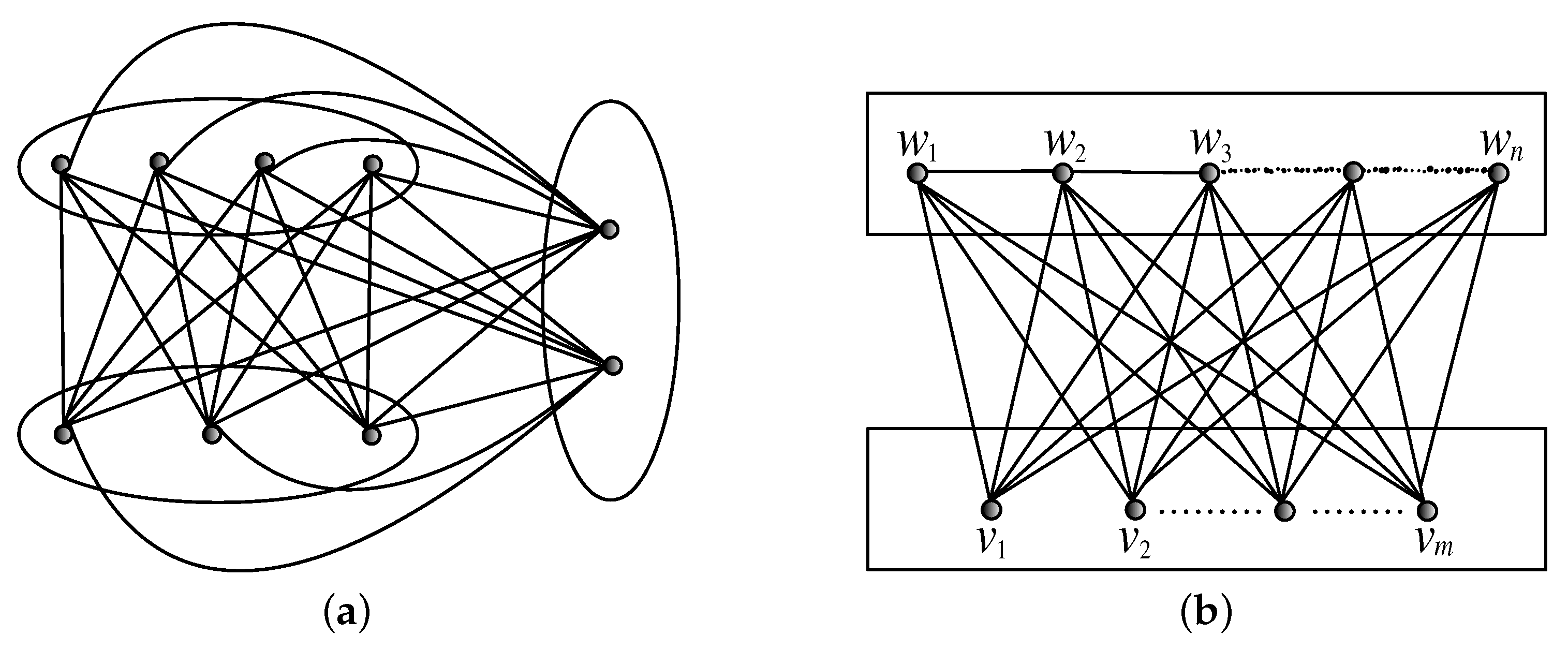
We begin this section by giving the definitions of the complete multipartite graph and fan graph. A graph
is a
t-partite,
, if it is possible to partition
into
t disjoint subsets
such that every edge in
joins a pair of vertices that come from two different partite sets. A complete multipartite graph
G is a
t-partite graph such that there is an edge between every pair of vertices from different partites and denoted by
, where
is the cardinality of
,
, See
Figure 7a. A fan graph
is obtained from
by joining all the vertices in the second partite by a unique path, See
Figure 7b.
Theorem 5. For , let G be a connected graph such that k number of vertices have number of common neighbors. Then, .
Proof. Let be the vertices of G such that each has number of common neighbors , . Without loss of generality, we color the vertex as 1. Then, it is obvious that the neighbors of should be colored with colors different from the color 1. Since each is adjacent to all the vertices , we are forced to give the new colors to the vertices . Hence, . □
We now show the implication of the above theorem on some special classes of graphs such as a complete multipartite, fan graph, and Benes network.
Theorem 6. The 1-harmonious coloring number of complete multipartite and fan graphs is given by and .
Proof. As , it is enough to prove that . Since and from the construction of the complete multipartite graph, we observe that number of vertices have common neighbors, and by Theorem 5, we arrive at . Similarly, we can prove the fan graph. □
In what follows, is the binary hypercube of dimension n and . For any positive integer and r, we denote and .
The
n-dimensional butterfly network, denoted by
, has a vertex set
, and two vertices
and
are connected by an edge if and only if
and either
or
x and
y differ precisely in the
bit. Clearly,
x and
i represent the row and the level (column) of the vertex
respectively, and the two-dimensional butterfly is depicted in
Figure 8a. Further, the butterfly network was extended by adding
n more levels, and resulting network is called the Benes network. Clearly, the
n-dimensional Benes
has
levels with
vertices in each level. The vertices from Level 0 to level
n (respectively,
n to
) in
induce a
, and hence, the middle level of the Benes network is shared by two copies of butterfly networks [
17], as shown in
Figure 8b.
We now notice that Theorem 5 is extremely useful in proving a sharp bound for the Benes network and not in the case of the butterfly network, which is dealt with separately in the next section.
Theorem 7. The Benes network admits 1-harmonious coloring with chromatic number .
Proof. From the definition of the Benes network, we have
, and we further identify that the vertices
and
of
have four common neighbors. Theorem 5 implies that
. We now show that
by defining a labeling function
l from
into
as follows:
Since
, we color the vertices at the
level as
from top to bottom. Now, we color the vertices at the remaining levels using six-color set
as the order described in
Table 5.
Since all the vertices in each level are independent and each vertex
has its neighborhoods only at the levels
and
, the vertices of any three consecutive levels are colored with three distinct pairs of colors
,
and
, respectively shown in
Figure 9, and we have
. □
4. The 1-harmonious Coloring of the Butterfly Network
In this section, we first state the natural property of 1-harmonious coloring and then give the exact coloring for butterfly networks.
Theorem 8. Let H be a subgraph of the graph G. Then, .
Theorem 9. The butterfly network admits 1-harmonious coloring with chromatic number: Proof. Since is , we have . We now show that cannot be colored with five colors. Without loss of generality, let the color of vertex be . Then, its neighboring vertices and should be colored from the color set in some order. Again, without loss of generality, we assume that , , and . In this case, the vertices and can be colored in the following ways:
- (i)
or 5,
- (ii)
or 3.
We start with the first case
and
. Since
, we can color the vertices
and
using the color set
in some order. Let us assume that
and
. Similarly, since
, we can color the vertices
and
using the color set
in some order. However, whatever may be the order, the vertex
is now adjacent to two vertices colored with 1. Therefore,
. In the same manner, we can prove the other three cases that
, as shown in
Figure 10.
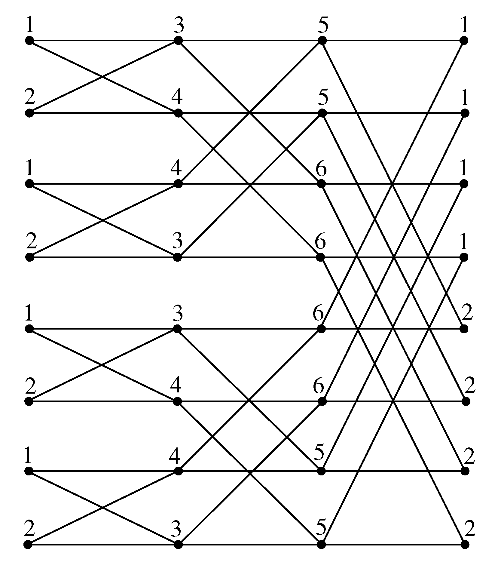
By Theorem 8, we have
, and we now color the vertices of
with six colors. First, we color the vertices at Level 0 as
from top to bottom. Now, we color the vertices at the remaining levels using six-color set
as the order described in
Table 6.
The way in which we colored the butterfly network is similar to the Benes network, and following the proof technique of Theorem 7 as illustrated in
Figure 11, we arrive at
. □


