Abstract
Industrial Control Systems (ICSs) are widely used in critical infrastructures to support the essential services of society. Therefore, their protection against terrorist activities, natural disasters, and cyber threats is critical. Diverse cyber attack detection systems have been proposed over the years, in which each proposal has applied different steps and methods. However, there is a significant gap in the literature regarding methodologies to detect cyber attacks in ICS scenarios. The lack of such methodologies prevents researchers from being able to accurately compare proposals and results. In this work, we present a Methodology for Anomaly Detection in Industrial Control Systems (MADICS) to detect cyber attacks in ICS scenarios, which is intended to provide a guideline for future works in the field. MADICS is based on a semi-supervised anomaly detection paradigm and makes use of deep learning algorithms to model ICS behaviors. It consists of five main steps, focused on pre-processing the dataset to be used with the machine learning and deep learning algorithms; performing feature filtering to remove those features that do not meet the requirements; feature extraction processes to obtain higher order features; selecting, fine-tuning, and training the most appropriate model; and validating the model performance. In order to validate MADICS, we used the popular Secure Water Treatment (SWaT) dataset, which was collected from a fully operational water treatment plant. The experiments demonstrate that, using MADICS, we can achieve a state-of-the-art precision of 0.984 (as well as a recall of 0.750 and F1-score of 0.851), which is above the average of other works, proving that the proposed methodology is suitable for use in real ICS scenarios.
1. Introduction
Industrial Control Systems (ICSs) are the core of critical infrastructures that provide essential services such as water, power, or communications, among others. ICSs support basic services for monitoring and controlling industrial processes. On the one hand, the monitoring part supervises the processes and checks their correct operation through the measurement of different signals obtained by sensors. On the other hand, the controlling part manages the processes and makes decisions that trigger actions carried out by actuators. If this workflow is interrupted due to technical problems or cyber attacks, many citizens can be affected; for example, through disruptions of electrical supply or communications.
ICS are complex systems, whose networks transport sensor and actuator information together with multimedia data [1], such as images and videos. Thus, it is crucial to adopt security mechanisms to protect these information assets from malicious activities and cyber threats. These cybersecurity mechanisms are needed not only to maintain service availability, which is critical to sustain the supply chain, but also to ensure the safety of workers and goods and protect the information—either sensor/actuator or multimedia data—which flows in their networks. On the one hand, an ICS affected by a cyber attack can trigger a malfunction, causing some physical part (e.g., a robotic arm or a whole robot) to damage other physical elements or even people. On the other hand, a cyber attack can steal confidential information about the process performed in the industry, which can ultimately reduce industrial competition.
Over the years, multiple cyber attacks and incidents have been reported in the ICS field [2,3]; however, their incidence has been increasing [4]. Among them, we highlight the Stuxnet [5] malware, which infected nuclear plants in Iran, and Irongate [6], a Stuxnet-based malware developed to attack ICSs specifically. This increase can be explained by the following reasons:
- Increased connectivity to the Internet [7] and the integration of commercial-off-shelf technologies (COTS) [8], which expose ICSs to vulnerabilities similar to those typical of IT networked systems.
- The value attached to ICSs by critical infrastructure stakeholders, given the contribution of ICSs to cyber-physical system interactions and interdependencies, and the damage that interferences can cause [9].
Due to the increase of cyber attacks, researchers have proposed many techniques to detect and mitigate cyber attacks affecting ICSs. Intrusion Detection Systems (IDSs) [10], together with Intrusion Prevention Systems (IPSs) [11] are popular systems to detect and mitigate cyber attacks in corporate networks. They monitor network traffic, in order to detect and prevent intrusions, using traditional techniques. However, these traditional systems rely on databases that store the signatures of well-known cyber attacks, in order to compare the monitored traffic with those signatures. In other words, to detect a cyber attack, it must have been seen previously and its signature stored in the database. The main consequence is that these techniques are inefficient in detecting specialized or unseen cyber attacks. In order to address these limitations, the anomaly detection paradigm has moved to Deep Learning (DL) and Machine Learning (ML) methods, which can achieve high performance in terms of evaluation time [12]. The anomaly detection paradigm is usually considered to detect cyber attacks, as a cyber attack is an event that rarely occurs and, so, can be considered as an anomaly. Although many anomaly detection methodologies based on ML/DL have been proposed in different fields, industrial scenarios have several considerations that need to be taken into account in order to detect an anomaly successfully. Therefore, the current major challenge is the lack of a common methodology in the anomaly detection field that establishes guidelines to detect cyber attacks specialized in ICS scenarios. The existing solutions apply different steps without standard criteria, resulting in hardly comparable results. The lack of such a common methodology may even lead to the results obtained by the researchers being invalid, due to the wrong steps being carried out.
To overcome the aforementioned challenge, we propose a Methodology for Anomaly Detection in Industrial Control Systems (MADICS), a complete methodology based on semi-supervised ML and DL anomaly detection techniques for the ICS field. MADICS is intended to be a step-by-step guide that any researcher can apply to detect cyber attacks in ICS scenarios, aiming to provide a common and unified means to compare results in the field of cyber attack detection in ICS scenarios. Although the MADICS steps are based on a typical ML/DL methodology, it is worth mentioning that these steps are adapted to industrial scenarios and can deal with the specific particularities present in these types of scenarios. Among these particularities that other scenarios such as 5G networks [13] or clinical information systems [14] do not have, we highlight the high correlation between the features and the repetitiveness of actions carried out in ICS. To address these issues, MADICS proposes specific actions for an ICS scenario, such as the study of the correlation between features and the label, not to eliminate features, but to determine if a data leakage has occurred, and the application of two different techniques to extract high-order features based on the repetitive nature of the ICS. The proposed methodology is divided into the following steps and assumes that an ICS-oriented dataset is available.
- Cleaning the dataset to be used with ML and DL models. Dataset splitting, categorical feature encoding, corrupt and missing value treatment, and feature scaling are some of the tasks considered in this step.
- Filtering features to select the most discriminant ones. Features with high correlation, with no variance, or anomalous behavior are removed.
- Extracting higher order features from the dataset. This process exploits the repetitive nature of ICSs and uses statistical measures to extract features from autocorrelation and the Discrete Fourier Transform (DFT).
- Building an anomaly detection method. First, a prediction model and hyperparameters are selected, and then, the optimal ones are searched. Second, the prediction model is trained, and finally, a threshold is selected to decide whether a certain sample comes from the normal system behavior or a cyber attack.
- Validating the results obtained using performance metrics such as precision, recall, and F1-score.
In addition, we validated MADICS using the popular SWaT [15] dataset, which was collected from a fully operational water treatment plant. The performed validation tests achieved a precision of 0.984, which is the highest precision compared with related works. Moreover, the recall and F1-score were 0.750 and 0.851, respectively, which are above the average values obtained in other works. In terms of cyber attack detection, MADICS identified 23 of 28 cyber attacks, proving that MADICS is suitable for real ICS scenarios.
The remainder of this paper is organized as follow: Section 2 presents a literature review in relation to ML and DL solutions focused on cyber attack detection in ICSs. In Section 3, we present the proposed methodology for cyber attack detection in ICS scenarios. This section is split into five sub-sections, in which each step of the methodology is explained. In Section 4, we show the implementation of our methodology using the well-known SWaT dataset. In Section 5, we discuss our findings. Finally, the conclusions and future work are presented in Section 6.
2. Related Work
In the past, many solutions have been proposed to detect cyber attacks in ICSs. Some examples are the usage of rule-based IDSs [16,17,18] or Deterministic Finite Automata (DFA) [19]. However, at present, research efforts are typically focusing on developing new techniques using innovative technologies such as Big Data [20] or ML/DL. In particular, the use of ML and DL techniques is increasing, which play a key role in detecting cyber attacks affecting the industrial field [21]. This section performs an exhaustive review of the most relevant works related to ML/DL for anomaly detection in the industrial context. After this revision, we see that the existing solutions follow different methodologies and procedures, without clear guidelines. A summary of the main aspects of these works is listed in Table 1.

Table 1.
Overview of the different works focusing on anomaly detection in Industrial Control System (ICS) scenarios. Each column corresponds to the steps that we considered desirable to detect cyber attacks in ICS scenarios. DIF, Dual Isolation Forest.
Due to its nature, anomaly detection in ICSs is frequently treated as a time-series classification problem. Therefore, many techniques rely on algorithms that can deal with time. Among these DL techniques, we highlight Convolutional Neural Networks (CNN) and Long-Short Term Memory (LSTM) neural networks. Both can be applied to problems that require converting the input data into sequences, and both can deal with the concept of time; for example, in [22], the authors tested different DL models to detect anomalies. Among the tested methods, we outline the LSTM and 1-Dimensional Convolutional Neural Network (1D CNN). Besides, the authors proposed adding new features by computing the difference between the current value and the past values with a given lag. The authors concluded that 1D-CNN obtained a better result than LSTM, while being much faster to train. Another example is [23], where the authors proposed an automatic architecture optimization based on Genetic Algorithms (GAs). The DL models tested by the authors were Dense Neural Network (DNN), 1D-CNN, and LSTM networks. In addition, the authors proposed the usage of the Numenta Anomaly Benchmark (NAB) metric [24], instead of the F1-score, and introduced different threshold methods such as exponentially weighted smoothing, mean p-powered error measure, individual error weights for each variable, and disjoint prediction windows. In [25], an IDS based on the LSTM neural network was presented. The authors proposed a Cumulative Sum (CUSUM) method for anomaly detection. The CUSUM is computed from the residual error calculated from the ground-truth and the data predicted by the model. A novel Generative Adversarial Network-based Anomaly Detection (GAN-AD) method for ICS scenarios was presented in [26]. The authors implemented an LSTM network in the core of the GAN-AD to capture the distribution of the multivariate time-series of sensors and actuators under normal conditions in an ICS. Another example using LSTM networks is [27], where the authors proposed a sequence-to-sequence LSTM neural network for anomaly detection. The LSTM network was trained using data under normal conditions and made use of attention mechanisms.
In addition to CNN and LSTM networks, other DL and ML techniques have been proposed in the literature. For example, in [28], the authors proposed and evaluated the application of unsupervised machine learning to detect anomalies in Cyber–Physical Systems (CPS). They compared two different methods: Deep Neural Network (DNN) and Support Vector Machine (SVM). Both are adapted to work with time-series data. They scaled the test dataset with its own mean and standard deviation. In [29], the authors proposed a DL method based on AutoEconders (AE) and 1D-CNN for anomaly detection in ICSs. In addition to the DL models proposed by the authors, they suggested filtering features to select those more suitable for the anomaly detection task. They also introduced a feature extraction process that computes features in the frequency domain using the Discrete Fourier Transform (DFT). However, feature extraction using the DFT creates features based on the most energy bands, removing important information from the remaining signal. Besides, they used a threshold for anomaly detection defined as a function of the mean and standard deviation of the test dataset. The authors of [30] presented an unsupervised anomaly detection method focused on large-scale and real-time data analysis. The approach is based on three techniques: an update trigger, tree growth, and a mass weighting scheme. This combination allows for online updating and building the random trees. Another unsupervised anomaly detection was presented in [31], where the authors conducted clustering analysis to find the underlying structures present in the dataset. Next, the authors extracted features from the clusters considering cluster intra-distances and inter-distances. Finally, an inference system determined whether an anomaly was triggered. In [32], the authors presented an unsupervised learning approach based on stacked denoising autoencoders. Their approach used the bytes of the original network stream; therefore, it does not require specific knowledge.
The authors of [33] presented a semi-supervised approach based on Dual Isolation Forest (DIF). In this approach, two Isolation Forests (IF) are trained. The first IF is trained with the original data after normalizing, while the second IF is trained with a version of the original data after applying the Principal Component Analysis (PCA) technique. Additionally, they used the normal samples from the training and test datasets to train the model; while, to test the model, they only used cyber attack samples from the test dataset. In [34], the authors developed another anomaly detection IDS using ML algorithms – Naive Bayes, PART, and Random Forest (RF) – and performed a feature extraction process to improve their results. Similarly, the authors of [35] presented an IDS based on three models of machine learning (J48, naive Bayes, and RF) to detect Distributed Denials of Service (DDoS) in SCADA systems. In [36], the authors generated a new dataset collected from an electric traction sub-station and tried semi-supervised and supervised ML and DL models to detect anomalies. Among the models tested, we highlight RF, Support Vector Machine (SVM), One-Class Support Vector Machine (OCSVM), IF and DNN. In their work, the authors encoded categorical features and normalized features.
As can be seen in Table 1, there is no standardized procedure, and the steps of each work have been left to the authors’ discretion. Moreover, if we extend our analysis to anomaly detection methodologies using other types of techniques, there is a reduced number of additional works; for example, ref. [37] proposed an independent methodology to analyze an Internet of Things (IoT) data stream in real time, presenting a proof-of-concept in the form of anomaly detection. In [38], the authors presented an anomaly detection methodology using boosted regression trees. There are only a few methodologies proposed in the literature for ICS cybersecurity. In particular, the authors of [39,40] proposed two methodologies for gas turbines. The former presented the k-σ methodology, whereas the latter presented an optimization over the k-σ methodology. Both of them rely on the mean and standard deviation, however detecting only a limited kind of cyber attacks.
In conclusion, the majority of the related work have proposed new anomaly detection techniques based on a different ML/DL models, but without following a methodology that establishes guidelines to detect cyber attacks. Thus, there is a clear gap in terms of methodologies that allow the development of ML and DL models for the detection of cyber attacks in ICS scenarios. In our work, we propose a complete methodology that allows future works to follow a sequence of common steps.
3. Proposed Methodology
This section describes MADICS, which is divided into the five steps: (1) dataset pre-processing, (2) feature filtering, (3) feature extraction, (4) anomaly detection method selection, and (5) validation. A graphical representation of the methodology is shown in Figure 1.

Figure 1.
Methodology for anomaly detection in ICSs.
Although these five steps are common to every ML/DL project, we recommend taking very specific tasks and optimal actions for our scenario (i.e., industrial control systems). ICSs have specific characteristics that are important to consider when designing an anomaly detector. Among these characteristics, we highlight the repetitive nature of the ICS and the need to preserve the temporal coherence in both dataset splitting and model training. Besides, in other contexts different from ICSs, a high correlation between features would be an indicator of a problem, and it should be necessary to remove those features. However, because of the high dependence between the devices in ICS, high correlation is desirable, and therefore, it does not indicate any issue. In contrast, a high correlation between the vector label and features would indicate a potential issue. Our methodology considers this characteristic of the ICS, and particular actions are recommended when a high correlation is found between the features and the vector label.
3.1. Dataset Pre-Processing
In this section, we start from a dataset obtained directly from the selected ICS scenario. Although the methodology is based on a semi-supervised approach, it requires a labeled dataset to validate the results properly. The main goal of this first step is to prepare the dataset to be used with semi-supervised ML and DL models.
The first task is to perform the dataset division into three new datasets: training, validation, and test. The training dataset is used to train the model, the validation dataset to evaluate the performance of the model during hyperparameter optimization, and the test dataset to validate the methodology with unseen data. If the dataset is not initially partitioned into training, validation, and test sets, we need to follow some criteria to obtain a suitable partition. MADICS imposes two restrictions: (1) the training dataset must contain only normal data, whereas the test dataset must contain normal and anomalous data; and (2) the temporal order in the dataset must be preserved. Therefore, the value of certain features should depend on the evolution over time of other features: for example, at an instant t, the water tank output valve is open because, during the previous instant, , the water tank input valve was open and the water tank was filling. Moreover, we recommend partitioning the dataset by taking the initial samples for the training dataset and the remaining samples for the test dataset. Once the training dataset is obtained, we need to extract a small partition as the validation dataset. An established method is to split the original training dataset into two new datasets following the 80/20 rule [41], while still preserving the temporal order. Conversely, if the dataset is already partitioned, we should use that division to train, validate, and test our models, to be able to compare our results with others using the same dataset.
The second task is to explore the dataset, in order to check whether the data contain spurious or corrupted values. These types of values are frequent during transitory states or warm-up processes; that is, when the ICS is initializing or after a cyber attack is performed. We suggest independently plotting each feature against time and visually identifying corrupted values to remove the corresponding samples. Additionally, we also recommend checking whether the dataset contains missing values and to fix them accordingly. To treat missing values, there are three well-known techniques: (1) set missing values to the mean/median; (2) remove the damaged samples; and (3) mark the missing values as non-valid data. The first two options are not appropriate in an ICS dataset. First, many features in ICS datasets are categorical (i.e., they only contain a few discrete values, such as a valve being either open or closed), and the usage of the mean/median makes no sense for these values. Second, the absence of a value can contribute information about the cyber attack (e.g., a cyber attack that halts a valve controller). Therefore, we recommend marking missing values as not valid, either by setting them to an invalid value or adding a new column to the dataset that indicates the validity of the data.
The third task is dedicated to the preparation of categorical features to be used with the ML and DL models. At this point, our suggestion is to encode categorical features present in the dataset by applying One-Hot Encoding (OHE), yielding a binary feature for each different categorical value. As an example, consider a valve feature with three possible states: open, half-open, and closed. This feature is replaced, after applying OHE, by three binary features representing the open, half-open, and closed valve states, respectively. An optional embedding layer would transform the set of OHE categorical features into a vector of continuous features. This transformation allows for better integration of both types of features into the neural network, which might improve the detection results [42].
The fourth and final task consists of scaling the continuous features. We recommend two different approaches: standardization and min-max scaling. Standardization is the best option when the data follow a normal distribution. For each continuous feature in the training set, the mean is subtracted, and the resulting values are divided by the standard deviation. The same mean and standard deviation computed on the training set is used to standardize the test dataset. After applying standardization, each feature has a zero mean and unit variance. The advantage of min-max scaling is that it does not distort the dataset shape. We first calculate the maximum and minimum values in the training dataset, and then, we scale both the training and test datasets by subtracting the minimum value and dividing by the difference between the maximum and minimum values. After applying this normalization, each feature is within the range of [0, 1].
3.2. Feature Filtering
In this section, we propose several techniques to study the features of the dataset. The goals of these techniques are twofold: To determine if data leakage is present in the dataset and the elimination of features that do not change in the entire dataset, as well as those whose statistical distributions in the training, validation, and test datasets differ significantly.
The first task consists of studying features that have a high correlation with the vector label (indicating the presence or absence of cyber attack). Although features in an industrial dataset are extracted from physical signals and are supposed to be coherent, the dataset creation and pre-processing steps may introduce some data leakage, which must be studied. In ICS datasets, features are frequently correlated. As an illustration, when a sensor reports that a particular water tank is full, usually the pump controlling the water tank input stops or the pump controlling the water tank output opens. This kind of correlation is normal and desirable in the anomaly detection context. In contrast, a high correlation between specific features and the vector label needs further analysis, as it likely signals the presence of some kind of data leakage. If the data leakage possibility is discarded, then the high correlation found means that the problem is simple enough to use rule-based systems. In contrast, if data leakage is suspected, our suggestion is to discard the feature. We recommend using the Pearson correlation coefficient to estimate the correlation between features, considering that a high correlation exists when its absolute value is above 0.9.
The second task consists of figuring out the features that do not change in the dataset and removing them. We recommend testing each feature in the original dataset using a variance threshold and then preserving only those features with sufficient variance.
The third and final task is to check whether the features in the training and test datasets follow the same statistical distributions; otherwise, our model will be unable to predict accurately. In that case, we should extend our (training and test) datasets with more data, in order to unify their distributions. If there is no possibility of obtaining more data, we can attempt to use only those features whose distribution remains sufficiently stable. In order to check for the similarity between continuous empirical distributions, we recommend applying the well-known Kolmogorov–Smirnov (K-S) test. The K-S statistic quantifies the distance between two continuous distribution functions. The smaller the distance, the more similar the distributions. We suggest applying K-S to remove those features whose continuous distribution is not preserved between training and test datasets; that is, those features with a distance greater than a given threshold. Nevertheless, even if we have sufficient data with the same distribution in the training and test sets, we need to keep in mind that an ICS is a dynamic system, and its normal pattern of behavior can evolve over time (and with it, the statistical distribution of the features), requiring periodic re-training to update the model.
3.3. Feature Extraction
Feature extraction is the process of using expert knowledge to extract higher order features from the original features. In this section, we detail the tasks needed to obtain those higher order features, considering that ICSs are intended to control industrial and critical processes, which frequently perform repetitive actions. For example, an ICS that controls and monitors a water tank should consider the lower and upper water tank limits to consequently open and close the input and output water valves. This action is repeated over time, as the water reaches its lower and upper limits. These repetitive actions are reflected in the logs from which the datasets are created. To determine these repetitive actions, in the form of features, we recommend extracting features using autocorrelation and the Fourier Transform (FT).
The first task is to use an autocorrelation function to extract higher order features. Autocorrelation is defined as the correlation of a signal with a delayed copy of itself, as a function of the delay k (lag). In our case, the correlation is applied over a time window of length W. The formal definition of the autocorrelation is shown in Equation (1), where denotes the value of x at an instant w and is the mean of the x values in the window. One of the multiple practical applications of autocorrelation is to find repeating patterns. Hence, we expect to extract features related to signal pattern repetition in sensors and actuators:
The second task is to use FT to extract higher order features. FT is a mathematical tool that decomposes a signal into the frequencies from which it is formed. In other words, the FT allows us to convert a time-domain signal into a frequency-domain signal. In our case, we suggest the Discrete Fourier Transform (DFT), which is formally defined in Equation (2), where is the sample of x and W is the total number of samples:
The DFT and autocorrelation are intended to provide information on the periodicity of the signal, in terms of each feature. The output from both functions is a vector for each feature. To summarize the output, we recommend applying statistical functions such as the mean, standard deviation, minimum, maximum, and range (the difference between the maximum and minimum values) to each resulting vector. This generates ten new features (five for DFT and five for autocorrelation), which are added to the dataset.
In this step, some recommendations need to be taken into account. Apart from the previously discussed techniques, a well-known technique called Principal Component Analysis (PCA) can be applied to extract new features and to reduce the number of features in the dataset. However, the principal components returned by PCA are linear combinations of the original features, making it difficult to interpret the results. Interpretability is a desirable requirement in many cases; for example, if we want to know which actuator/sensor causes a certain anomaly, we should avoid using PCA. We only recommend the use of PCA when interpretability is not required by the system.
3.4. Anomaly Detection Method
In this step, we detail all the tasks needed to select, fine-tune, and train the most appropriate model, in order to detect anomalies.
The first task consists of choosing the proper model. We recommend a DL regressor model applied to a feature window, as: (1) it can model more complex behavior than ML techniques, and (2) it is suitable to model time-series data. Our recommendation is to model the problem as a time-series data regression based on a statistical summary window, instead of a classifier, for two reasons: First, signals from ICS sensors and actuators follow a temporal pattern, which can be easily modeled with a regressor. Second, adopting both a regression model and proper threshold provides information about the sensor/actuator causing the anomaly, contributing to the desirable interpretability requirement. The proposed model receives sequences of time-series data to predict a sequence of time-series data , where n is the length of the window, m is the number of future predictions to make, h is the prediction horizon, and and are the network input and output, respectively.
The second task is focused on choosing a set of hyperparameters, together with their respective ranges of values, to be fine-tuned during the training process. The hyperparameters can be divided into two groups. The first group contains those hyperparameters related to the input data, while the second group contains the hyperparameters exclusively related to the DL model. Our guidelines to select the proper range of values for the hyperparameters related to input data are:
- n: The window should be large enough to capture the system behavior. We suggest plotting the feature to figure out the time in which repetitive behavior is observed.
- h: The prediction horizon specifies the time step in the future from which the model starts to predict. We suggest trying different values to check that the DL model is generalizing, instead of replicating the last input value.
- m: The number of predicted time steps needs to be fine-tuned, depending on the specific scenario. In general, this value will be set to one.
Once the model is chosen and both hyperparameters and their range of values are defined, the third task consists of training and fine-tuning the model. We recommend two approaches to search for optimal hyperparameters. The first approach, called grid search, performs an exhaustive search by trying all the possible values for the defined hyperparameters. In contrast, the second approach, called random search, tries random values among a list of pre-defined values for the defined hyperparameters. For each iteration of the hyperparameter search strategy, the model is trained with the hyperparameter values selected. The training is carried out using the training dataset, but to check the hyperparameters’ goodness, the validation dataset is used. In particular, the goodness is measured taking into account the validation reconstruction error, selecting those hyperparameters that achieve the lowest one.
In this task, we also need to monitor the reconstruction training error to determine whether there is underfitting or overfitting. On the one hand, when the training and validation reconstruction errors are high, we face an underfitting problem, which means that the DL algorithm cannot model the data well. On the other hand, if the training reconstruction error is much lower than the validation reconstruction error, we face an overfitting problem, which means that the DL models are memorizing instead of generalizing. Typical approaches to solve overfitting are: regularizing networks to restrict learning, collecting more data, and using a cross-validation approach. However, to solve underfitting, we need to adopt one or more of the following approaches: increase the model complexity and/or increase the training time.
Note that we use part of the training dataset as our validation dataset. This means that important information was lost in the training process. Once the optimal hyperparameters values are found, we recommend training the model using the combined training and validation datasets as the training dataset.
The fourth task is related to the threshold adjustment to detect anomalies. In this sense, we recommend the statistical approach used in several works [22,29]. First, the error between the result predicted by the neural network, , and the ground-truth, y, is computed as:
The error is computed for the training dataset. Then, both its mean, , and its standard deviation, , are calculated. Next, we compute the error in the validation dataset, . At this point, we recommend two approaches: (1) use the validation dataset split in the pre-processing dataset step; or (2) create a new validation dataset composed of the original training and validation datasets. Whatever the approach selected, we then use the mean and standard deviation from the training dataset to compute a z-score for the validation dataset, . The formal definition is shown in Equation (4):
To compute the threshold, we suggest two different approaches: (1) compute a unique threshold from the maximum z-score computed; or (2) compute one threshold per feature from the maximum z-score of each feature. To detect anomalies in the test dataset, we calculate the z-score for this dataset (using the mean and the standard deviation from the training dataset). For a specific sample, if the z-score of any feature is higher than the threshold, an anomaly is detected.
3.5. Validation
In this step, we detail the tasks needed to validate the trained and fine-tuned model and to check its performance using proper metrics.
First, we recommend defining the metrics to validate the model by considering the nature of the dataset. When we work with a highly imbalanced dataset—which means that the dataset contains a high number of normal samples, compared to the anomaly class—accuracy is not the preferred metric. In this case, true positive, true negative, false positive, and false negative are the preferred metrics. However, to facilitate the comparison with other works, we recommend using the precision, recall, and F1-score metrics, which can be calculated using the true positive, true negative, false positive, and false negative metrics, as briefly described below:
- True Positive (TP): indicates the number of anomalies properly detected by the model.
- True Negative (TN): indicates the number of non-anomalies properly classified.
- False Positive (FP): indicates the number of non-anomalies wrongly classified as anomalies.
- False Negative (FN): indicates the number of anomalies wrongly classified as non-anomalies.
Based on the previous metrics, the precision, recall, and F1-score metrics can be defined as follow:
- Precision: shows what portion of the detected anomalies are truly anomalies,
- Recall: shows what portion of total anomalies are detected,
- F1-score: shows a global score that is the harmonic mean between the previous two metrics,
The second task is to check whether the results obtained are appropriate for our problem. To do this, we need to consider the defined metrics and, if possible, conduct a comparison with other works dealing with the same problem.
Depending on our goal, we may be interested in achieving a high precision or a high recall. On the one hand, if we are interested in detecting the maximum number of cyber attacks, we need to focus on the recall metric, despite getting a certain degree of false positives. On the other hand, if we are interested in detecting cyber attacks with a low false positive rate, we need to focus on the precision metric, although we get a certain degree of false negatives. In general, the best option is to seek a trade-off between precision and recall, as indicated by the F1-score; however, considering the impact that ICSs have in the physical world, it can be concluded that achieving a high recall rate is more desirable, although we may obtain a considerable false positive rate.
4. Experimental Results
In this section, we evaluate the effectiveness of the proposed methodology using a well-known dataset. With this goal in mind, we first describe the dataset used to detect anomalies, and then, we apply our methodology (detailed in Section 3).
4.1. Dataset
The dataset used in this work, named SWaT, was captured from a fully operational scaled-down water treatment plant. As shown in Figure 2, the SWaT testbed consists of six industrial Processes (labeled from P1 to P6), which work together to treat water for its distribution.

Figure 2.
SWaTtestbed and its processes.
Specifically, Process 1 (P1) is responsible for supplying the raw water tank with enough water to supply the other processes. Process 2 (P2) is in charge of pre-treating the water, in order to ensure that it has acceptable quality levels. If the raw water from the tank in P1 is not of satisfactory quality (as measured by sensors AIT201, AIT202, and AIT203), the pumps (P201, P203, and P205) will be opened, and chemical dosing will be applied to correct the water deficiencies. Once the water is of the proper quality, it is passed to Process 3 (P3). In this stage, the undesired materials remaining in the water are removed by an Ultra Filtration (UF) system using a fine filtration membrane. In the following Process 4 (P4), any remaining chlorine is destroyed by dechlorination using Ultraviolet (UV) lamps. The next stage consists of reducing the inorganic impurities present in the water. To accomplish this task, the water of P4 is pumped into the Reverse Osmosis (RO) process (P5). Finally, the last process (P6) is responsible for making the water available for distribution.
The dataset contains 11 days of continuous operation: seven days under regular operation and four days under cyber attacks. In the testbed, a total of 41 cyber attacks were deployed, classified into four different categories:
- Single-stage single-point: cyber attacks that target only one sensor or actuator in exactly one process.
- Single-stage multi-point: cyber attacks that target multiple sensors and/or actuators in only one process.
- Multi-stage single-point: cyber attacks that target one sensor or actuator in more than one process.
- Multi-stage multi-point: cyber attacks that target multiple sensors and/or actuators in two or more processes.
The SWaT dataset provides a snapshot every second with the values of the 26 sensors and 25 actuators in the testbed, stored in CSV files.
4.2. Dataset Preprocessing
We started from the sensor and actuator logs of the SWaT dataset, which are stored in two files. One of them contained only the values of sensors and actuators under normal behavior (for seven days). The other consisted of the values of sensors and actuators during a total of 41 cyber attacks (for four days), such that this file had both normal and cyber attack behavior. Following the first task, we used the seven day normal behavior file to extract our training and validation datasets. In particular, we split the dataset containing normal behavior with the initial 80% of the samples for the training dataset and the remaining 20% of the samples for the validation dataset. On the other hand, the four day file containing both normal and cyber attack behavior was used as our test dataset.
As stated for the second task, it is crucial to explore the dataset to find corrupt or spurious values for normal behavior. To perform this step, we used tools, such as matplotlib [43] and seaborn [44], to plot the data. After analyzing the values of each feature, we concluded that the first records of the dataset corresponded to the ICS warm-up process. The time taken by the warm-up process varies depending on the feature under study. Figure 3 shows the time needed to stabilize the values of two features after the warm-up process. We decided to remove the first 100,000 records from the training dataset, as this was the largest time needed to stabilize the feature values (shown by the AIT401 feature).

Figure 3.
Time of the stabilization of the features AIT202 and AIT401.
In addition, after the cyber attacks finished, the samples collected in the SWaT dataset were prematurely labeled as normal behavior. The ICS takes some time to stabilize again and reach its normal behavior. For this reason, we removed the next 3 min of normal behavior (the shortest separation time between cyber attacks) following each cyber attack in the test dataset.
The third task was to carry out categorical feature encoding using OHE; mainly features from motor valves and pumps. Table 2 gives a complete list of the categorical features encoded using OHE. Finally, following the fourth task, we decided to scale the continuous features using standardization.
Table 2.
Categorical features in the SWaT dataset.
4.3. Feature Filtering
Following the first task of feature filtering, we carried out a covariance study to ensure there was no high correlation between the features and the label. Second, we carried out a variance study of each feature to determine those features that did not suffer a change in the dataset. Furthermore, as usual in ICS scenarios, we tested whether features from both datasets—one containing only normal behavior and the other containing both normal and cyber attack behaviors—came from the same distribution. A particular example is illustrated in Figure 4, where two features (AIT201 and P201) are plotted. The training dataset values are drawn in blue color, whereas the values from the test dataset are shown in orange color. It can be observed that the values in the training dataset differed slightly from the values of normal behavior in the test dataset.

Figure 4.
Values over time of the features AIT201 and P201.
In the covariance matrix, as shown in Figure 5, some pairs of features were highly correlated; for example, the most highly correlated features were P501 and UV401, with 99.99% correlation. This makes sense, as when the water is dechlorinated (UV401), it passes to P5 through pump P501. This type of correlation is usual in ICSs, where some sensors or actuators depend on each other. Regarding the correlation between each feature and the label, the most correlated feature was FIT401, with about 76.33% correlation. In addition, most of the chemical sensors, such as AIT503, AIT504, AIT401, AIT201, and AIT201, were correlated less than 10% with the label. Considering the moderate correlation between the features and the labels, we decided not to eliminate any feature in this step.
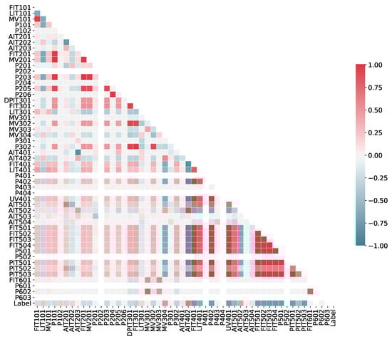
Figure 5.
Correlation between features in the SWaT dataset. A value of one represents a highly correlated feature, whereas a value of -1 represents a highly inverse correlation. Blank spaces in some features represent that the Pearson correlation could not be calculated, due to the fact that the value of that feature remained constant over the whole dataset.
Following the second task, we carried out a variance study, which showed that, in general, the features with a lower variance corresponded with those that only had a few possible values (i.e., the categorical features, such as those of motorized valve and pumps). In the top chart of Figure 6, the features with the lowest variances can be seen. We removed those features whose variance was equal to zero.
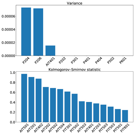
Figure 6.
Top: Features with the lowest variances. Bottom: Features with a K-S statistic score higher than 0.25.
Following the third task, we used the K-S test to check whether continuous features from both the training and the test datasets came from the same statistical distribution. As shown in the bottom chart of Figure 6, features from the sensors of chemical processes returned a higher K-S statistic. In this step, we removed the features with a K-S statistic score higher than 0.25. Additionally, we also removed the P201 feature, as we found that its behavior differed significantly between the training and test datasets, as shown in Figure 4.
A summary of the removed features and the reasons for our decisions is shown in Table 3.
Table 3.
Features removed in feature filtering.
4.4. Feature Extraction
In order to extract higher order features from the original features, we first applied autocorrelation and DFT using a 120 s window and, then, computed five statistical measures (mean, standard deviation, minimum, maximum, and range) for each operation. These new features were added to the dataset, resulting in a total of 704 features: 54 features from the original dataset and 650 new autocorrelation/DFT features. As the new extracted features had different ranges, we computed the mean and the standard deviation of the new features from the training dataset and applied standard scaling to the training and test datasets.
4.5. Anomaly Detection Method
Our first decision to build the most appropriate model was to use an LSTM neural network, as they are capable of capturing temporal patterns and predicting future states based on the previous and current state. Next, we decided to select 120 s as the length of the window n, as this provided sufficient information about the recent past of the different sensors and actuators. Furthermore, we set a value greater than one as the prediction horizon h, as neural networks tend to reproduce the last value when the prediction horizon is close to the input. Then, we set h to 10 s, and finally, we assigned the number of time steps to predict in the future, m, as 1 s, as we were interested in predicting only the next value; based on this, we computed the residual error in order to determine whether to trigger an alarm or not.
Regarding the LSTM model, we selected a set of hyperparameters, together with their respective ranges of values, to be fine-tuned during the training process. Following our methodology, hyperparameter fine-tuning was carried out by means of a grid search over the possible values. The list of hyperparameters, with their optimal values highlighted in bold, is given in Table 4.
Table 4.
Set of hyperparameters tested. The optimal ones in are listed in bold.
As a final step, we used Equation (4) to compute the z-score over the validation dataset and calculate the threshold for the maximum z-score achieved. This threshold was used to detect anomalies; that is, when the z-score computed over the test dataset was higher than the threshold.
4.6. Validation
To train and evaluate the models previously presented, we used a workstation with 32GB of RAM, an Intel i7-5930K, and an NVIDIA GeForce GTX 1080 graphic card with 8GB of video memory. The operating system running on top of the workstation was Linux, and the software used to train and evaluate the models was TensorFlow 1.12.0 [45] and Keras 2.2.4 [46].
As recommended by the first task of the validation methodology step, we used precision, recall, and F1-score to measure the performance, as SWaT is an imbalanced dataset. Our experimental results achieved values of 0.984, 0.750, and 0.851, respectively, for these performance metrics. As shown in Table 5, our solution reached the best result, in terms of precision, the DNN presented in [28] obtaining the second-best result with a precision of 0.982. Furthermore, our recall was above the average of those given in other works. In particular, the author of [26] gave a recall of 0.954, ref. [22] a recall of 0.791, ref. [29] a recall of 0.827, and [33] a recall of 0.835, these being the only works that outperformed our results. Finally, our F1-score was, again, above the average, where [22] gave an F1-score of 0.871, ref. [29] gave an F1-score of 0.873, and [33] gave an F1-score of 0.882, these being the only works that surpassed our solution.
Table 5.
Result comparison of different works using the SWaT dataset.
In addition to precision, recall, and F1-score, Table 6 shows the numbers of TP, FN, FP, and TN obtained during the validation phase using the test dataset. Our MADICS implementation achieved a high TP (43 807) and a low number of FP (701), the preferred combination in an ICS scenario. Besides, the number FP obtained by using the training dataset is zero since we are considering a threshold computed from the training/validation dataset. That threshold is selected as the maximum value obtained during the training phase.
Table 6.
False positives, false negatives, true positives, and true negatives obtained for the validation step.
The recall values achieved by different works under each cyber attack are shown in Table 7. Our approach obtained the best recall for Cyber Attack 27; whereas, for Cyber Attacks 2, 10, 11, 22, 26, 30, and 40, it achieved state-of-the-art performance. Regarding Cyber Attacks 7, 8, 17, 23, 28, 36, 37, 39, and 41, our performance was, at most, 10% lower than the performance of the rest of the works.
Table 7.
Recall comparison between different approaches on the SWaT dataset.
However, some considerations are necessary, regarding the data shown in Table 7, as follows:
- As the SWaT authors stated, some cyber attacks had no expected effect on the physical behavior of the system. In particular, Cyber Attacks 5, 9, 12, 15, and 18 had no effect; hence, they are not shown in Table 7.
- Cyber Attacks 6, 19, 20, and 38 were directed at unused chemical sensors. These attacks should have affected other sensors, but as stated by the SWaT authors, different failures prevented this, hindering the detection of these cyber attacks and causing our approach to achieve a low recall on them.
- The goal of Cyber Attack 4 was to open the motorized valve 504, but it had no impact, due to a failure. Therefore, the result by the OCSVMapproach (recall of 0.04) was considered invalid.
- Regarding Cyber Attack 13, its goal was to close the motorized valve 304; however, the cyber attack failed, and it was closed 30 min after; this is why no work was able to detect this cyber attack.
- Cyber Attack 14 was another cyber attack that had an undesirable effect: its goal was not to open the motorized valve 303. However, the cyber attack failed because the startup sequence was not carried out because the tank 301 was already full. Again, as this cyber attack had no physical effect, the 0.06 recall shown by [33] was invalid.
- Cyber Attack 29 also had no physical impact. Its goal was to turn on the pumps 201, 203, and 205. However, the SWaT dataset authors stated that the cyber attack failed because the pumps did not open, due to mechanical interlock. For this reason, the recalls shown in [28,33] were also invalid.
Taking into account the above considerations, our solution was able to detect 23 of 28 cyber attacks.
5. Discussion
MADICS establishes a clear five-step methodology for guiding the future work of cybersecurity researchers to detect cyber attacks under ICS scenarios. Despite MADICS being a general methodology to detect anomalies in ICS, we applied it to a specific industrial dataset collected from the SWaT testbed, a fully operational scaled-down water treatment plant. The results of the experiments carried out demonstrated that MADICS can help to detect cyber attacks in ICS and, therefore, can prevent the monetary losses and physical damages caused by ICS attacks. Thus, MADICS fills a gap in the literature regarding methodologies to detect cyber attacks in ICS. As Section 2 described, many works using ML and DL techniques have been proposed, but each one has followed its own steps without a common criterion or guidance, which ultimately, can lead to applying the wrong steps or making mistakes during the process. To the best of our knowledge, there are only two proposed methodologies [39,40] aimed at cyber attack detection in ICS. The main drawbacks of these methodologies are that they have rather limited cyber attack detection capacity, as they are based on classic methods (i.e., computing the mean and standard deviation to trigger an alarm) and do not consider the improvement in performance that ML and DL methods can provide.
Although the five steps of MADICS methodology are present in a typical ML/DL project, we adapted each step for use in ICS scenarios. In our first step, dataset pre-processing is performed, consisting of preparing the data to be suitable for ML/DL models. In this step, we recommend splitting the dataset and treating corrupt and missing values in a particular fashion to avoid removing useful information in an ICS scenario. In our second step, feature filtering is carried out, where we propose three different techniques to filter those features that do not provide information to the model (e.g., features that do not change their value over the entire dataset or features whose statistical distribution is not preserved between the training and test datasets). In our third step, as an ICS typically performs repetitive actions, we suggest extracting higher order features by exploiting this characteristic. This is carried out in the feature extraction step, where we recommend using the autocorrelation and Fourier transform methods. In the fourth step, as the ICS sensor and actuator data are usually available as a set of values over time, in the anomaly detection step, we suggest using a model based on LSTM, which is a neural network that is suitable to treat sequence data. Finally, in the validation step, we propose using specific metrics that are suitable for anomaly detection, in order to compare our results with those of other works.
Another relevant aspect of MADICS is that it uses semi-supervised ML and DL anomaly detection algorithms. This allows the detection models to learn the normal behavior of the ICS and trigger an anomaly alarm when a deviation from the learned behavior is observed. Additionally, we highlight the importance of both pre-processing and feature filtering steps to build an effective dataset for ICS scenarios. As shown in Section 4.2 and Section 4.3, exploring and understanding the data are critical to create practical ML and DL models. In our experimentation, dataset pre-processing allowed us to skip the first 100,000 s of the SWaT dataset corresponding to the warm-up process. Similarly, the feature filtering process allowed us to discard useless constant features and others with anomalous behavior.
In fact, comparing our work with other anomaly detection works that used the dataset collected from the SWaT testbed, we noticed that the majority of them made errors in their methodological design. The most common error is not properly studying the features to detect the warm-up process. In particular, the authors of [23,25,28,29,33] did not mention anything related to the warm-up process. Although [22,26] did propose trimming the initial records, they removed the warm-up data only partially. In [22], the authors proposed removing 16,000 samples, and [26] removed 21,600 samples. However, in our work, we showed that around 100,000 samples need to be removed. Another error, as found in [28], is normalizing the test dataset using the mean and standard deviation. The authors stated that they achieved an F1-score of 80% when normalizing the data in this way. However, when they normalized the test dataset using the mean and standard deviation from the training dataset, which is the proper way of normalizing the test dataset, they achieved an F1-score between 20 and 30%. Similarly, the authors of [33] claimed that the statistical distribution of the data in the file containing the normal behavior differed substantially from the distribution of the data in the file containing both normal and abnormal behavior. Therefore, they used the combined normal samples from both files to train the model. This is another methodological error, as the normal behavior of the test dataset must not be seen in the training phase.
Although the examined works follow a similar methodology to MADICS, their authors did not consider some steps or did not try to exploit the ICS nature, e.g., the repetitive nature of ICSs. The lack of some steps and the usage of non-optimal techniques, together with the previous methodological errors, indicate that the results presented in those works were distorted, improving the results in the majority of the cases. Besides, these methodological errors point to the urgent need for a common methodology focused on ICS scenarios. We highlight that the implementation of MADICS we carried out in this work achieved the best precision (0.984) and one of the best F1-scores (0.851), avoiding the methodological errors committed in the previous literature.
The main limitation of MADICS is that it requires the availability of a semi-supervised ready dataset; that is, the dataset must be collected during two different periods: a first period, in which the ICS is working under normal conditions, and a second period, where the ICS is suffering cyber attacks. Although the majority of related works have used semi-supervised methods, other approaches (i.e., supervised or unsupervised) can be used.
6. Conclusions
Despite the importance of detecting cyber attacks in ICS scenarios, there exists a gap in the literature regarding methodologies to follow in order to detect cyber attacks. The lack of such methodologies prevents researchers from being able to accurately compare results. In this work, we present MADICS, a methodology to detect cyber attacks in ICS scenarios based on both semi-supervised ML and DL algorithms and the anomaly detection paradigm. This methodology includes five steps: dataset pre-processing; feature filtering; feature extraction, selection, and fine-tuning; training of the anomaly detection method; and model validation. Validation of the methodology was performed using the SWaT dataset. This dataset was captured from a fully operational scaled-down water treatment plant during 11 days of continuous operation: seven days under normal operation and four days under cyber attacks. In the experiment carried out to test our methodology, the resulting model achieved a state-of-the-art precision score (0.984), whereas both the recall (0.750) and F1-score (0.851) values were above the average of those in relevant works in the literature. Concerning the detection performance for each cyber attack, our model trained following MADICS was able to detect 23 cyber attacks of 28. As future work and to improve confidence in the results, we intend to perform additional experiments with other industrial datasets. Another future direction is to study how to improve the detection performance on cyber attacks with an extremely low recall rate.
Author Contributions
Conceptualization, Á.L.P.G.; data curation, Á.L.P.G. and A.H.C.; formal analysis, Á.L.P.G. and L.F.M.; funding acquisition, F.J.G.C.; investigation, Á.L.P.G., L.F.M., A.H.C., and F.J.G.C.; methodology, Á.L.P.G., L.F.M., and A.H.C.; project administration, F.J.G.C.; software, Á.L.P.G. and L.F.M.; supervision, F.J.G.C.; validation, L.F.M. and F.J.G.C.; writing, original draft, Á.L.P.G. and L.F.M.; writing, review and editing, A.H.C. and F.J.G.C. All authors have read and agreed to the published version of the manuscript.
Funding
This work was funded by Spanish Ministry of Science, Innovation and Universities, FEDER funds, under Grant RTI2018-095855-B-I00, and the Government of Ireland, through the IRC post-doc fellowship (Grant Code GOIPD/2018/466).
Conflicts of Interest
The authors declare no conflict of interest.
References
- Jiang, B.; Yang, J.; Ding, G.; Wang, H. Cyber-physical security design in multimedia data cache resource allocation for industrial networks. IEEE Trans. Ind. Inform. 2019, 15, 6472–6480. [Google Scholar] [CrossRef]
- Miller, B.; Rowe, D. A survey SCADA of and critical infrastructure incidents. In Proceedings of the 1st Annual Conference on Research in Information Technology, Calgary, AB, Canada, 11–13 October 2012; pp. 51–56. [Google Scholar]
- Nicholson, A.; Webber, S.; Dyer, S.; Patel, T.; Janicke, H. SCADA security in the light of Cyber-Warfare. Comput. Secur. 2012, 31, 418–436. [Google Scholar] [CrossRef]
- Hemsley, K.E.; Fisher, E.; Ronald, D. History of Industrial Control System Cyber Incidents; Technical Report; Idaho National Lab. (INL): Idaho Falls, ID, USA, 2018.
- Karnouskos, S. Stuxnet worm impact on industrial cyber-physical system security. In Proceedings of the IECON 2011 37th Annual Conference of the IEEE Industrial Electronics Society, Melbourne, Australia, 7–10 November 2011; pp. 4490–4494. [Google Scholar]
- Kumar, M. Irongate new stuxnet-like malware targets industrial control systems. The Hacker News, 2016. [Google Scholar]
- Fan, X.; Fan, K.; Wang, Y.; Zhou, R. Overview of cyber-security of industrial control system. In Proceedings of the 2015 International Conference on Cyber Security of Smart Cities, Industrial Control System and Communications (SSIC), Shanghai, China, 5–7 August 2015; pp. 1–7. [Google Scholar]
- Jie, P.; Li, L. Industrial Control System Security. In Proceedings of the 2011 Third International Conference on Intelligent Human-Machine Systems and Cybernetics, Hangzhou, China, 26–27 August 2011; Volume 2, pp. 156–158. [Google Scholar]
- Pillitteri, V.Y.; Brewer, T.L. Guidelines for Smart Grid Cybersecurity; Technical Report; NIST Interagency/Internal Report (NISTIR): Gaithersburg, MD, USA, 2014.
- Van, N.T.; Thinh, T.N.; Sach, L.T. An anomaly-based network intrusion detection system using Deep learning. In Proceedings of the 2017 International Conference on System Science and Engineering (ICSSE), Ho Chi Minh City, Vietnam, 21–23 July 2017; pp. 210–214. [Google Scholar]
- Zitta, T.; Neruda, M.; Vojtech, L.; Matejkova, M.; Jehlicka, M.; Hach, L.; Moravec, J. Penetration Testing of Intrusion Detection and Prevention System in Low-Performance Embedded IoT Device. In Proceedings of the 2018 18th International Conference on Mechatronics-Mechatronika (ME), Brno, Czech Republic, 5–7 December 2018; pp. 1–5. [Google Scholar]
- Fernández Maimó, L.; Perales Gómez, A.L.; García Clemente, F.J.; Gil Pérez, M.; Martínez Pérez, G. A Self-Adaptive Deep Learning-Based System for Anomaly Detection in 5G Networks. IEEE Access 2018, 6, 7700–7712. [Google Scholar] [CrossRef]
- Fernández Maimó, L.; Huertas Celdrán, A.; Gil Pérez, M.; García Clemente, F.J.; Martínez Pérez, G. Dynamic management of a deep learning-based anomaly detection system for 5G networks. J. Ambient Intell. Humaniz. Comput. 2019, 10, 3083–3097. [Google Scholar] [CrossRef]
- Fernández Maimó, L.; Huertas Celdrán, A.; Perales Gómez, A.L.; García Clemente, F.J.; Weimer, J.; Lee, I. Intelligent and dynamic ransomware spread detection and mitigation in integrated clinical environments. Sensors 2019, 19, 1114. [Google Scholar] [CrossRef] [PubMed]
- Goh, J.; Adepu, S.; Junejo, K.N.; Mathur, A. A Dataset to Support Research in the Design of Secure Water Treatment Systems. In Critical Information Infrastructures Security; Havarneanu, G., Setola, R., Nassopoulos, H., Wolthusen, S., Eds.; Springer International Publishing: Cham, Switzerland, 2017; pp. 88–99. [Google Scholar]
- Vávra, J.; Hromada, M. Comparison of the Intrusion Detection System Rules in Relation with the SCADA Systems. In Software Engineering Perspectives and Application in Intelligent Systems; Silhavy, R., Senkerik, R., Oplatkova, Z.K., Silhavy, P., Prokopova, Z., Eds.; Springer International Publishing: Cham, Switzerland, 2016; pp. 159–169. [Google Scholar]
- Yang, Y.; McLaughlin, K.; Littler, T.; Sezer, S.; Wang, H. Rule-based intrusion detection system for SCADA networks. IET Conf. Proc. 2013, 1–4. [Google Scholar] [CrossRef]
- Mitchell, R.; Chen, I. Behavior-Rule Based Intrusion Detection Systems for Safety Critical Smart Grid Applications. IEEE Trans. Smart Grid 2013, 4, 1254–1263. [Google Scholar] [CrossRef]
- Kleinmann, A.; Wool, A. A Statechart-Based Anomaly Detection Model for Multi-Threaded SCADA Systems. In Critical Information Infrastructures Security; Rome, E., Theocharidou, M., Wolthusen, S., Eds.; Springer International Publishing: Cham, Switaerland, 2016; pp. 132–144. [Google Scholar]
- Petrillo, A.; Picariello, A.; Santini, S.; Scarciello, B.; Sperlí, G. Model-based vehicular prognostics framework using Big Data architecture. Comput. Ind. 2020, 115, 103177. [Google Scholar] [CrossRef]
- Men, J.; Lv, Z.; Zhou, X.; Han, Z.; Xian, H.; Song, Y. Machine Learning Methods for Industrial Protocol Security Analysis: Issues, Taxonomy, and Directions. IEEE Access 2020, 8, 83842–83857. [Google Scholar] [CrossRef]
- Kravchik, M.; Shabtai, A. Detecting Cyber Attacks in Industrial Control Systems Using Convolutional Neural Networks. In Proceedings of the 2018 Workshop on Cyber-Physical Systems Security and PrivaCy; Association for Computing Machinery: New York, NY, USA, 2018; pp. 72–83. [Google Scholar]
- Shalyga, D.; Filonov, P.; Lavrentyev, A. Anomaly detection for water treatment system based on neural network with automatic architecture optimization. arXiv 2018, arXiv:1807.07282. [Google Scholar]
- Lavin, A.; Ahmad, S. Evaluating Real-Time Anomaly Detection Algorithms—The Numenta Anomaly Benchmark. In Proceedings of the 2015 IEEE 14th International Conference on Machine Learning and Applications (ICMLA), Miami, FL, USA, 9–11 December 2015; pp. 38–44. [Google Scholar]
- Zizzo, G.; Hankin, C.; Maffeis, S.; Jones, K. Intrusion Detection for Industrial Control Systems: Evaluation Analysis and Adversarial Attacks. arXiv 2019, arXiv:1911.04278. [Google Scholar]
- Li, D.; Chen, D.; Jin, B.; Shi, L.; Goh, J.; Ng, S.K. MAD-GAN: Multivariate Anomaly Detection for Time Series Data with Generative Adversarial Networks. In Artificial Neural Networks and Machine Learning—ICANN 2019: Text and Time Series; Tetko, I.V., Kůrková, V., Karpov, P., Theis, F., Eds.; Springer International Publishing: Cham, Switzerland, 2019; pp. 703–716. [Google Scholar]
- Kim, J.; Yun, J.H.; Kim, H.C. Anomaly detection for industrial control systems using sequence-to-sequence neural networks. arXiv 2019, arXiv:1911.04831. [Google Scholar]
- Inoue, J.; Yamagata, Y.; Chen, Y.; Poskitt, C.M.; Sun, J. Anomaly Detection for a Water Treatment System Using Unsupervised Machine Learning. In Proceedings of the 2017 IEEE International Conference on Data Mining Workshops (ICDMW), New Orleans, LA, USA, 18–21 November 2017; pp. 1058–1065. [Google Scholar]
- Kravchik, M.; Shabtai, A. Efficient cyber attacks detection in industrial control systems using lightweight neural networks. arXiv 2019, arXiv:1907.01216. [Google Scholar]
- Liu, L.; Hu, M.; Kang, C.; Li, X. Unsupervised Anomaly Detection for Network Data Streams in Industrial Control Systems. Information 2020, 11, 105. [Google Scholar] [CrossRef]
- Tomlin, L.; Farnam, M.R.; Pan, S. A clustering approach to industrial network intrusion detection. In Proceedings of the 2016 Information Security Research and Education (INSuRE) Conference (INSuRECon-16), University of Alabama in Huntsville, Huntsville, AL, USA, 30 September 2016. [Google Scholar]
- Schneider, P.; Böttinger, K. High-performance unsupervised anomaly detection for cyber-physical system networks. In Proceedings of the 2018 Workshop on Cyber-Physical Systems Security and PrivaCy, Toronto, ON, Canada, 19 October 2018; pp. 1–12. [Google Scholar]
- Elnour, M.; Meskin, N.; Khan, K.; Jain, R. A Dual-Isolation-Forests-Based Attack Detection Framework for Industrial Control Systems. IEEE Access 2020, 8, 36639–36651. [Google Scholar] [CrossRef]
- Khan, A.A.Z. Misuse Intrusion Detection Using Machine Learning for Gas Pipeline SCADA Networks. In Proceedings of the International Conference on Security and Management (SAM), Las Vegas, NV, USA, 29 July–1 August 2019; The Steering Committee of The World Congress in Computer Science, Computer Engineering and Applied Computing (WorldComp): San Diego, CA, USA, 2019; pp. 84–90. [Google Scholar]
- Alhaidari, F.A.; AL-Dahasi, E.M. New Approach to Determine DDoS Attack Patterns on SCADA System Using Machine Learning. In Proceedings of the 2019 International Conference on Computer and Information Sciences (ICCIS), Sakaka, Saudi Arabia, 3–4 April 2019; pp. 1–6. [Google Scholar]
- Perales Gómez, Á.L.; Fernández Maimó, L.; Huertas Celdrán, A.; García Clemente, F.J.; Cadenas Sarmiento, C.; Del Canto Masa, C.J.; Méndez Nistal, R. On the Generation of Anomaly Detection Datasets in Industrial Control Systems. IEEE Access 2019, 7, 177460–177473. [Google Scholar] [CrossRef]
- Trilles, S.; Belmonte, O.; Schade, S.; Huerta, J. A domain-independent methodology to analyze IoT data streams in real-time. A proof of concept implementation for anomaly detection from environmental data. Int. J. Digit. Earth 2017, 10, 103–120. [Google Scholar] [CrossRef]
- Salazar, F.; Toledo, M.Á.; González, J.M.; Oñate, E. Early detection of anomalies in dam performance: A methodology based on boosted regression trees. Struct. Control Health Monit. 2017, 24, e2012. [Google Scholar] [CrossRef]
- Pinelli, M.; Venturini, M.; Burgio, M. Statistical methodologies for reliability assessment of gas turbine measurements. In ASME Turbo Expo 2003, Collocated with the 2003 International Joint Power Generation Conference; American Society of Mechanical Engineers Digital Collection: New York, NY, USA, 2003; pp. 787–793. [Google Scholar]
- Fabio Ceschini, G.; Gatta, N.; Venturini, M.; Hubauer, T.; Murarasu, A. Optimization of Statistical Methodologies for Anomaly Detection in Gas Turbine Dynamic Time Series. J. Eng. Gas Turbines Power 2017, 140. [Google Scholar] [CrossRef]
- Sarkar, B.K. A case study on partitioning data for classification. Int. J. Inf. Decis. Sci. 2016, 8, 73–91. [Google Scholar] [CrossRef]
- Russac, Y.; Caelen, O.; He-Guelton, L. Embeddings of categorical variables for sequential data in fraud context. In International Conference on Advanced Machine Learning Technologies and Applications; Springer: Cham, Switzerland, 2018; pp. 542–552. [Google Scholar]
- Hunter, J.D. Matplotlib: A 2D graphics environment. Comput. Sci. Eng. 2007, 9, 90–95. [Google Scholar] [CrossRef]
- Waskom, M.; Botvinnik, O.; Ostblom, J.; Lukauskas, S.; Hobson, P.; Gelbart, M.; Gemperline, D.C.; Augspurger, T.; Halchenko, Y.; Cole, J.B.; et al. mwaskom/seaborn: V0.8.1 (September 2017). Available online: https://github.com/mwaskom/seaborn (accessed on 15 September 2020).
- Abadi, M.; Agarwal, A.; Barham, P.; Brevdo, E.; Chen, Z.; Citro, C.; Corrado, G.S.; Davis, A.; Dean, J.; Devin, M.; et al. Tensorflow: Large-scale machine learning on heterogeneous distributed systems. arXiv 2016, arXiv:1603.04467. [Google Scholar]
- Chollet, F. Keras. 2015. Available online: https://keras.io (accessed on 15 September 2020).


© 2020 by the authors. Licensee MDPI, Basel, Switzerland. This article is an open access article distributed under the terms and conditions of the Creative Commons Attribution (CC BY) license (http://creativecommons.org/licenses/by/4.0/).